Variable Control Charts – Linear Failure Rate Distribution
M. Ch. Priya
Department of Mathematics, Jazan University Jazan, Kingdom of Saudi Arabia
R. R. L. Kantam
Department of Statistics, Acharya Nagarjuna University Andhra Pradesh, India
Abstract
The well-known Linear Failure Rate Distribution (LFRD) is considered. A process variate following LFRD is proposed in order to develop control charts for subgroup mean and subgroup range. In view of the limitations on LFRD the theoretical control limits are obtained through some approximations and the resulting control chart limits are worked out. Comparison with the control limits of similar variable control charts is also presented.
Keywords: Linear failure rate distribution, Control charts, Sub group mean and range.
1. Introduction
It is well-known that a control chart is a graphical device that detects variations in any variable quality characteristic of a product. Given a specified target value of the quality characteristic say 0 , production of the concerned product has to be so designed that the
associated quality characteristic for the products should be ideally equal to 0 , if not ,
very close to 0 on its either side. That is, if the products are showing variations in the
desirable quality, the variations must be within control in some admissible sense. That is, there should be two limits within which the allowable variations are supposed to fall. Whenever this happens, the production process is defined to be in control. Otherwise, it is out of control. Based on this principle it is necessary to think of the control limits on either side of the target value in such a way that under normal conditions the limits should include most of the observations. With this backdrop the well-known Shewhart control charts are developed under the assumption that the quality characteristic follows a normal distribution.
If 𝑥1, 𝑥2, . . 𝑥𝑛 is a collection of observations of size ‘n’ on a variable quality characteristic of a product, tn is a statistic based on this sample, the control limits of Shewhart variable
control chart are 𝐸(𝑡𝑛) ± 3𝑆. 𝐸. (𝑡𝑛). Under repeated sampling of size ‘n’ at each time (say k times) the graph of the points (i, tn(i)), i=1 to k, where tn(i) is the value of tn based
on n observations of the ith sample, along with three lines parallel to horizontal axis at
𝐸(𝑡𝑛) − 3 𝑆. 𝐸. (𝑡𝑛), 𝐸(𝑡𝑛) and 𝐸(𝑡𝑛) + 3 𝑆. 𝐸. (𝑡𝑛) is called control chart for the statistic tn. For instance, if tn is 𝑋̅, the graph is control chart for mean, if tn is range the
the distribution of tn may not be normal. Even if asymptotic normality of tn is made use
of, it is valid only in large samples. However, in quality control studies data is always in small samples only. Therefore if the population is not normal there is a need to develop a separate procedure for the construction of control limits.
Skewed distributions to develop control charts are considered by many authors. Edgemen (1989), Kantam and Sriram (2001), Kantam et al. (2006), Kantam and Priya (2010), Kantam and Srinivasa Rao (2010), Kantam and Priya (2011), Srinivasa Rao and Kantam (2012) and the references therein are a few contributions in this direction. Besides these works, many researchers have been working on the theory of control charts for skewed as well as symmetrically distributed data that include. Amin and Miller (1993), Costa (1995), Costa (1996), Amin and Widmaier (1999) , Wu et al. (2002), Kan and Yazici (2006), Gob et al. (2006), Mahadik and Shirke (2007), Zhang et al. (2011), Derya and Canan (2012). In this paper we consider the well-known linear failure rate distribution (LFRD) - a skewed distribution and attempt to develop control limits for a variable quality characteristic assumed to follow LFRD.
The density function, cumulative distribution function, hazard or failure rate function of LFRD are
𝑓(𝑥) = (𝑎 + 𝑏𝑥)𝑒−(𝑎𝑥+𝑏𝑥22 ); 𝑥 > 0, 𝑎 > 0, 𝑏 > 0, (1.1)
𝐹(𝑥) = 1 − 𝑒−(𝑎𝑥+𝑏𝑥22 ); 𝑥 > 0, 𝑎 > 0, 𝑏 > 0, (1.2)
ℎ(𝑥) = 𝑎 + 𝑏𝑥. (1.3)
Ananda Sen (2005) gave a detailed review along with the distributional characteristics and inferential aspects of LFRD. Some basic features of LFRD are as follows:
Mean:
𝜇 = √2𝜋𝑏 𝑒𝑎2⁄2𝑏
(1 − Ф(𝑎 √𝑏⁄ )), (1.4)
where Ф(. ) denotes the cumulative distribution function of a standard normal variate. Variance:
𝜎2 =2
𝑏(1 − 𝑎𝜇) − 𝜇
2, (1.5)
Mode:
𝑀 = (√1𝑏−𝑎𝑏) 𝐼(𝑎2< 𝑏), (1.6)
where I(.) denotes indicator function. 100 pth Percentile:
𝐹−1(𝑝) = √(𝑎 𝑏)
2
−2log (1−𝑝)𝑏 −𝑎𝑏, (1.7)
and hence median is
𝑀𝑑 = √(𝑎) 2
The sampling distribution of mean and range of a random sample of size ‘n’ drawn from LFRD are not in analytical form thereby resulting in lack of exact percentiles of these sampling distributions analytically. Hence we have to try for approximate control limits/ corrected control limits if acceptable. We have addressed this problem in two different approaches.
(i) Fixing LFRD as a suitable model for a quality data and trying for approximate quality control constants for the data.
(ii) Approximating LFRD by a reasonable and admissible model for which exact quality control constants are available and making use of them for LFRD data. For approach (i) we borrowed the results of Chan and Cui (2003). For approach (ii) we made use of the results in Kantam and Sriram (2001). The rest of the paper is organized as follows. The summary of Chan and Cui (2003) and its adoption to LFRD are given in Section 2. The content of Kantam and Sriram (2001) and its adoption to LFRD, the performance of the LFRD based control charts by the above two approaches are given in Section 3, followed by an example in Section 4.
2. LFRD Based Control Charts: Approach-I
(a) Principle of Skewness Corrected Control Chart (Chan and Cui, 2003)
Let X be a standardized random variable with mean 0, standard deviation 1, coefficient of skewness k3. Let 𝑥1, 𝑥2, . . 𝑥𝑛 be a sample from the distribution of a process variate with mean µ and standard deviation σ. We know that when the process parameters are unknown the Shewhart limits are given by
Shewhart𝑋̅ Chart:
𝑈𝐶𝐿𝑋̅ = 𝑋̿ + 𝐴2𝑅̅, 𝐶𝐿𝑋̅ = 𝑋̿, 𝐿𝐶𝐿𝑋̅ = 𝑋̿ − 𝐴2𝑅̅,
Shewhart R Chart:
𝑈𝐶𝐿𝑅 = 𝐷4𝑅̅, 𝐶𝐿𝑅 = 𝑅̅, 𝐿𝐶𝐿𝑅 = 𝐷3𝑅̅.
where the constants A2, D3, D4 are available for specified sub group sizes from any
standard text book on statistical quality control.
The control limits and the central line for a skewness corrected (SC) control chart for 𝑋̅ chart are
𝑆𝐶 𝑋̅ 𝐶ℎ𝑎𝑟𝑡:
{
𝑈𝐶𝐿𝑋̅= 𝑋̿ + (3 +4𝑘1+0.2𝑘3⁄(3√𝑛) 32⁄𝑛)
𝑅̅
𝑑2∗√𝑛≡ 𝑋̿ + 𝐴𝑈 ∗𝑅̅,
𝐶𝐿𝑋̅ = 𝑋̿, 𝐿𝐶𝐿𝑋̅= 𝑋̿ + (−3 +4𝑘3⁄(3√𝑛)
1+0.2𝑘32⁄𝑛) 𝑅̅
𝑑2∗√𝑛≡ 𝑋̿ − 𝐴𝐿 ∗𝑅.̅
(2.1)
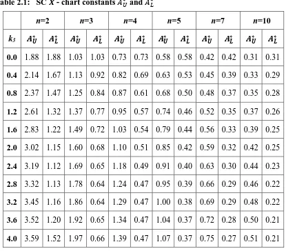
Table 2.1: SC 𝑿̅ - chart constants 𝐴𝑈∗ and 𝐴 𝐿 ∗
n=2 n=3 n=4 n=5 n=7 n=10
k3 𝑨𝑼∗ 𝑨𝑳∗ 𝑨𝑼∗ 𝑨𝑳∗ 𝑨𝑼∗ 𝑨∗𝑳 𝑨𝑼∗ 𝑨𝑳∗ 𝑨∗𝑼 𝑨𝑳∗ 𝑨𝑼∗ 𝑨𝑳∗
0.0 1.88 1.88 1.03 1.03 0.73 0.73 0.58 0.58 0.42 0.42 0.31 0.31
0.4 2.14 1.67 1.13 0.92 0.82 0.69 0.63 0.53 0.45 0.39 0.33 0.29
0.8 2.37 1.47 1.25 0.84 0.87 0.61 0.68 0.50 0.48 0.37 0.35 0.28
1.2 2.61 1.32 1.37 0.77 0.95 0.57 0.74 0.46 0.52 0.35 0.37 0.26
1.6 2.83 1.22 1.49 0.72 1.03 0.54 0.79 0.44 0.56 0.33 0.39 0.25
2.0 3.02 1.15 1.60 0.68 1.10 0.51 0.85 0.42 0.59 0.32 0.42 0.25
2.4 3.19 1.12 1.69 0.65 1.18 0.49 0.91 0.40 0.63 0.30 0.44 0.23
2.8 3.32 1.13 1.78 0.64 1.24 0.47 0.95 0.39 0.66 0.29 0.46 0.22
3.2 3.45 1.16 1.86 0.64 1.29 0.47 1.00 0.38 0.69 0.29 0.48 0.22
3.6 3.52 1.20 1.92 0.65 1.34 0.47 1.04 0.37 0.72 0.28 0.50 0.21
4.0 3.59 1.52 1.97 0.66 1.39 0.47 1.07 0.37 0.75 0.27 0.51 0.21
If the value of k3 for our specified model is not one of those in the above table it is
suggested to take the nearest tabulated value of k3 or to use interpolation.
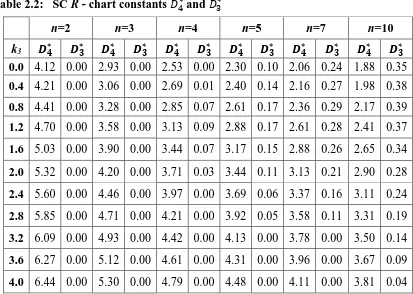
Proceeding on similar lines the control limits for the skewness corrected range chart are given by
𝑆𝐶 𝑅̅ 𝐶ℎ𝑎𝑟𝑡:
{
𝑈𝐶𝐿𝑅 = [1 + (3 + 𝑑4∗)𝑑3 ∗
𝑑2∗] 𝑅̅ ≡ 𝐷4 ∗𝑅̅,
𝐶𝐿𝑋̅ = 𝑅̅,
𝐿𝐶𝐿𝑋̅ = [1 + (−3 + 𝑑4∗)𝑑3∗ 𝑑2∗]
+
𝑅̅ ≡ 𝐷3∗𝑅̅ .
(2.2)
Table 2.2: SC R - chart constants 𝐷4∗and 𝐷 3∗
n=2 n=3 n=4 n=5 n=7 n=10
k3 𝑫𝟒∗ 𝑫𝟑∗ 𝑫𝟒∗ 𝑫𝟑∗ 𝑫𝟒∗ 𝑫∗𝟑 𝑫𝟒∗ 𝑫𝟑∗ 𝑫∗𝟒 𝑫𝟑∗ 𝑫𝟒∗ 𝑫𝟑∗
0.0 4.12 0.00 2.93 0.00 2.53 0.00 2.30 0.10 2.06 0.24 1.88 0.35
0.4 4.21 0.00 3.06 0.00 2.69 0.01 2.40 0.14 2.16 0.27 1.98 0.38
0.8 4.41 0.00 3.28 0.00 2.85 0.07 2.61 0.17 2.36 0.29 2.17 0.39
1.2 4.70 0.00 3.58 0.00 3.13 0.09 2.88 0.17 2.61 0.28 2.41 0.37
1.6 5.03 0.00 3.90 0.00 3.44 0.07 3.17 0.15 2.88 0.26 2.65 0.34
2.0 5.32 0.00 4.20 0.00 3.71 0.03 3.44 0.11 3.13 0.21 2.90 0.28
2.4 5.60 0.00 4.46 0.00 3.97 0.00 3.69 0.06 3.37 0.16 3.11 0.24
2.8 5.85 0.00 4.71 0.00 4.21 0.00 3.92 0.05 3.58 0.11 3.31 0.19
3.2 6.09 0.00 4.93 0.00 4.42 0.00 4.13 0.00 3.78 0.00 3.50 0.14
3.6 6.27 0.00 5.12 0.00 4.61 0.00 4.31 0.00 3.96 0.00 3.67 0.09
4.0 6.44 0.00 5.30 0.00 4.79 0.00 4.48 0.00 4.11 0.00 3.81 0.04
If the distribution under consideration is a skewed one, its coefficient of skewness say k3
is first evaluated by any standard formula. Particular to the subgroup size where a control chart for mean is needed, we identify the control limits 𝐴∗𝐿, 𝐴∗𝑈 from the bivariate Table 2.1 with the help of linear interpolation if necessary. The pair (𝐴𝐿∗, 𝐴𝑈∗) so selected when used in the formula (2.1) would give the control limits of the mean chart based on SC method.
(b) Adoption of Chan and Cui (2003) to Control Charts Based on LFRD Variate
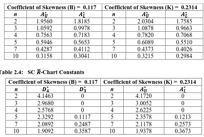
We know that the LFRD is a skewed distribution. Here we chose the Bowley’s, Kelly’s formulae for finding coefficient of skewness which are respectively given by
𝑘3(𝐵) =𝑄3−2𝑄2+𝑄1
𝑄3−𝑄1 , 𝑘3(𝐾)=
𝑃90−2𝑃50+𝑃10
𝑃90−𝑃10 , where 𝑄𝑖(i=1, 2, 3) is the i
th quartile and 𝑃
𝑖 (i= 10, 50, 90) is the percentile of the LFRD.
We fix the LFRD parameters for developing control chart constants as a=3, b=25. The Bowley’s and Kelly’s coefficients of skewness for LFRD are 0.117 and 0.2314 respectively. It can be seen from Table 2.1, that the values of our coefficients of skewness are not figured in Table 2.1. Accordingly, as per the suggestion in Chan and Cui (2003) we have resorted to interpolation in order to get the values of 𝐴𝐿∗, 𝐴𝑈∗, 𝐷3∗, 𝐷4∗ corresponding to the k3 values under discussion.
As a result of our interpolation technique the following are the values of 𝐴𝐿∗ ,𝐴𝑈∗ and 𝐷3∗ ,
𝐷4∗ corresponding to specified choices of n and k
3. These are given in the following
Table 2.3: SC 𝑿̅-Chart Constants
Coefficient of Skewness (B) = 0.117 Coefficient of Skewness (K) = 0.2314
n 𝑨𝑼∗ 𝑨𝑳∗ n 𝑨𝑼∗ 𝑨𝑳∗
2 1.9560 1.8185 2 2.0304 1.7585
3 1.0592 0.9978 3 1.0878 0.9663
4 0.7563 0.7183 4 0.7820 0.7068
5 0.5946 0.5653 5 0.6089 0.5510
7 0.4287 0.4112 7 0.4373 0.4026
10 0.3158 0.3041 10 0.3215 0.2984
Table 2.4: SC 𝑹̅-Chart Constants
Coefficient of Skewness (B) = 0.117 Coefficient of Skewness (K) = 0.2314
n 𝑫𝟒∗ 𝑫𝟑∗ n 𝑨𝑼∗ 𝑨𝑳∗
2 4.1463 0 2 4.1720 0
3 2.9680 0 3 3.0052 0
4 2.5768 0 4 2.6225 0
5 2.3292 0.1117 5 2.3578 0.1213
7 2.0892 0.2487 7 2.1178 0.2573
10 1.9092 0.3587 10 1.9378 0.3673
3. LFRD Based Control Charts: Approach-II
(a) Exact Control Limits for Gamma Variate: Kantam and Sriram (2001)
The probability density function of the gamma distribution having shape parameter 2 and scale parameter σ is given by
𝑔(𝑥) = (𝑥 𝜎⁄ 2) exp (−𝑥 𝜎) ,⁄ 𝜎 > 0, 𝑥 > 0. (3.1)
If 𝑥1, 𝑥2, . . 𝑥𝑛 is a random sample of size n from a gamma distribution with shape parameter 2 and scale parameter σ, it is known that 𝑥̅/2 is the maximum likelihood estimator of σ. It is the UMVUE of σ as well. The sampling distribution of 𝑛𝑥̅ 𝜎⁄ is gamma with shape parameter 2n. This fact can be used to get equitailed 99.73% probability limits of 𝑥̅ analogous to the corresponding 3σ limits of an 𝑋̅chart in the case of normal distributions. Let L1 and L2 be these two equitailed 99.73% percentiles of the
gamma distribution with shape parameter 2n. Then,
𝑃 {𝐿1≤ 𝑛𝑥̅𝜎 ≤ 𝐿3} = 0.9973
𝑃 {𝑛𝑥̅𝜎 < 𝐿1} = 0.00135
𝑃 {𝑛𝑥̅𝜎 < 𝐿2} = 0.99865 }
(3.2)
L1 and L2 depend on the sample size n. Using tables of the incomplete gamma function to
find these two values for a given n, the following probability statement can be made:
That is, in repeated sampling say, (k times) of size n each time with the arithmetic mean of the ith sample as 𝑥̅𝑖, i=1,2,….,k, a plot of the serial number of the sample against its corresponding arithmetic mean, provides a graph of the control chart for averages. The unknown parameter σ is estimated by its maximum likelihood estimator, 𝑥̅ 2⁄ . Over repeated sampling (subgrouping), σ is estimated by 𝑥̿ 2⁄ , where 𝑥̿ is the grand mean of all the subgroups. Then estimated version of (3.3) becomes,
𝑃{𝑀1𝑋̿ < 𝑋̅ < 𝑀2𝑋̿} = 0.9973,
where Mi= Li/2n; i = 1, 2; which are given in Table 3.1. These can be used to get the
control chart limits.
To develop the control chart for the ranges, the percentile points of the sampling distribution of the sample range are needed. In the case of the gamma distribution, these percentile points of the sample range are not available in a published form till 2001. These are tabulated in Kantam and Sriram (2001) with the following methodology. If W is the range of a sample of size n from a continuous probability model with f(.) and F(.) as the probability density function and cumulative distribution function respectively, it is known that the cumulative distribution of W is given as:
𝐺(𝑤) = 𝑛 ∫+∞𝑓(𝑥)[𝐹(𝑥 + 𝑤) − 𝐹(𝑥)]𝑛−1𝑑𝑥.
−∞ (3.4)
Replacing f(.) and F(.) in equation (3.4) with the corresponding gamma distribution function with shape parameter 2, the following expression can be obtained:
𝐺(𝑤) = ∑ {(−1)𝑗(𝑛 − 1
𝑗 ) 𝑤𝑗𝑒−𝑗𝑤[ ∑ (−1)𝑘𝑒−𝑘𝑤(
𝑛 − 𝑗 − 1
𝑘 )
(𝑛−𝑗−1)
𝑘=0
]
𝑛−1
𝑗=0
[∑𝑛−𝑗−1𝑖=0 (𝑛−𝑗−1𝑖 )((𝑖 + 1)! 𝑛⁄ 𝑖+1)]} (3.5)
From this equation, the values of G(w) have been tabulated for n =2(1)10, w= 0.0 (0.05) 14.55.
In order to get the control limits for range chart we have to find two constants 𝑐1, 𝑐2 such that
𝑃{𝑐1 < 𝑅 < 𝑐2} = 0.9973 (3.6)
If ‘w’ is the sample range in a standard gamma (𝑤 = 𝑍(𝑛)− 𝑍(1)) we know that R= σw. Hence equation (3.6) becomes
P{ 𝒄𝟏< σ w < 𝒄𝟐}=0.9973
𝑷 {𝒄𝟏
𝝈 < 𝑤 < 𝒄𝟐
𝝈} = 𝟎. 𝟗𝟗𝟕𝟑
Let 𝒄𝟏 = 𝒘𝟎.𝟎𝟎𝟏𝟑𝟓𝝈, 𝒄𝟐= 𝒘𝟎.𝟗𝟗𝟖𝟔𝟓𝝈
i.e., 𝒄𝟏= 𝒘𝟎.𝟎𝟎𝟏𝟑𝟓𝑹 𝜶(𝒏)−𝜶(𝟏), 𝒄𝟐=
𝒘𝟎.𝟗𝟗𝟖𝟔𝟓𝑹 𝜶(𝒏)−𝜶(𝟏)
i.e., c1=M3R, c2=M4R
where 𝑴𝟑= 𝜶𝒘𝟎.𝟎𝟎𝟏𝟑𝟓
(𝒏)−𝜶(𝟏), 𝑴𝟒=
𝒘𝟎.𝟗𝟗𝟖𝟔𝟓 𝜶(𝒏)−𝜶(𝟏)
The constants M3, M4 depend only on n, the mathematical model of standard gamma
distribution and its moments of extreme sample order statistics. These can be calculated a priori outside the data set. Over repeated sub grouping R is replaced by the mean of ranges𝑅̅. Thus the control limits of range chart would be 𝑀3𝑅̅, 𝑀4𝑅̅ where M3, M4 are
given in Table 3.1.
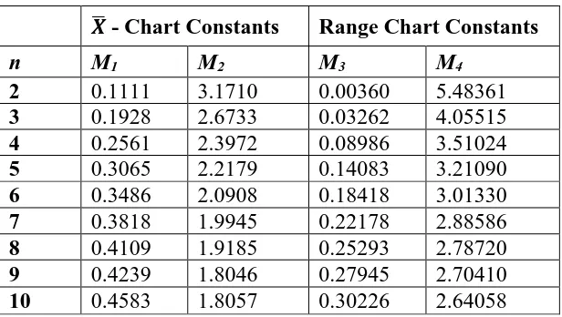
Table -3.1: Control Chart Constants
𝑿̅ - Chart Constants Range Chart Constants
n M1 M2 M3 M4
2 0.1111 3.1710 0.00360 5.48361
3 0.1928 2.6733 0.03262 4.05515
4 0.2561 2.3972 0.08986 3.51024
5 0.3065 2.2179 0.14083 3.21090
6 0.3486 2.0908 0.18418 3.01330
7 0.3818 1.9945 0.22178 2.88586
8 0.4109 1.9185 0.25293 2.78720
9 0.4239 1.8046 0.27945 2.70410
10 0.4583 1.8057 0.30226 2.64058
(b) Adoption of Kantam and Sriram (2001) to LFRD
As mentioned in Section 1, we try to mitigate the problem of non availability of exact control chart constants for LFRD by using exact control chart constants of gamma distribution with LFRD data. That is, data will be generated form LFRD and exact limits of gamma model will be used to develop control chart limits. In this direction we have attempted the following simulation methodology.
Random samples of size n= 2,3,4,5,7,10 are generated from LFRD a=3, b=25. For each sample, the mean and range are calculated, the grand mean and the mean of the ranges are also computed. Using the constants 𝐴𝐿∗ , 𝐴𝑈∗ of Table 2.3; M1, M2 of Table 3.1, the
control limits of 𝑋̅ – chart for LFRD data are calculated. The proportion of sub-group means that fall within pair of control limits out of 10000 runs is noted down. This proportion is named as coverage probability of the respective pair of control limits. Similarly using the constants 𝐷3∗ , 𝐷4∗ of Table 2.4 and the constants M3, M4 of Table 3.1
probabilities for the various pairs of control limits are presented separately for 𝑋̅ chart and Range chart in Table 3.2 and Table 3.3 respectively.
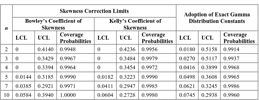
From Table 3.2 we see that 𝑋̅ chart based on skewness correction control limits using Kelly’s coefficient of skewness seems to be preferable with respect to coverage probabilities. On the other hand, Table 3.3 shows that adoption of exact control chart constants of gamma distribution for LFRD data is rated as preferable. We therefore suggest skewness corrected constants for 𝑋̅ chart and exact constants of gamma distribution for range chart of LFRD data.
Table 3.2: Control Limits for 𝑿̅ - Chart
n
Skewness Correction Limits
Adoption of Exact Gamma Distribution Constants Bowley’s Coefficient of
Skewness
Kelly’s Coefficient of Skewness
LCL UCL Coverage
Probabilities LCL UCL
Coverage
Probabilities LCL UCL
Coverage Probabilities 2 0 0.4140 0.9948 0 0.4236 0.9956 0.0180 0.5158 0.9914 3 0 0.3429 0.9967 0 0.3484 0.9979 0.0270 0.5117 0.9937 4 0 0.3394 0.9964 0 0.3454 0.9972 0.0416 0.3899 0.9968 5 0.0144 0.3185 0.9990 0.0182 0.3223 0.9990 0.0498 0.3608 0.9965 7 0.0385 0.2921 0.9971 0.0411 0.2947 0.9985 0.0621 0.3245 0.9986 10 0.0584 0.3940 1.0000 0.0604 0.2728 0.9980 0.0745 0.2938 0.9960
Table 3.3: Control Limits for Range Chart
n
Skewness Correction Limits
Adoption of Exact Gamma Distribution Constants Bowley’s Coefficient of
Skewness
Kelly’s Coefficient of Skewness
LCL UCL Coverage
Probabilities LCL UCL
Coverage
Probabilities LCL UCL
Coverage Probabilities 2 0 0.5328 0.9978 0 0.5361 0.9978 0.0005 0.8920 0.9958 3 0 0.5682 0.9958 0 0.5753 0.9979 0.0062 0.7763 0.9988 4 0 0.6021 0.9984 0 0.6127 0.9984 0.0209 0.8202 0.9996 5 0.0292 0.6106 0.9970 0.0318 0.6181 0.9965 0.0369 0.8417 0.9985 7 0.0750 0.6307 0.9957 0.0776 0.6393 0.9950 0.0669 0.8712 0.9993 10 0.1229 0.6542 0.9940 0.1258 0.6640 0.9940 0.1035 0.9048 0.9990
4. Example
Table 4.1: The thickness of Paint on Refrigerators for Five Refrigerators from Each Shift
S. No 1 2 3 4 5
1 2.7 2.3 2.6 2.4 2.7 2 2.6 2.4 2.6 2.3 2.8 3 2.3 2.3 2.4 2.5 2.4 4 2.8 2.3 2.4 2.6 2.7 5 2.6 2.5 2.6 2.1 2.8 6 2.2 2.3 2.7 2.2 2.6 7 2.2 2.6 2.4 2.0 2.3 8 2.8 2.6 2.6 2.7 2.5 9 2.4 2.8 2.4 2.2 2.3 10 2.6 2.3 2.0 2.5 2.4 11 3.1 3.0 3.5 2.8 3.0 12 2.4 2.8 2.2 2.9 2.5 13 2.1 3.2 2.5 2.6 2.8 14 2.2 2.8 2.1 2.2 2.4 15 2.4 3.0 2.5 2.5 2.0 16 3.1 2.6 2.6 2.8 2.1 17 2.9 2.4 2.9 1.3 1.8 18 1.9 1.6 2.6 3.3 3.3 19 2.3 2.6 2.7 2.8 3.2 20 1.8 2.8 2.3 2.0 2.9
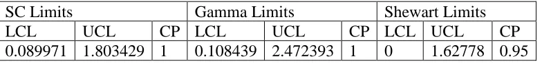
The skewness for this data is -0.16846. We have used the interpolated control chart constant values based on skewness correction method from Tables 2.1 and 2.2, for the construction of Mean and Range charts. The exact limits of gamma are calculated using the constants of Table 3.1. The coverage probabilities and average run length values for the mean and range charts are given in the following table.
Mean Chart:
SC Limits Gamma Limits Shewart Limits
LCL UCL CP (ARL) LCL UCL CP(ARL) LCL UCL CP(ARL)
2.051186 2.944386 0.95 (11th
Observation)
2.277995 4.221783 0.95 (17th
Observation)
2.06971 2.95829 0.55 (17th
Observation)
Range Chart:
SC Limits Gamma Limits Shewart Limits
LCL UCL CP LCL UCL CP LCL UCL CP
delayed alert of out of control indicating that mechanical usage of Shewart limits for non-normal data results in admissible conclusions.
References
1. Amin, R.W., and Miller, R.W. (1993). A Robustness Study of 𝑋̅ Charts with Variable Sampling Intervals. Journal of Quality Technology, Vol. 25, No. 1, 36-44.
2. Amin, R.W., and Oskar Widmaier. (1999). Sign Control Charts with Variable Sampling Intervals. Communications in Statistics – Theory and Methods, Vol. 28, No. 8, 1961-1985.
3. Chan, L.K., and Cui, H.J. (2003). Skewness Correction 𝑋̅ and R Charts for Skewed Distributions. Naval Research Logistics, Vol. 50, 1-19.
4. Costa, A.F.B. (1995). 𝑋̅ Charts with Variable Sample Size. Journal of Quality Technology, Vol. 26, 155-163.
5. Costa, A.F.B. (1996). Joint 𝑋̅ and R Charts with Variable Sample Sizes and Sampling Intervals. Technical Report # 142, Center for Quality and Productivity Improvement. University of Wisconsin, Madison.
6. Derya, K., and Canan, H. (2012). Control Charts for Skewed Distributions: Weibull, Gamma, and Lognormal. Metodoloṧki Zvezki, Vol. 9, No. 2, 95-106. 7. Edgeman, R.L. (1989). Inverse Gaussian Control Charts. Australian Journal of
Statistics, Vol. 31, No. 1, 78-84.
8. Göb, R., Ramalhoto, M.F., and Pievatol, A. (2006). Variable Sampling Intervals in Shewhart Charts Based on Stochastic Failure Time Modelling. Quality Technology & Quantitative Management, Vol. 3, No. 3, 361-381.
9. Kan, B., and Yazici, B. (2006). The Individuals Control Charts for Burr Distributed and Weibull Distributed Data. WSEAS Transactions on Mathematics, Vol. 5, No. 5, 555-561.
10. Kantam, R.R.L., and Priya, M.Ch. (2010). Extreme Order Statistics- Control Charts, ANU Journal of Physical Sciences, Vol. 2, No. 1, 48-55.
11. Kantam, R.R.L., and Priya, M.Ch. (2011). Time Control Charts Using Order Statistics, Interstat, September.
12. Kantam, R.R.L., and Srinivasa Rao, B. (2010). An Improved Dispersion Control Chart for Process Variate. International Journal of Computational Mathematical Ideas, Vol. 2, No. 1 & 2, 82-92.
13. Kantam, R.R.L., and Sriram, B. (2001). Variable control charts based on Gamma distribution, IAPQR Transactions, Vol. 26, No. 2, 63 - 77.
14. Kantam, R.R.L., Vasudeva Rao, A. and Srinivasa Rao, G. (2006). Control Charts for log-logistic distribution, Economic Quality Control, Vol. 21, No. 1, 77 - 86. 15. Mahadik, S.B., and Shrike, D.T. (2007). On the Superiority of a Variable
16. Srinivasa Rao, B., and Kantam, R.R.L. (2012). Mean and Range Charts for Skewed Distributions- A Comparison Based on Half Logistic Distribution, Pakistan Journal of Statistics, Vol. 28, No. 4, 437-444.
17. Wu, C., Zhao, Y., and Wang, Z. J. (2002). The Median Absolute Deviation and their Applications to Shewhart 𝑋̅ Control Charts. Statistical Simulation, Vol. 31, No. 3, 425-442.