www.solid-earth.net/7/229/2016/ doi:10.5194/se-7-229-2016
© Author(s) 2016. CC Attribution 3.0 License.
On the thermal gradient in the Earth’s deep interior
M. Tirone
Institut für Geologie, Mineralogie und Geophysik, Ruhr-Universität Bochum, 44780 Bochum, Germany Correspondence to: M. Tirone ([email protected])
Received: 19 August 2015 – Published in Solid Earth Discuss.: 8 September 2015 Revised: 14 January 2016 – Accepted: 20 January 2016 – Published: 10 February 2016
Abstract. Temperature variations in large portions of the mantle are mainly controlled by the reversible and irre-versible transformation of mechanical energy related to pres-sure and viscous forces into internal energy along with diffu-sion of heat and chemical reactions. The simplest approach to determine the temperature gradient is to assume that the dynamic process involved is adiabatic and reversible, which means that entropy remains constant in the system. How-ever, heat conduction and viscous dissipation during dynamic processes effectively create entropy. The adiabatic and non-adiabatic temperature variation under the influence of a con-stant or varying gravitational field are discussed in this study from the perspective of the Joule–Thomson (JT) throttling system in relation to the transport equation for change of en-tropy. The JT model describes a dynamic irreversible pro-cess in which entropy in the system increases but enthalpy remains constant (at least in an equipotential gravitational field). A comparison is made between the thermal gradient from the JT model and the thermal gradient from two models, a mantle convection and a plume geodynamic model, cou-pled with thermodynamics including a complete description of the entropy variation. The results show that the difference is relatively small and suggests that thermal structure of the asthenospheric mantle can be well approximated by an isen-thalpic model when the formulation includes the effect of the gravitational field. For non-dynamic or parameterized man-tle dynamic studies, the JT formulation provides a better de-scription of the thermal gradient than the classic isentropic formulation.
1 Introduction
In the Earth’s deep interior, dynamic processes involving large pressure variations induce temperature changes that of-ten are approximately described by an adiabatic gradient. The transformation of pressure–volume mechanical work into thermal heat is strictly considered adiabatic when there is no exchange of heat between the system and the surround-ings, δq=0. The common simplification applied to solid Earth problems is that the process is also reversible, hence the transformation is isentropic (Lewis and Randall, 1961; Denbigh, 1971; Sandler, 1988; Turcotte and Schubert, 1982; Schubert et al., 2001). The reversible condition is in most cases an approximation; in fact, spontaneous or natural pro-cess are intrinsically irreversible, therefore dSis usually not zero (Lewis and Randall, 1961; Denbigh, 1971; Zemansky et al., 1975; Sandler, 1988). The irreversible entropy pro-duction in the mantle comes from various sources, mainly from heat conduction transformation of mechanical energy into internal energy by viscous forces (viscous dissipation) and chemical reactions. While determination of the entropy production from all these effects may require a full-scale dy-namic thermal model (e.g Bird et al., 2002), an alternative is given by the description of the throttling process designed by the Joule–Thomson (JT) experiment (e.g. Zemansky et al., 1975) which is usually referred to as a typical example of an isenthalpic process and has been extensively discussed in the geological context by Ganguly (2008).
mantle upwelling which also extended to melting processes was presented by Ganguly (2005).
However, some questions remain in particular as to whether the JT model is better suited than the isentropic for-mulation to describe the thermal gradient in the mantle. In addition the difference in terms of thermal or entropy change with the complete entropy description from a dynamic ther-mal model has not been quantified yet.
In Sect. 2 the thermodynamic and heat transport formula-tion is presented with focus on the entropy change and the connection to the JT formulation. In Sects. 3 and 4 a 2-D mantle convection and a 2-D thermochemical plume model combined with a chemical equilibrium approach (Gibbs free energy minimization) are used to determine the entropy-related term and the irreversible thermal contribution. The result is then compared with the JT thermal model in order to understand whether the JT formulation could provide a rea-sonable description of the thermal structure of the mantle. The general outline of the numerical computation of the adi-abatic thermal gradient (reversible and irreversible) in com-bination with a chemical equilibrium approach is described in Sect. 5, along with a series of mantle geotherms to illus-trate the effect of the irreversible entropy production based on the JT formulation. Numerical details can be found in the Appendix.
2 Thermodynamic and transport formulation of thermal change
This section presents the formulation for the entropy change in relation to heat conduction and viscous dissipation in transport models and the relation that needs to be fulfilled for a process to be assimilated to the JT model. The gen-eral expression for the entropy change of a moving fluid in a quasi-equilibrium state is given by Bird et al. (2002): ρDS
Dt = −∇ · q
T +σ, (1)
whereSis the entropy per unit mass, D/Dtis the substantial derivative; the first term on the right-hand side (rhs) is the rate of entropy increase by heat conduction and the second term σ is the entropy production. The first law of thermodynamics dU=TdS−PdV for a small mass moving with the fluid is
DU Dt =T
DS Dt −P
DV
Dt (2)
and the transport equation for the internal energy is given by the following (Bird et al., 2002):
ρDU
Dt = −∇ ·q−P∇ ·v−τ: ∇v, (3) where the first term on the rhs is the rate of energy change by heat conduction, the second term is the reversible energy change by volume compression/expansion and the last term
is the irreversible energy increase by viscous dissipation, as-suming a Newtonian fluid with velocityvand viscous stress tensorτ. Inserting DS/Dtfrom Eq. (1) in (2) and combining the relation for DU/Dt with Eq. (3):
−T∇ · q
T +T σ−ρP DV
Dt = −∇ ·q−P∇ ·v−τ : ∇v. (4) Using the relationP∇ ·v=ρPDV /Dt(Sandler, 1988) and the relation
∇ ·q
T = 1
T∇ ·q+q· ∇ 1
T (5)
in Eq. (4), the entropy productionσcan be defined as σ=q· ∇1
T − 1
Tτ: ∇v. (6)
The effect of chemical transformations and other potential sources of entropy are ignored for simplicity or because they are negligible in the mantle (electric resistance, magnetic field, non-Newtonian fluid). The equation of change for tem-perature for a mass moving with the fluid can be obtained from Eq. (1) by replacing σ with the expression given in Eq. (6) and the thermodynamic relation for dSas a function ofP,T, dS=Cp/TdT −αVdP:
ρCp
DT
Dt = −∇ ·q−τ : ∇v+αT DP
Dt , (7)
where ρ=1/V has been applied. This is the standard description of temperature change that, for an inviscid fluid under adiabatic and time- and space-invariant condi-tions, describes an isentropic thermal gradient (dT /dP|S=
αV T /Cp).
In the well-known Joule–Thomson experiment (e.g. Ze-mansky et al., 1975; Callen, 1985; Ganguly, 2008) a gas steadily flows from one subsystem to another subsystem through a porous plug. The plug avoids turbulent flow and inhomogeneous pressure distribution in both subsystems. The entire system (made of the two subsystems) is con-fined on both ends by two moving pistons. The pistons quasi-statically keep a predefined pressure on both sides. The whole system is thermally insulated and mass is con-served. The thermodynamic analysis shows that the process is isenthalpic, dH=0 (Lewis and Randall, 1961; Denbigh, 1971; Zemansky et al., 1975; Callen, 1985). We can express the equation of change for the internal energy (Eq. 3) as a function of the enthalpy change by replacing DU/Dt with DH /Dt−D(P V )/Dt:
ρDH
Dt = −∇ ·q−τ : ∇v+ DP
Dt , (8)
where the relationP∇ ·v=ρD(P /ρ)/Dt−DP /Dthas been used. Therefore for an isenthalpic process (DH /Dt=0) Eq. (8) establishes the relation
DP
or using the expression for the entropy production Eq. (6): DP
Dt = −T σ+T∇ · q
T. (10)
Both relations show the necessary condition that must hold for an isenthalpic process. The isenthalpic condition can be verified by using Eq. (10) in the equation of change for tem-perature (Eq. 7) to find the equation of change for temper-ature ρCpDT /Dt=(αT−1)DP /Dt which, in differential
form, reproduces the well-known isenthalpic thermal gradi-ent dT /dP|H=(αT−1)/(ρCp)(Ramberg, 1971; Ganguly,
2008). The same relation between pressure and the entropy production (Eqs. 9 and 10) can be also obtained by express-ing the thermodynamic relation given in Eq. (2) in terms of enthalpy as DH /Dt=TDS/Dt+VDP /Dt. Assuming the isenthalpic condition, we have
TDS Dt = −V
DP
Dt , (11)
then Eq. (10) can be found by using Eq. (1) to replace DS/Dt in the above expression.
In a varying gravitational field, the isenthalpic condition should be replaced by dH=VdPg(Dodson, 1971; Ramberg,
1971), where dPg=ρgdz. Then the expression for entropy
equivalent to Eq. (11) is
TDS Dt =V
DP
g
Dt − DP
Dt
(12) and the equivalent to Eq. (9) relating the pressure changes to entropy changes is
DP Dt −
DPg
Dt = ∇ ·q+τ: ∇v. (13)
The dynamic thermal model (Eq. 7) is not affected by these two equations, however if the conditions are such that in Eq. 13 the difference of the pressure changes on the left-hand side (lhs) and the entropy-related terms on the rhs are close to be equal, then the thermal process can be assim-ilated to a JT model in a varying gravitation field. If this is the case, Eq. (12) can be used to find the thermal gradi-ent for the JT model including the gravitational effect. Un-der space- and time-invariant conditions, Eq. (12) reduces to TdS=VdPg−VdP, and by expressing the entropy change
dS as dS=Cp/TdT −αVdP, the thermal gradient can be
described by the following equation: dT
dP
H
g
=(αT−1)V
Cp
+ 1
Cp
dPg
dP . (14)
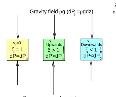
The interesting aspect of the JT thermal model is that a pres-sure gradient (difference), which fundamentally defines dy-namic flow, is naturally included. In addition entropy in-creases only when the pressure is not equal to the pressure generated by the gravitational fieldPg. The pressure change
z=0
Gravity field
ρ
g (dP
g=
ρ
gdz)
P, pressure on the system
vz=0 vz
Downwards vz
Upwards
dP=dP
g+
dP<dP
gdP>dP
gξ
< 1
ξ
= 1
ξ
> 1
Figure 1. Vertical pressure components acting on the system.
Ver-tical motion is the result of the difference between the gravitational pressure forcePgand the vertical pressure force P acting on the system.
can be related to the gravitational pressure by a scaling fac-torζ so that dP =ζρgdz=ζdPg. Using this scaling factor
in Eq. (14), the following expression for temperature changes with depth under adiabatic irreversible conditions in a vary-ing gravitational field is
dT dz
H
g = g
Cp
(1−ζ )+ζ
gT α Cp
. (15)
This equation is the same as the corresponding expression derived by Ganguly (2005, Eq. 16) after settingζ =ρr/ρ,
whereρris the density of the ambient mantle at rest (so that
dP =ρrgdz), and the acceleration term is ignored. Using the
scaling factorζ, the irreversible entropy production assumes the following form:
dS= −VdPg(ζ−1)/T . (16)
The condition of hydrostatic equilibrium is obtained when ζ=1 and no entropy is produced. Ifζ >1 (pressure gradi-ent is greater than the gradigradi-ent of the gravitational pressure), the system moves upwards (Fig. 1). Noticeably the increase of entropy moving upwards (dS/dz <0) is consistent with a spontaneous process. Conversely, whenζ <1, entropy in-creases at greater depths (dS/dz >0) and the material spon-taneously moves downwards.
3 Mantle geotherms in a convective mantle
to the extent that would justify the use of the JT model to de-scribe the thermal gradient in the mantle. The results summa-rized in Fig. 2 are based on a 2-D compressible flow model heated from below and coupled to a thermodynamic formu-lation associated with Saxena’s database (Saxena, 1996) in the system MgO–FeO–SiO2 to computed density and heat
capacity. The oxides’ abundance, defined as MgO=44.72, FeO=9.48, SiO2=45.8 (wt %), approximately describes a peridotite bulk composition. The dynamic transport equa-tions for a compressible flow can be found in Schubert et al. (2001). The details of the numerical solution are given in Tirone et al. (2009). Viscosity is set to (1×10²²Pa s), ther-mal conductivity is 3 W m−1K−1 and the bottom tempera-ture is 3327◦C. The temperature at the base of the model is set in a way that the model does not create an unreal-istic exceedingly hot upper mantle. The dynamic thermal model does not include any viscous dissipation or adiabatic reversible terms in the transport equation which is simply given byρCpDT /Dt= −∇ ·q. The additional terms in the
thermal equation are computed in a second stage using the parameters from the dynamic model. This simplified ap-proach implies that there is no coupling between the param-eters used to compute the thermal gradients and the com-puted thermal gradients. On the right middle panel of Fig. 2, the terms (v·(∇P− ∇Pg)) and (∇ ·q+τ: ∇v) are used
to assess whether the irreversible contribution to the ther-mal gradient from the JT model is comparable to the irre-versible effect from heat conduction and viscous dissipation (see Eq. 13) along the upwelling and downwelling flow di-rections. Assuming a steady state, the vertical component of the thermal effect 1Tz added to the isentropic gradient is given by the integration of (v·(−∇P+ ∇Pg))1z/(ρCpvz) and(−∇ ·q−τ : ∇v)1z/(ρCpvz)for the JT model and gen-eral entropy case respectively. The result for the downwelling and upwelling flow are shown in the lower panel of Fig. 2. For this particular mantle convection model it appears that the difference between the two thermal gradients is quite small. It is also quite evident that the JT model is a better rep-resentation of the thermal variations than the one offered by the isentropic formulation. The ratio between the flow pres-sure and the gravitational prespres-surePgalong two vertical
sec-tions extracted from the model (middle left panel of Fig. 2) is the necessary information that can be used to compute the JT thermal gradient in non-dynamic models (see Sect. 5).
4 Thermal gradient of a mantle plume
In this section, a detailed geodynamic model of a thermal plume is used for a further comparison with the thermal gra-dient given by the JT model. The general description of the coupling between the geodynamic model and the thermo-dynamic formulation has been discussed elsewhere (Tirone et al., 2009). The transport equation for temperature change in this model includes an additional heat source term to
de-0 2000 km 4000 6000
0
1000
2000
3000
D
e
p
th
(k
m
)
1955.56 1866.67 1777.78 1688.89 1600
T (o C) > 2000
< 1600
TIME= 167.5000 Ma
0.98 0.99 1 1.01 1.02
P/Pg 500
1000
1500
2000
2500
3000
Downwelling Upwelling Depth(km)
1800 2000 2200 2400 2600 Temperature (o
C) 0
500
1000
1500
2000
2500
3000
D
e
p
th
(k
m
)
Reversible
Irreversible
Upwelling
Irreversible JTg
1200 1400 1600 1800 2000
Temperature (o C) 0
500
1000
1500
2000
2500
3000
D
e
p
th
k
m
Reversible
Irreversible JTg
Downwelling
Irreversible
-1E-06 0
500
1000
1500
2000
2500
3000
Depth(km)
(∇⋅q+
τ:∇⋅v)down
v⋅(∇
P-∇Pg)down v⋅(∇
P-∇Pg)up
(∇⋅q+τ:∇⋅v)up
v⋅(∇P-∇Pg) and (∇⋅q+τ:∇⋅v) (kg m -1
s-3 )
Figure 2. The upper panel shows temperature for an isoviscous
mantle convection simulation (heated from below) coupled with a thermodynamic model. Temperature at the bottom is set to 3327◦C. In the geodynamic model the thermal field does not in-clude the reversible adiabatic and viscous dissipation effects. The middle left panel shows the ratio between the flow pressure and the gravitational pressurePg=ρgdz. The middle right panel shows the irreversible contribution to the thermal gradient given by heat conduction and viscous dissipation (solid lines) and the irreversible contribution in the JT formulation including the gravitational ef-fect (dashed lines; see Eq. 13). The lower panel shows the thermal gradient computed from the isentropic formulation (reversible), the irreversible formulation by adding heat conduction and viscous dis-sipation (irreversible) and the JT formulation with gravity (dashed lines, irreversible JTg).
scribe the contribution of chemical transformations: ρCp
DT
Dt = −∇ ·q−τ : ∇v+αT DP
Dt +T ρ
X
Si Dni
ad-vective vertical component. The temperature at the bottom of the 2-D numerical model is set to 2827◦C. This tempera-ture has been chosen a posteriori based on the thermal struc-ture of the plume in the upper mantle that should not be too far off from the thermal conditions for melting a dry peri-dotite. The viscosity is defined by a model which depends on pressure, temperature and mineralogical assemblage. Ther-mal conductivity in the upper mantle is set to 4 W m−1K−1. In the lower mantle the thermal conductivity is defined by the model of Manthilake et al. (2011), and assumes the follow-ing form:k=4.7(700/T )0.21(ρ/4400)4. The numerical grid spacing is 1x=10 km,1z=10. All other parameters that are needed in the dynamic model are defined by the ther-modynamic formulation using Saxena’s database (Saxena, 1996) supplemented with the thermodynamic parameters for post-perovskite (ppv), retrieved by summarizing several ex-perimental data and previous studies (Murakami et al., 2004; Tsuchiya et al., 2005; Hirose, 2006; Shieh et al., 2006; Spera et al., 2006; Tateno et al., 2007; Komabayashi et al., 2008; Shim, 2008; Andrault et al., 2010; Dorfman et al., 2013).
The thermodynamic parameters for MgSiO3-ppv and FeSiO3-ppv are as follows:
– (MgSiO3-ppv) reference enthalpy, entropy and molar volume at 300 K, 1 bar: 1Hf(Tr, Pr)= −1 405 894
(j mol−1), S(Tr, Pr)=77.60 (j mol−1K−1),
v0(Tr, Pr)=2.4447 (j mol−1bar−1); heat
ca-pacity coefficients: k1=139.7, k2=0.8300e-5,
k3= −4 410 000, k4=0, k5=0.1038e9, k6=0,
k7= −10 346; thermal expansion coefficients:
a1=4.4084e-5, a2= −8.8066e-10, a3= −
0.8967e-2, a4=1.4107; bulk modulus coefficients:
v1=232.3e4, a2= −0.2885e3, v3=1.4162e-2
and dK/dP (T =300 K)=3.84,d2K/dPdT =1e-5; – (FeSiO3-ppv) reference enthalpy, entropy and molar
volume at 300 K, 1 bar: 1Hf(Tr, Pr)= −1 059 880
(j mol−1), S(Tr, Pr)=64.07 (j mol−1K−1),
v0(Tr, Pr)=2.7382 (j mol−1bar−1); heat
ca-pacity coefficients: k1=139.7, k2=0.8300e-5,
k3= −4 410 000, k4=0, k5=0.1038e9, k6=0,
k7= −10 346; thermal expansion coefficients:
a1=4.4084e-5, a2= −8.8066e-10, a3= −
0.8967e-2, a4=1.4107; bulk modulus coefficients:
v1=153.7e4, a2= −0.2885D3, v3=1.4162e-2
and dK/dP (T =300 K)=4.24,d2K/dPdT =5.2e-5. The following equations apply for heat capacity (1 bar): Cp=k1+k2T +k3/T2+k4T2+k5/T3+k6/T1/2+k7/T
(j mol−1K−1); thermal expansion (1 bar) α=a1+a2T+
a3 / T +a4/T2 (K−1); bulk modulus (1 bar) K=v1+
v2T +v3T2(bar); derivative of the bulk modulus with
pres-sure (1 bar) dK/dP =dK/dP (300 K)+d2K/dPdT (T−
300)ln(T /300). Mixing between Mg-ppv and Fe-ppv is as-sumed to be ideal.
(km)
De
p
th
(k
m
)
0 1000 2000
0
500
1000
1500
2000
2500
3000
11001247.371394.741542.111689.471836.841984.212131.582278.952426.32
1100o
C < > 2500o
C
TCMB=2827 o C
Temperature ( C) o
De
p
th
(k
m
)
1750 2000 2250 2500 2750
0
500
1000
1500
2000
2500
3000 T
CMB= 2827 o
C Pv + Mg-Wu
PPv Pv
Wd Rw Ol
Reversible Irreversible
Irreversible JTg
v⋅(∇P-∇Pg) and (∇⋅q+τ:∇⋅v)(kg m -1
s-3 )
De
p
th
(k
m
)
-3E-06 -2E-06 -1E-06 0 1E-06
0
500
1000
1500
2000
2500
3000
v⋅(∇P-∇Pg)
(∇⋅q+τ:∇⋅v) P/Pg
De
p
th
(k
m
)
1 1.005 1.01 0
500
1000
1500
2000
2500
3000
TIME= 0.0000 Ma
TIME= 0.0000 Ma
TIME= 0.0000 Ma
Figure 3. The top left panel shows the dynamic model of a thermal
plume coupled with a thermodynamic formulation, including the ir-reversible effect of heat conduction, viscous dissipation and chem-ical transformations. The right panel shows the comparison of the thermal profile along the plume vertical section between the numer-ical model that includes the irreversible effects (from the simulation shown on the left panel) and the thermal gradient including the JT irreversible effect (dashed line). The reversible thermal profile is ob-tained by subtracting the integral of(−∇ ×q−τ: ∇v)1z/(ρCpvz)
from the dynamic thermal model. The lower left panel shows the ratio between the flow pressure and the gravitational pressure. The lower right panel shows the irreversible contribution to the thermal gradient given by heat conduction and viscous dissipation for the plume model (solid line) and irreversible contribution in the JT for-mulation, including the gravitational effect (dashed line).
1500 2000 2500 T(o
C)
500
1000
1500
2000
2500
3000
D
e
p
th
(k
m
)
ζ=1.005
Cp(P)5e5
ζ=1.01
ζ=1.02
ζ=0.98
Cp(P)1e6
Downwelling Upwelling
ζ=1
ζ=1
ζ=0.99
2.3 2.4 2.5 2.6S (J Kg2.7 2.8 2.9 3 -1
K-1)
500
1000
1500
2000
2500
3000
D
e
p
th
(k
m
)
Downwelling Upwelling
ζ=0.98
ζ=1.005
ζ=0.99
ζ=1
ζ=1
ζ=1.01
ζ=1.02
Figure 4. The upper panel shows the reversible and JT irreversible
adiabatic temperature gradients in the Earth’s mantle for upwelling (T at the bottom is 2727◦C) and downwelling (T at the top is 1150◦C). The lower panel shows the change of entropy with depth. All cases assume the heat capacity at 1 bar except the profiles with the labelCp(P )(see main text for further details). Bold lines high-light the isentropic case.
thermal profiles are very similar; in fact, the change of the entropy-related terms (lower right panel, Fig. 3) is quite sim-ilar. Oscillations in particular at the pv–ppv boundary and around the transition zone are the consequence of the effect of the chemical transformations on the numerical computa-tion of the heat flux and pressure gradients. The pressure ratio P /Pg(lower left panel) can be used to compute the thermal
gradient based on the JT model without performing a full-scale dynamic simulation, as shown in the next section.
5 Mantle geotherms
The computation of the adiabatic thermal gradient in the Earth’s deep interior involves the determination at discrete depth intervals of (1) temperature, (2) pressure and (3)
equi-librium mineralogical assemblage. The numerical details rel-ative to the computation of the temperature from the relevant thermodynamic quantities are discussed in the Appendix. The thermodynamic properties and bulk composition have been defined in the previous sections. The whole algorithm can be briefly summarized as follows. With an initial guess of the density at each grid point, the gravitational pressure is computed starting at the uppermost point where the pressure and depth are predefined. Then, after computing the entropy, enthalpy and the additional functionsS∗andH∗at the deep-est point (Eqs. A1–A4, and A5, in Appendix A), the com-putation of the functionsS∗ and H∗ (Eq. A12 forS∗ and similar forH∗) is combined with a Gibbs free energy min-imization to determine the equilibrium assemblage and the temperature at each grid point simultaneously. Once the ini-tial temperature profile versus depth has been determined, the gravitational pressure is re-evaluated with the updated den-sities along with pressure (using the scaling factorζ) and the procedure continues until no significant variations of the pressure at any depth are observed between two iterations.
The algorithm just outlined is applied to compute the adi-abatic gradient in the mantle convective region. The thermo-dynamic database for the system MgO–FeO–SiO2(Saxena,
1996) with the addition of data for post-perovskite (see pre-vious section) is used in the Gibbs free energy minimiza-tion and addiminimiza-tional thermodynamic calculaminimiza-tions. The depth at the bottom is 3000 km; the temperature at this depth is set to 2727◦C for the upwelling. This starting temperature is within a reasonable range, consistent with the expected inter-section of the plume temperature with the solidus of a peri-dotite in the upper mantle. For the downwelling thermal gra-dient the depth at the top is 200 km; at this point the pressure is set to 62 kbar and the temperature is fixed at 1150◦C. It should represent the temperature at some intermediate depth in a hypothetical subducting slab. This is all the information needed to compute the isentropic adiabatic gradient. To eval-uate the irreversible adiabatic effect, the scaling factorζ re-latingP toPghas to be specified, e.g. lower than 1.0 in case
of mantle upwelling and greater than 1.0 in case of down-ward flow. For simplicity it is assumed to be constant at any depth, although it can vary, as has been shown in the previ-ous sections. Figure 4 summarizes the results. On the upper panel the isentropic geotherm is plotted, along with a series of irreversible geotherms for upwelling which show that the adiabatic thermal gradient gets steeper as the scaling factor increases. These geotherms are computed, taking the heat ca-pacity value at the given temperature and 1 bar. As discussed in Appendix A this is not exactly correct. Two additional isentropic geotherms are computed assuming a linear pres-sure dependence of the heat capacity from 1 bar to a prede-fined limit pressure (set to 500 and 1000 kbar) at whichCp
is the value of the heat capacity at the Dulong–Petit limit. The linear assumption should at least give a qualitative sense of the pressure effect on the heat capacity and the geotherm. The result in Fig. 4 for the isentropic case (ζ =1) suggests a decrease of the thermal gradient. The lower panel of Fig. 4 illustrates the entropy production for the irreversible cases. Geotherms are also computed for downwelling, assuming an isentropic gradient and two irreversible gradients with ζ equal to 0.99 and 0.98. The effect of the irreversible entropy production in this case is to decrease the thermal gradient.
The JT model seems to offer a better estimate of the ther-mal structure than the isentropic model because it accounts, to a large extent, for the entropy increase that would be ob-served from a full-scale dynamic thermal model.
6 Conclusions
The main objective of this study is to better understand whether the irreversible entropy production in the dynamic mantle can be assimilated to the entropy related to the JT model. This appears to be the case based on the two geody-namic models used in this study; in fact the thermal structure of the mantle could be assumed to follow, to a large extent, an isenthalpic model when the gravitational effect is included. The thermal gradient is closely related to the thermal gradi-ent that would be obtained by a full-scale dynamic thermal model, therefore the model represents a better alternative to the isentropic formulation when applied to non-dynamic or parameterized thermal models. The formulation based on the JT model is relatively simple and, in comparison to the isen-tropic formulation, requires only one additional term (scaling factorζ or pressure ratio).
Appendix A: Numerical procedure to compute the adiabatic thermal gradient
The chemical equilibrium computation is based on a Gibbs free energy minimization in which pressure, temperature and bulk composition are given as input quantities. Gravitational pressure is determined by the numerical integration ofρgdz, where the density is known from the equilibrium mineralogi-cal assemblage. The computational procedure starts by eval-uating the molar entropy and the enthalpy of the system at the deepest point where temperature is assumed to be known:
Sm(Pb, Tb)=Sm(1 bar,298 K)+
Tb
Z
298 K
CPm
T dT 1 bar − Pb Z 1 bar
αmVmdP Tb (A1)
Hm(Pb, Tb)=Hm(1 bar,298 K)+
Tb
Z
298 K
CPmdT
1 bar + Pb Z 1 bar
VmdP Tb −Tb
Pb
Z
1 bar
αmVmdP Tb , (A2)
where the subscript b stands for the bottom point and the subscript m for the molar properties of a particular min-eral component in the equilibrium assemblage. Two addi-tional quantitiesS∗orH∗, derived from the relations dS∗= Cp/TdT−αVdP+V /TdP−Vρg/Tdzand dH∗=CpdT+
(1−αT )VdP−Vρgdz, are also computed at the bottom point:
Sm∗(Pb, Tb)=Sm∗(1 bar,298 K)+
Tb
Z
298 K
CPm
T dT 1 bar (A3) − Pb Z 1 bar
αmVmdP Tb + 1 Tb Pb Z 1 bar
VmdP Tb − 1 Tb Pgb Z 1 bar
VmdPg T b and
Hm∗(Pb, Tb)=Hm∗(1 bar,298 K)+
Tb
Z
298 K
CPmdT
1 bar (A4) + Pb Z 1 bar
VmdP Tb −Tb
Pb
Z
1 bar
αmVmdP Tb −
Pgb
Z
1 bar
VmdPg T b ,
where dPg, is defined asρgdz. The relation between dP and
dPg, introduced in Sect. 2, is dP =ζdPgandζ is the
prede-fined scaling factor. The total thermodynamic properties are
evaluated using φ (P , T )=X
m
nmφm(P , T ), (A5)
whereφisS,H,S∗orH∗, andnis the number of moles of the component at equilibrium obtained from the Gibbs free energy minimization. The functionsS∗andH∗are the refer-ence quantities that need to be maintained constant at every depth point. To evaluate these quantities at any depth, the starting point is the differential expression of the total prop-erties:
dS=X m
nm
C
Pm
T dT−αmVmdP
+X
m
Smdnm (A6)
dH=X m
nm CPmdT +(1−αmT )VmdP
+X
m
Hmdnm (A7)
dS∗=X m
nm
C
Pm
T dT−αmVmdP+ Vm
T dP− Vm
T dPg
+X
m
Smdnm (A8)
dH∗=X m
nm CPmdT +(1−αmT )VmdP−VmdPg
+X
m
Hmdnm. (A9)
The equations are integrated over two depth intervals, for ex-ample fromz+1 toz. Integration ofS∗(Eq. A8) gives S∗(Pz, Tz)=
X m
nmzS ∗
mz=
X m
nmz+1S
∗
mz+1+
X m
nmz
(
CPmz Tz
(Tz−Tz+1)
(Pz+1)
− Pz Z 1 bar
αmVmdP−
Pgz+1
Z
1 bar
αmVmdPg
− 1 Tz Pz Z 1 bar
VmdP−
Pgz+1
Z
1 bar
VmdPg (Pz) +X m
Smz+1(nmz−nmz+1)|(Tz+1,Pz+1), (A10)
where the integration over the moles of the components is done atPz+1, Tz+1, the integration over temperature from
Tz+1toTzatnz,Pz+1and the integration over pressure from
Pz+1toPzatnz,Tz. The integral over pressure is better eval-uated as the difference between the integral from 1 bar toP atzand from 1 bar toP atz+1. The above equation can be rearranged using the relation
Smz+1=S
∗
mz+1− 1
Tz+1
z+1
Z
z+2
VmdP−
z+1
Z
z+2
VmdPg
(z+1)
and the final expression forS∗atzafter some substitutions is
S∗(Pz, Tz)=
X m
nmzS ∗
mz+1
+X
m
nmz
. . .
+X
m
(Smz−Smz+1)(nmz−nmz+1), (A12)
where the quantity within the brackets{. . .}is the same as in Eq. (A10). The integrals with the heat capacity at 1 bar in Eqs. A3 and A4 and the integration of the volume at T (Eqs. A3, A4, A10–A12) are solved analytically. The inte-gration ofαV over pressure is solved numerically. At a given temperature the numerical integration using the trapezoidal rule (Press et al., 1997) is
P
Z
1 bar
αVdP
T ≈
X
Pi
α1 bar
(VPi−1+VPi)
2 +
(VPi−11αPi−1+VPi1αPi)
2
!
T
1P, (A13) where the index for the molar properties has been dropped for simplicity. The summation is over an arbitrary pressure grid (1P =20 kbar) from 1 bar to the final pressureP. The quan-tity defined as1αis the pressure contribution to the thermal expansion which is computed numerically at a certain pres-sure using the following reciprocity relation (Denbigh, 1971) in discretized form (1T =10◦C):
∂α ∂P
T ,Pi
≈ 1
KT ,Pi2
!
(KT+1T ,Pi−KT−1T ,Pi)
21T (A14)
and then
1αi≈1αi−1+
∂α ∂P
T ,Pi + ∂α
∂P
T ,Pi+1
2 1P , (A15)
where1αi is the total change of thermal expansion due to the pressure effect from 1 bar toPi.
To evaluate S∗, the heat capacity in Eq. (A10) and sim-ilarly in the expressions for H∗,S andH should be com-puted at the pressure and temperature associated with the depth point z+1. However, the thermodynamic database (Saxena, 1996) is not suitable for precise evaluation of the pressure dependence ofCp(via integration of dCp/dP|T = −Td2V /dT2|P, Lewis and Randall, 1961). This is a com-mon problem of existing databases (Jacobs et al., 2006; Tirone, 2015). The simplest but crude approximation is to take the heat capacity at 1 bar and at the given temperature. An alternative is that one can assume a linear pressure de-pendence between the heat capacity at 1 bar and the Dulong– Petit limit at some predefined high pressure value. This is
based on the observation that at high pressure and temper-ature,CpandCvapproach the Dulong–Petit value (Tirone,
2015). Both cases have been considered for the evaluation of a mantle geotherm in Sect. 5.
The temperature that maintains the functionsS∗andH∗ at a constant level is found using a simple bisection method (Press et al., 1997). The whole algorithm is applicable for a reversible or irreversible adiabatic volume change. As men-tioned in Sect. 2 when the scaling factor ζ is set to 1.0, S∗ (Eq. A3) reduces to the standard definition of entropy (Eq. A1) andH∗is such that dH∗=CpdT−αV TdP =0.
One could imagine evaluating the thermodynamic properties at any depth following the same integration scheme from 1 bar, 298 K, that was applied for the bottom depth point (Eqs. A1–A5) instead of applying Eq. (A12). However for comparison with the reference bottom point value, it would have been necessary to carry on the slightly more difficult in-tegration of the molar change term (for example for S orS∗, the expressionP RS
mdnmat the finalP , T).
Acknowledgements. This work benefited from discussions
devel-oped over several years with J. Ganguly. Clarity of some of the concepts presented in this study was greatly improved thanks to the feedback from the students of a graduate course in thermody-namics and geodythermody-namics that has been offered at the Institut für Geologie, Mineralogie und Geophysik, Ruhr-Universität Bochum (2013–2015). Constructive comments of an anonymous reviewer and support of the topical editor (J. Afonso) are greatly appreciated.
Edited by: J. C. Afonso
References
Andrault, D., Muñoz, M., Bolfan-Casanova, N., Guignot, N., Per-rillat, J.-P., Aquilanti, G., and Pascarelli, S.: Experimental evi-dence for perovskite and post-perovskite coexistence throughout the whole D region, Earth Plan. Sc. Lett., 293, 90–96, 2010. Bird, R. B., Stewart, W. E., and Lightfoot, E. N.: Transport
Phenom-ena, 2nd Edn., John Wiley and Sons, New York, USA, 895 pp., 2002.
Callen, H. B.: Thermodynamics and an Introduction to Thermostat-ics, 2nd Edn., John Wiley and Sons, New York, USA, 493 pp., 1985.
Denbigh, K.: The Principles of Chemical Equilibrium: With Appli-cations in Chemistry and Chemical Engineering, 3rd Edn., Cam-bridge University Press, CamCam-bridge, UK, 494 pp., 1971. Dodson, M. H.: Isenthalpic flow, Joule–Kelvin coefficients and
mantle convection, Nature, 234, p. 212, 1971.
Dorfman, S. M., Meng, Y., Prakapenka, V. B., and Duffy., T. S.: Effects of Fe-enrichment on the equation of state and stability of (Mg,Fe)SiO3perovskite, Earth Plan. Sc. Lett., 361, 249–257, 2013.
Ganguly, J.: Thermodynamics: Principles and Applications to Earth and Planetary Sciences, 1st edn., Springer, Berlin, Germany, New York, USA, 719 pp., 2008.
Hirose., K.: Postperovskite phase transition and its geo-physical implications, Rev. Geophys., 44, RG3001, doi:10.1029/2005RG000186, 2006.
Jacobs, M. H. G., van den Berg, A., and de Jong, H. W. S: The derivation of thermo-physical properties and phase equilibria of silicate materials from lattice vibrations: Application to convec-tion in the Earth’s mantle, Calphad, 30, 131–146, 2006. Komabayashi, T., Hirose, K., Sugimura, E., Sata, N., Ohishi, Y., and
Dubrovinsky, L. S.: Simultaneous volume measurements of post-perovskite and post-perovskite in MgSiO3and their thermal equations of state, Earth Plan. Sc. Lett., 265, 515–524, 2008.
Lewis, G. N. and Randall, M.: Thermodynamics, 2nd Edn., Mc-Graw Hill, New York, USA, 723 pp., 1961.
Manthilake, G. M., de Koker, N., Frost, D. J., and McCammon, A.: Lattice thermal conductivity of lower mantle minerals and heat flux from Earth’s core, P. Natl. Acad. Sci. USA, 108, 17901– 17904, 2011.
McKenzie, D. and Bickle, M. J.: The volume and composition of melt generated by extension of the lithosphere, J. Petrol., 29, 625–679, 1988.
Murakami, M., Hirose, K., Kawamura, K., Sata., N., and Ohishi, Y.: Post-Perovskite phase transition in MgSiO3, Science, 304, 855– 858, 2004.
Press, W. H., Teukolsky, S. A., Vetterling, W. T., and Flannery, B. P.: Numerical Recipes in Fortran 77: The Art of Scientific Com-puting, 2nd Edn. (reprinted), Cambridge University Press, Cam-bridge, UK, 1486 pp. 1997.
Ramberg, H.: Temperature changes associated with adiabatic de-compression in geological processes, Nature, 234, 539–540, 1971.
Sandler, S. I.: Chemical and Engineering Thermodynamics, 2nd edn., Wiley, New York, USA, 622 pp., 1988.
Saxena, S. K.: Earth mineralogical model: Gibbs free energy mini-mization computation in the system MgO-FeO-SiO2, Geochim. Cosmochim. Acta, 60, 2379–2395, 1996.
Schubert, G., Turcotte, D. L., and Olson, P.: Mantle Convection in the Earth and Planets, 1st Edn., Cambridge University Press, Cambrige, UK, 940 pp., 2001.
Shieh, S. R., Duffy, T. S., Kubo, A., Shen, G., Prakapenka, V. B., Sata, N., Hirose, K., and Ohishi, Y.: Equation of state of the postperovskite phase synthesized from a natural (Mg,Fe)SiO3 or-thopyroxene, Proc. Natl. Acad. Sci. 103, 3039–3043, 2006. Shim, S.-H.: The Postperovskite Transition, Annu. Rev. Earth
Planet. Sci. 36, 569–599, 2008.
Spera, F. J.: Carbon dioxide in igneous petrogenesis: II. Fluid dy-namics of mantle metasomatism, Contrib. Mineral. Petr., 77, 56– 65, 1981.
Spera, F. J., Yuen, D. A., and Giles, G.: Tradeoffs in chemical and thermal variations in the post-perovskite phase transition: Mixed phase regions in the deep lower mantle?, Phys. Earth Planet Int., 159, 234–246, 2006.
Tateno, S., Hirose, K., Sata., N., and Ohishi, Y.: Solubility of FeO in (Mg,Fe)SiO3perovskite and the post-perovskite phase transition, Phys. Earth Planet Int., 160, 319–325, 2007.
Tirone, M.: On the use of thermal equations of state and the ex-trapolation at high temperature and pressure for geophysical and petrological applications, Geophys. J. Int., 202, 1483–1494, 2015.
Tirone, M., Ganguly, J., and Morgan, J. P.: Modeling petrological geodynamics in the Earth’s mantle, Geochem. Geophy. Geosy., 10, 1–28, 2009.
Tsuchiya, J., Tsuchiya, T., and Wentzcovitch, M.: Vibrational and thermodynamic properties of MgSiO3 postperovskite, J. Geo-phys. Res., 110, B02204, doi:10.1029/2004JB003409, 2005. Turcotte, D. L. and Schubert, G.: Geodynamics Applications of
Continuum Physics to Geological Problems, 1st edn., Wiley and Sons, New York, USA, 450 pp., 1982.
Waldbaum, D. R.: Temperature changes associated with adiabatic decompression in geological processes, Nature, 232, 545–547, 1971.