www.atmos-meas-tech.net/9/829/2016/ doi:10.5194/amt-9-829-2016
© Author(s) 2016. CC Attribution 3.0 License.
Coded continuous wave meteor radar
Juha Vierinen1, Jorge L. Chau2, Nico Pfeffer2, Matthias Clahsen2, and Gunter Stober2 1MIT Haystack Observatory, Route 40 Westford, 01469 MA, USA
2IAP, Kühlungsborn, Germany
Correspondence to: Juha Vierinen ([email protected])
Received: 29 June 2015 – Published in Atmos. Meas. Tech. Discuss.: 30 July 2015 Revised: 18 January 2016 – Accepted: 27 January 2016 – Published: 3 March 2016
Abstract. The concept of a coded continuous wave specu-lar meteor radar (SMR) is described. The radar uses a con-tinuously transmitted pseudorandom phase-modulated wave-form, which has several advantages compared to conven-tional pulsed SMRs. The coding avoids range and Doppler aliasing, which are in some cases problematic with pulsed radars. Continuous transmissions maximize pulse compres-sion gain, allowing operation at lower peak power than a pulsed system. With continuous coding, the temporal and spectral resolution are not dependent on the transmit wave-form and they can be fairly flexibly changed after per-forming a measurement. The low signal-to-noise ratio be-fore pulse compression, combined with independent pseu-dorandom transmit waveforms, allows multiple geographi-cally separated transmitters to be used in the same frequency band simultaneously without significantly interfering with each other. Because the same frequency band can be used by multiple transmitters, the same interferometric receiver antennas can be used to receive multiple transmitters at the same time. The principles of the signal processing are dis-cussed, in addition to discussion of several practical ways to increase computation speed, and how to optimally detect me-teor echoes. Measurements from a campaign performed with a coded continuous wave SMR are shown and compared with two standard pulsed SMR measurements. The type of me-teor radar described in this paper would be suited for use in a large-scale multi-static network of meteor radar transmitters and receivers. Such a system would be useful for increasing the number of meteor detections to obtain improved meteor radar data products.
1 Introduction
Scattering of radio waves from plasma structures created by meteoroids burning in the Earth’s atmosphere was recog-nized early on as important not only for radio propagation (Nagaoka, 1929) but also for emote sensing of meteoroids and the atmosphere with which the meteoroids interact with. Refer to McKinley (1961), Sugar (1964), Millman (1968), Williams (2004), and Mathews (2004) for reviews on the topic.
The main categories of meteor radio scattering phenom-ena are known to be specular scattering from the enhanced electron density left suspended in the atmosphere behind the burning meteoroid (Pierce, 1938; Herlofson, 1947; Manning, 1948), non-specular trail echoes caused by Bragg scattering from ionospheric irregularities that form in the wake of the ablating meteoroid (Oppenheim et al., 2000; Dyrud et al., 2002; Chau et al., 2014), and finally meteor head echoes that originate from the area around the ablating meteor that has an electron density higher than the plasma frequency of the scat-tering radio wave (Hey et al., 1947; Evans, 1966; Pellinen-Wannberg and Pellinen-Wannberg, 1994).
1994), as well as trajectories of the meteoroids entering the Earth’s atmosphere. Refer additionally to Holdsworth et al. (2004), Hocking (1999), Jones et al. (2005) and references therein.
Due to specular scattering geometry, meteor trail echoes are typically narrow in range, have Doppler shift of <20 Hz, and echo decorrelation times ranging from few hundred mil-liseconds to few tens of seconds. The long correlation time makes these targets highly suitable for amplitude domain co-herent processing, which results in an increase in the ratio of signal energy to noise energy linearly dependent on the time that the signal can be integrated (Markkanen et al., 2005), as-suming that target Doppler shift can be matched. This coher-ent integration can be maximized if continuous transmissions are used. For example, a continuous transmission would re-sult in ≈14 dB of increased signal processing gain when compared to a pulsed system with a duty cycle of 4.4 %.
The idea of using continuously transmitted radio signals and narrow bandwidths obtained with long coherent integra-tion times for radar is not new. This concept was in fact used for some of the earliest radar measurements (Appleton and Barnett, 1925). Continuous radio transmissions were also used in early specular meteor radar work (Manning et al., 1950; Elford and Robertson, 1953; Robertson et al., 1953), where narrowband unmodulated carrier wave was used to de-termine the Doppler shift of meteor trails.
In order to obtain range information, some form of trans-mit waveform coding is needed. In the early days of radar, range information was obtained by using short pulses and measuring the range by simply using the time delay between transmission and reception of the echo (Breit and Tuve, 1926; Appleton and Naismith, 1947; Hey et al., 1947; Elford and Robertson, 1953; Robertson et al., 1953), with range resolu-tion determined by the length of the short transmit pulse. This has the advantage that required signal processing does not necessarily have to be very complicated. Also, with a pulsed system, the receiver does not need to be able to handle the direct path signal from the transmitter to the receiver with-out saturating. A disadvantage is that the transmitted power has to be compressed into a short pulse. Another commonly known disadvantage is range and Doppler aliasing resulting from the evenly spaced train of transmit pulses.
Radar signal processing techniques can be used to over-come the problem of resolving range and Doppler shift simultaneously from constant amplitude continuous coded transmit waveforms. Such techniques have been developed and used, for example, for planetary radar (Evans and Hagfors, 1968; Ostro, 1993) and for stratospheric radar (Woodman, 1980). Passive radar signal measurements of field-aligned ionospheric irregularities using, for example, frequency-modulated commercial broadcast radio signals (Sahr and Lind, 1997) can also be viewed as belonging to this same category of radars. Such passive radars are rou-tinely used to resolve range–Doppler spectra up to ranges of 1000 km and Doppler widths of±1 km s−1.
TX1
TX2
TXN
RX1
RXM
N=NTX
M=NRX
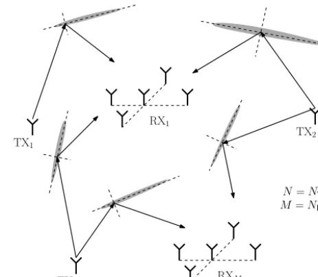
Figure 1. A depiction of a multi-static meteor radar network with multiple transmitters and multiple interferometric receivers. Each transmit–receiver pair observes meteors that match the specular condition, which is usually not met between two different transmit– receiver paths at the same time, and therefore each transmit–receiver path observes an independent set of meteor trails.
An example of a system that uses coded continuous wave constant amplitude radio transmissions is the Global Posi-tioning System (GPS) (Hofmann-Wellenhof et al., 2013). It utilizes phase codes, which are unique for each satellite. This allows each satellite to use the same frequency, which sim-plifies many aspects of calibration and receiver design. This concept of sharing the spectrum between multiple indepen-dent transmit–receive paths is called code division multi-ple access (CDMA) in telecommunications engineering. The similar concept of radar systems with multiple transmitters and multiple receivers is known as multiple-input–multiple-output (MIMO) radar (Haimovich et al., 2008). This term can be applied to a broad range of radar systems with co-located or geographically separated antennas.
In this paper, we provide an overview of the concept of a meteor radar system with multiple transmitters and receivers. We will then go through the signal processing for a radar in-volving multiple transmitters, which is suitable for observ-ing meteor trail echoes. We then show measurements ob-tained during a recent campaign to demonstrate the applica-bility of the method. Finally, we discuss our results, provide an overview of the resulting capabilities, and discuss future plans.
2 Multi-static meteor radar network
de-tected with a monostatic system,NTXis the number of trans-mitter stations,NRXis the number of receiver stations, and c(d) is a factor that depends on the distance (d) between transmitter and receiver. The longer the distance, the smaller this value gets. Typically this factor is between 0.3 and 0.8, which is based on prior bistatic observations (Stober and Chau, 2015). This estimate can be used as a guideline when estimating the number of meteor trails detected with a multi-static meteor radar network.
For example, consider the following network: 5 receiver antenna fields with 5 receiver antennas each, and 10 transmit-ters, each with a single antenna. In this network, there are 35 antennas in total, but it observes approximately the number of meteors that 25 independent monostatic systems would, assuming c(d)=0.5. However, 25 monostatic meteor radar systems would require 150 antennas in total.
3 Signal processing
The key to coded continuous wave radar measurements is deconvolution of echoes from coded transmissions. This can be performed either in the frequency domain or in the time domain. See, e.g., Riad (1986) and references therein. Fre-quency domain methods make use of the well-known prop-erty of Toeplitz matrices that allows them to be represented with a diagonal matrix in the frequency domain (Gray, 1971). Because of this, the maximum likelihood estimator (Eq. 7) can be often expressed with diagonal matrix theory and co-variance matrices and are thus in a numerically efficient computation. At the same time, the frequency domain meth-ods cannot deal with missing measurements or edge effects. Time domain methods are more computationally expensive because a full matrix representation of the theory matrix is needed, even though mathematically in many cases the esti-mator is equivalent to the frequency domain case. However, the time domain representation easily deals with edge effects and missing measurements. The time domain method also al-lows greater flexibility in determining coherence time of the radar target. For the above reasons, we will discuss the the-ory in time domain only. We will also outline a scheme that allows the time domain maximum likelihood estimator to be computed in a numerically efficient manner.
3.1 Coherent deconvolution with linear least squares
Meteor trail echoes are associated with very small Doppler shifts due to the neutral wind. Given a short enough time pe-riod, the complex target scatter coefficient can be assumed to be constant. Even though a single meteor is a point target in range, multiple meteor echoes are often observed simul-taneously. There are also many cases where meteor echoes can spread in range. Therefore, it is beneficial to treat our unknown as a range spread coherent radar target. The coher-ence assumption is made by assuming that the target scatter
as constant overLsamples. We will refer to this as the co-herence time.
In time domain, a radar measurement equation for a radar target that changes amplitude as a function of time is
mt = R
X
r=0
t−rζr,i+ξt, (1)
where mt ∈C is the measured complex baseband voltage seen by the receiver,t ∈Cis the radar transmission wave-form, and ζr,i∈Cis the target backscatter coefficient at a given range gater and coherence timei. Receiver noise is modeled with ξt ∈C. We assume that it is a proper com-plex Gaussian random process ξt∼NC(0, 6), with 6 the
covariance matrix describing the correlation structure of the receiver noise.
In a multi-static measurement with multiple transmitters operating on the same center frequency, there can be multiple different propagation paths that are simultaneously actively probed by a certain receiver. In order to differentiate between transmitters, each transmitter should have a different trans-mit waveformt,k∈C. We use k∈ [0, N] ∈Nto index the transmitters. In this case the measurement equation is a sum of convolutions, with one convolution for each transmitter– receiver pair received by a single station
mt = N
X
k=0
R
X
r=0
t−r,kζr,i,k+ξt, (2)
where also the scatter is different for each transmitter– receiver propagation pathζr,i,k∈C.
Let us first write the inner sum of this equation in matrix form:
mi= N
X
k=0
Ai,kxi,k+ξi, (3)
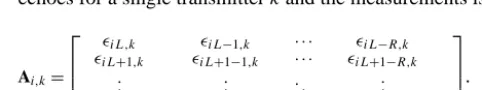
where the unknown parameters – i.e., radar echoes from transmitter k and time t∈ [iL, (i+1)L−1] – are xi,k= [ζ0,i,k,· · ·, ζR,i,k]T ∈CR, and the measurement vector is mi= [miL, miL+1,· · ·, m(i+1)L−1]T ∈CL. Here the theory matrix Ai,k∈CL×R providing the linear relation between echoes for a single transmitterkand the measurements is
Ai,k=
iL,k iL−1,k · · · iL−R,k
iL+1,k iL+1−1,k · · · iL+1−R,k
. .
. ... . .. ...
(i+1)L−1,k (i+1)L−1−1,k · · · (i+1)L−1−R,k
. (4)
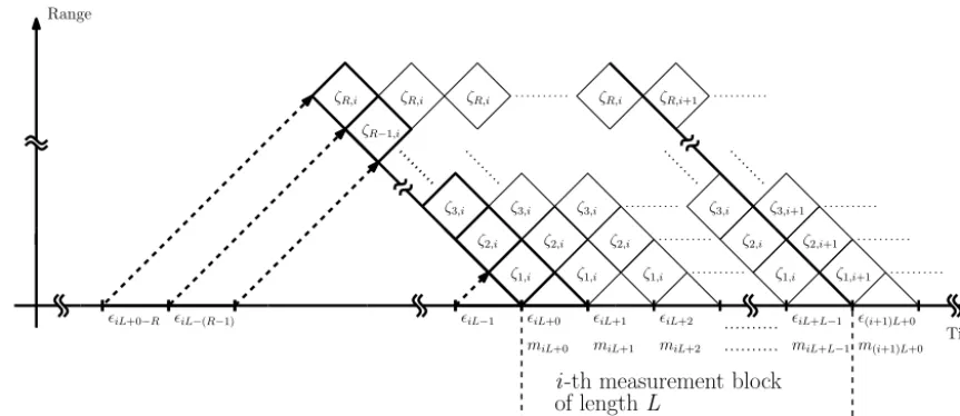
This is depicted in the form of a range–time diagram in Fig. 2.
Equation 3 can be expressed as an equation with just a single matrix
iL+0 iL+2 iL+L−1 ζ1,i ζ1,i ζ1,i ζ1,i+1 ζR,i
ζR,i ζR,i ζR,i+1
(i+1)L+0 Range
Time
i-th measurement block ζ1,i
ζ2,i
ζ2,i ζ2,i
ζ3,i
ζ2,i
ζ3,i+1
ζ2,i+1 ζ3,i
ζ3,i
ζ3,i
ζR,i
iL+0−R iL−(R−1)
miL+0 miL+2 iL+1
miL+1 miL+L−1 m(i+1)L+0 iL−1
of lengthL
ζR−1,i
Figure 2. A range–time diagram describing the relation between coherence time, range gates, and the transmit envelope.
where the theory matrix is a set of stacked convolution ma-trices:
Ai = [Ai,0,· · ·,Ai,N], (6) and the unknown vector is a set of stacked parameter vectors xi= [xTi,0,· · ·,xTi,N]T.
The maximum likelihood estimate for the unknown pa-rameters (i.e., echoes for all the range gates and all transmit– receiver pairs) can be obtained using the standard maximum likelihood formula (Schreier and Scharf, 2010) for complex linear-least-squares problems with proper complex normal random errors:
xi,ML=(A†i6−1Ai)−1A†i6−1mi, (7) which is solvable as long as A†i6−1A
i is not singular. Here † is the Hermitian operation, i.e., a conjugate and transpose. With just a few transmitters using independent pseudoran-dom transmit waveforms, there are more measurements than unknownsL≥N Rand the problem is overdetermined and solvable using Eq. (7).
Code optimality is determined by how good the a posteri-ori covariance matrix is
6post=(A†i6−1Ai)−1. (8)
For a single transmitter–receiver case, Frank and Chu codes (Frank, 1973) are known to be perfect: they result in the smallest possible constant diagonal value of 6post. However, pseudorandom codes are also known to have near-optimal covariance matrix structure (Vierinen et al., 2008). 3.2 Treating other transmissions as noise
If each station utilizes a different pseudorandom trans-mit waveform that is statistically orthogonal from one an-other, i.e., Et,kt∗0,k0=0 for all t and t0 when k6=k0 and
Et,k∗t0,k0 =0 for allkandk0whent6=t0, one can analyze
the multi-static measurements by assuming that there is only one transmitter, and the signals from other transmitters are additive noise
mi=Ai,kxi,k+ξ0i, (9)
where ξ0i=ξi+P
k06=kAi,k0xi,k0. If the radar echoes have
a low signal-to-noise ratio, then we can assume thatξ0i∼ NC(0,6) and that ξ0i≈ξi because the echoes from other transmitters do not significantly contribute to the receiver noise. This allows us to treat each transmit–receive pair as an independent radar measurement. This significantly sim-plifies the estimation problem for large-scale multi-static net-works. In this case, the maximum likelihood estimate for each transmitter–receiver pair is obtained with theory matrix Ai,kused in Eq. (7).
With high signal-to-noise ratio, using the signal propaga-tion path model in Eq. (9) is not as accurate. But even then, the effect of not modeling the echoes from other transmis-sions properly only results in an increase in the variance of the estimates. If the radar transmit waveform is considered as a zero-mean random variable, then the error termξ0is also a zero-mean random process, and the linear-least-squares esti-mator still provides an unbiased estiesti-mator, albeit not the most optimal one.
3.3 Numerically efficient solution
In the previous sections, we did not restrict the waveform in any way, although we mention that pseudorandom wave-forms are good wavewave-forms to use. In practice, from a numer-ical point of view, there are good reasons to design a wave-form in such a way that it repeats after a short enough period of time.
intensive portion of the linear-least-squares estimator: B=(A†6−1A)−1A†6−1. (10)
The maximum likelihood estimate for target backscatter can then be obtained with xML=Bm. If the coherence as-sumptionLis shorter than the length of the repeating pseu-dorandom sequenceLs, the maximum likelihood can still be precalculated, but there have to beLs/Lprecalculated matri-ces Bi∈CN R×Lthat cycle through, assuming that there are an integer number of coherence lengths in the pseudorandom cycle lengthi∈ [1, Ls/L].
With a precalculated maximum likelihood estimation ma-trix, the deconvolution can be performed significantly faster than real time with a modern personal computer. Our de-convolution software is currently implemented with Python script that uses NumPy for computationally intensive por-tions of the code. This software can easily keep up with five receive channels at receive bandwidths of around 100 kHz and 10 µs range gates up to 1500 km.
3.4 Bursty interference
When using the matrix method for analyzing target echoes, it is possible to deal with bursty interference from nearby power-line interference or a nearby radar using short trans-mit pulses. The rows corresponding to bad measurements can be detected using a statistical outlier test and simply removed from the theory matrix and measurement vector. This method works as long as A†6−1A is not singular. This is typically the case if there are more measurements than unknown pa-rameters. Leaving out rows with time localized interference however prevents the use of a precalculated maximum like-lihood estimation matrix, which results in a numerically less efficient solution for the target scatter estimate.
3.5 Target detection
When detecting targets, we assume that each target is point-like and has a Doppler shift. Specular echoes have very small range migration, which means that we can assume them to be at a fixed range gate. The following equation can be used for a model when detecting targets:
ma,t=t−rσ γa(α, φ)eiωt+ξt, (11) where ma,t∈C is the complex baseband voltage received with antenna a∈N, σ∈C the complex scattering coeffi-cient,γa(α, φ)∈Cis the direction of arrival-dependent delay as complex phase with azimuthα∈ [0,2π] ⊂Rand eleva-tionφ∈ [0, π/2] ⊂R, andω∈Ris Doppler shift. The term
ξt ∼NC(0, bI)is measurement noise, which is assumed to be proper complex Gaussian white noise with covariance ma-trixbI. Hereb∈Ris a constant that determines the receiver noise power.
In matrix form this is
m=Aθx+ξ, (12)
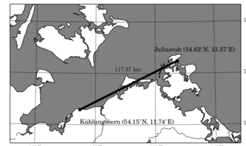
Figure 3. Geometry for the bistatic meteor radar experiment. The transmitter was located in Juliusruh, and the receiver was located at Kühlungsborn, a 118 km great-circle distance from the transmitter.
wheremis a vector of measured complex baseband voltages from all antennas. The moving point target model parameters areθ= [ω, r, α, φ]T. The vector x= [σ]T is a single element vector containing the complex target scatter coefficient.
This is a non-linear statistical inverse problem with a like-lihood density function proportional to
p(m|θ,x)∝expn−kAθx−mk2
o
. (13)
The peak of this distribution (i.e., the maximum likelihood estimator for target parametersθ) is
θML=argmaxθkA †
θmk
2, (14)
which has been shown for moving point targets by, e.g., Markkanen et al. (2005) for space debris. In practice, the maximum likelihood parameters are found using a suffi-ciently dense grid search in parameter space, which in this case includes range, Doppler, and angle of arrival.
4 Juliusruh–Kühlungsborn experiment
In order to test the principle of coded CW meteor radar in practice, we performed a bistatic measurement campaign be-tween 18:00 UTC on 10 June 2015 and 09:00 UTC on 12 June 2015.
In this experiment, the transmitter station was lo-cated in Juliusruh (54◦37017.54800N, 13◦22015.67500E), and the receiver system was located in Kühlungsborn (54◦08048.66500N, 11◦44031.20900E). The locations of the transmitter and receiver are shown in Fig. 3. The same bistatic configuration has been used in Stober and Chau (2015).
4.1 Measurement setup
which results in a 1.5 km range resolution. Due to the rep-etition of the code after 1000 bits, the range aliasing of this experiment occurs at 3000 km. Note that this is not an inher-ent limitation of the method. In order to increase this aliasing range, a longer code can be used. The code was sent continu-ously in a repeated fashion to allow the use of a numerically efficient precalculated maximum likelihood estimation ma-trices in the analysis as described in Sect. 3.3.
The transmitted waveform was generated with a PC, with Gaussian pulse shaping performed with a FIR filter. The digi-tal transmit waveform is then transferred over a 1 Gb Ethernet connection to a USRP-N200 software-defined radio, which converts the digital baseband signal to an analog signal cen-tered at 32.55 MHz with a 100 kHz bandwidth. The USRP N200 was synchronized to the global reference clock using a Trimble Thunderbolt GPS disciplined oscillator (GPSDO). The signal generated by the USRP N200 was then amplified to 30 W of continuous power and fed through a low-pass fil-ter to suppress harmonic emissions. The 30 W signal was fed to the three-element Yagi transmit antenna of the Juliusruh SKiYMET meteor radar. Only one linear polarization com-ponent was used.
In Kühlungsborn, the signals were received with five Yagi antennas arranged in a so-called Jones configuration (Jones et al., 1998). These are the same antennas that are used routinely as a bistatic receiver for the Juliusruh pulsed SKiYMET meteor radar. The receiving antennas were con-figured to receive circular polarization. The five-channels were recorded using a five channel USRP N200 receiver setup, which was synchronized to a global reference using a Trimble Thunderbolt GPSDO. The receivers were synchro-nized to one another using a 1 PPS and 10 MHz signal from the GPSDO. The five channels were recorded at a 1 MHz bandwidth and further FIR filtered and decimated to 100 kHz using a Gaussian pulse shaping filter to reduce out-of-band emissions. The signals were recorded to an external hard drive for offline processing.
4.2 Results
In order to ascertain the performance of our low-power coded CW meteor radar concept, we compare the results from our bistatic campaign with existing SKiYMET operational pulsed specular meteor radar (SMR) measurements. First, we compare the distributions of some selected parameters ob-tained during 24 h of operations between our CW and a stan-dard pulsed experiment, operating on the same multi-static configuration operating in the same bistatic configuration. Since the same antennas were used, a simultaneous compar-ison is not possible. However, as we show below, the com-parisons are meaningful. Second, we compare the winds ob-tained with the coded CW measurements with those obob-tained from the monostatic SMR system located in Collm (Jacobi, 2006),∼350 km south of our Juliusruh–Kühlungsborn ob-servations.
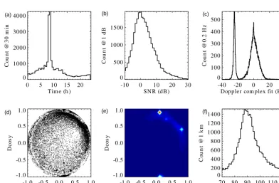
In Fig. 4, we show selected results of the CW experiment conducted on 11 June 2015: (a) meteor count as a function of time of the day, (b) signal-to-noise (SNR) distributions, (c) Doppler velocity distribution, (d) echo location, (e) bivariate distribution of the precedence of echoes, as function of di-rection cosines inx(west to east) andy (south to north) di-rections; and (e) altitude distribution. These parameters have been obtained on the detected echoes, which were detected with the detection schemes described in Sect. 3.5. After de-tection, the parameter estimation has been done followed by the procedures similar to those described in Hocking et al. (2001) and Holdsworth et al. (2004). We show the results of all the possible meteor-like echoes detected above 140 km to-tal range (i.e., 70 km for a round-trip monostatic range), since range-aliased meteor echoes are not expected in this coded CW experiment.
The results obtained a few days earlier (4 June 2015) with a pulsed SMR, using the same bistatic configuration, are shown in Figs. 5 and 6. These measurements have been obtained with a 15 kW peak power transmitter, 625 Hz pulse repetition frequency (i.e., maximum total unambigu-ous range of 480 km), and 10 µs sampling. The results are obtained using the same identification procedure used with the CW data, while the detection is the standard detection used in our operational pulsed-Doppler systems. In Fig. 5, we show the results of all meteor-like echoes before clean-ing. The results after a cleaning procedure including the se-lection of echoes with underdense characteristics are shown in Fig. 6. The cleaning procedure consists mainly in remov-ing those echoes that do not present clear underdense char-acteristics (Holdsworth et al., 2004), or are outside the ex-pected altitude range between 70 and 120 km. Most of the echoes that have been removed are caused either by pulsed external radio interference, non-specular meteor echoes, and airplane echoes. Note that specular meteor echoes coming from ranges above 480 km will be range-aliased into lower ranges, where ground and airplane echoes occur.
By comparing Figs. 5 and 6, we can clearly see that many non-meteor echoes were originally detected. They are clearly visible as narrow distributions in all the plots, but more pro-nounced in the bivariate direction cosine distributions (i.e., coming from specific locations) and in the velocity distri-butions (showing larger Doppler shifts than expected). The origin for these echoes is most likely man-made radio inter-ference.
0 5 10 15 20 Time (h) 0 50 100 150 200 250 C ou n t @ 3 0 m in
-10 0 10 20 30
SNR (dB) 0 200 400 600 800 C ou n t @ 1 d B
-40 -20 0 20 40
Doppler complex fit (Hz) 0 20 40 60 80 100 120 140 C ou n t @ 0 .2 H z
-1.0 -0.5 0.0 0.5 1.0 Dcosx -1.0 -0.5 0.0 0.5 1.0 D cos y
-1.0 -0.5 0.0 0.5 1.0 Dcosx -1.0 -0.5 0.0 0.5 1.0 D cos y
70 80 90 100 110 120 Height (km) 0 100 200 300 400 C ou n t @ 1 k m
Number of detections 04691 11-J un-2015 (162)
(a) (b) (c)
(d) (e) (f)
Figure 4. Summary results from coded CW specular meteor radar experiment for 24 h taken on 11 June 2015. (a) Count as function of day, (b) SNR histogram, (c) Doppler velocity histogram, (d) echo location, (e) echo location bivariate histogram, and (f) altitude distribution.
(a) (b) (c)
(d) (e) (f)
0 5 10 15 20 Time (h) 0 1000 2000 3000 4000 C ou n t @ 3 0 m in
-10 0 10 20 30 SNR (dB) 0 500 1000 1500 C ou n t @ 1 d B
-40 -20 0 20 40 Doppler complex fit (Hz) 0 100 200 300 400 500 C ou n t @ 0 .2 H z
-1.0 -0.5 0.0 0.5 1.0 Dcosx -1.0 -0.5 0.0 0.5 1.0 D cos y
-1.0 -0.5 0.0 0.5 1.0 Dcosx -1.0 -0.5 0.0 0.5 1.0 D cos y
70 80 90 100 110 120 Height (km) 0 200 400 600 800 1000 1200 1400 C ou n t @ 1 k m
Number of detections 29286 4-J un-2015 (155)
(a) (b) (c)
(d) (e) (f)
0 5 10 15 20 Time (h) 0
50 100 150 200
C
ou
n
t
@
3
0
m
in
-10 0 10 20 30 SNR (dB) 0
100 200 300 400
C
ou
n
t
@
1
d
B
-40 -20 0 20 40 Doppler complex fit (Hz) 0
20 40 60 80 100 120
C
ou
n
t
@
0
.2
H
z
-1.0 -0.5 0.0 0.5 1.0 Dcosx
-1.0 -0.5 0.0 0.5 1.0
D
cos
y
-1.0 -0.5 0.0 0.5 1.0 Dcosx
-1.0 -0.5 0.0 0.5 1.0
D
cos
y
70 80 90 100 110 120 Height (km) 0
100 200 300 400
C
ou
n
t
@
1
k
m
Number of detections 05894 4-J un-2015 (155)
Figure 6. Same as Fig. 5, but with false detections that are considered to be caused by external interference are removed, in addition to echoes that are considered to be from overdense meteor trails.
Instead we observe that with the detection procedures used, specular meteor echoes are detected when SNRs are greater than∼0 and∼ −6 dB in the CW and pulsed systems, respec-tively. A fairer comparison would have been to use the same detection procedures in both data sets (e.g., using the Doppler grid search used in the CW experiment also in the pulse sys-tem). However, we have preferred to compare existing proce-dures in a standard pulsed-system, against the improvements in both transmission as well as in signal processing in the proposed coded CW system.
To further demonstrate the quality of our coded CW sys-tem results, in Fig. 7 we present the derived winds obtained with the CW experiment: zonal and meridional (bottom) wind. The winds are derived using the approach outlined in Hocking et al. (2001), Holdsworth et al. (2004), and Stober et al. (2012), i.e., assuming a horizontal homogeneity of the horizontal wind in the observed volume. The resulting winds show typical summer conditions for a northern mid-altitude station with the expected wind reversal at around 90 km alti-tude in the zonal flow. Further, both wind components show a strong semidiurnal oscillation.
The winds observed during the same time with the Collm system are shown in Fig. 8. As there is no direct overlap between both observation volumes, a one-to-one correspon-dence of the measured zonal and meridional winds is not ex-pected. However, the main general features observed with the CW system are also observed with the Collm system.
Figure 7. Zonal and meridional wind derived from the CW exper-iment using the forward scatter radio link between Juliusruh and Kühlungsborn.
5 Discussion
deconvo-Figure 8. Zonal and meridional wind as observed by the Collm me-teor radar approximately 350 km south of the CW radio link be-tween Juliusruh and Kühlungsborn.
lution of coherent echoes assuming zero Doppler shift does not work, as the assumption of constant phase and amplitude of backscatter during a pulse compression period is not valid. This issue starts to become significant when the phase of the echo rotates more than 10 % of 2πdue to Doppler (≈50 Hz Doppler shift for our setup). However, these cases could be analyzed with two other approaches: a filter matched in Doppler and range (Markkanen et al., 2005), or using a sparse model of the target in range–Doppler space (Volz and Close, 2012). Pseudorandom phase coded continuous radar transmit waveforms are well suited for both of these analysis methods. Therefore, bulk Doppler shifts that are seen with meteor head echoes can also be observed with coded CW radars.
Small coherent scatter radars (including SMRs) can also observe echoes from non-specular meteor echoes, E-region field-aligned irregularities (Hysell et al., 2004; Hysell and Chau, 2001), or other interesting phenomena such as the me-teor radar observations of the failed Russian missile experi-ment (Kozlovsky et al., 2014). Non-specular meteor echoes could also be due to field-aligned irregularities or charged dust (Chau et al., 2014). Some of these echoes can have a large range and Doppler spread, which often makes their analysis problematic with pulsed radars with high pulse rep-etition rate measurements, which are designed for a point tar-get at altitudes between 70 and 120 km. A coded CW trans-mit waveform would be more suitable for these types of mea-surements of opportunity, without the range–Doppler ambi-guity. With coded CW, even highly overspread targets can be analyzed using lag-profile inversion (Virtanen et al., 2008). Pseudorandom phase coded waveforms are known to be suit-able for lag-profile inversion (Sulzer, 1986; Vierinen et al., 2008), allowing the full range of Doppler frequencies
mea-sured by the receiver (in the case of 100 kHz receiver band-width±50 kHz) to be analyzed if necessary.
One downside for coded continuous wave meteor radar is that there has to be sufficient separation between the trans-mitter and receivers to avoid saturation of the receivers. While we used a distance of 118 km in our test, the distance between the transmitter and receiver could be significantly smaller, which would result in a measurement closer to that of a monostatic SMR. We have not determined the minimum distance needed to avoid saturation for typical meteor radar receiving antennas, but we have in the past demonstrated that a 20 W coded continuous high-frequency radar with trans-mitter and receiver is separated by 500 m. This suggests that a separation of a few kilometers is feasible also with a con-tinuously transmitting meteor radar.
Another factor that affects bistatic meteor radar receivers is that they tend to detect more meteors at lower elevations than a monostatic radar. This can be seen in the measure-ments shown in Fig. 4. Lower-elevation detections are known to have larger errors in true height determination (Hocking, 2004), which degrades the quality of the data products. This has to be addressed, e.g., by using an interferometer configu-ration that is better suited for elevation detections or by using short transmit–receive paths.
6 Conclusion
We have described the concept of a continuously transmitting pseudorandom phase coded specular meteor radar. The main advantages of the system are the following: (a) it can oper-ate with lower peak power than a pulsed system with similar average power, (b) it is suitable for a large-scale multi-static radar network, (c) it does not suffer from the range–Doppler ambiguity problem, (d) there is no inherent limit to time res-olution, and (e) it is less susceptible to false detections due to radio interference when compared with pulsed systems. The latter is possible since the pulse-like interferences would be spread in range and Doppler in the decoding process.
We would like to stress the suitability of the presented type of radar for a large-scale multi-static radar network. Not only would the low-power transmitting systems with coded wave forms be more friendly with other radio users in nearby bands, but also the receiving systems could be simplified, by allowing the reception of multiple transmitters on the same antenna and same frequency. The separation of the different transmitted signals would be done by knowing the code of each transmitter site. The only restriction is that the transmit-ter cannot be extremely close to the receiver, to avoid satura-tion of the receiver amplifier.
in-teference (RFI), which is apparent from Figs. 4, 5, and 6, which compare detections with the coded CW bistatic mea-surements and the pulsed bistatic meamea-surements obtained us-ing the same geometry and antennas. We expect that better results, i.e., more meteor counts, could be easily obtained by increasing the transmitter power from 30 W, or by adding more transmitters and receivers to measure the same volume. The zonal and meridional winds derived with the coded bistatic CW meteor trail measurements agree well with the Collm monostatic pulsed meteor radar system, which indi-cates that the data quality is of sufficient quality to be used for mesosphere–lower-thermosphere (MLT) wind determina-tion. Further exploring the concept with a larger number of transmitters and receivers is a topic of future work.
Even though we have focused on the use of the coded CW method for specular meteor radars in this study, we have al-ready applied the same signal processing principles for verti-cal high-frequency radar and ionosonde measurements. This type of a radar transmission principle would work well also with, e.g., the SuperDARN type of a high-frequency over-the-horizon radar. Discussing these applications is a topic of future work. In these applications, the benefits of the method are similar: reduction of peak transmit power, removal of range–Doppler ambiguity, more tolerance to interference, more flexibility in spectral resolution, and the possibility of sounding multiple channels with the same frequency simul-taneously.
Acknowledgements. The authors would like to thank Dieter Keuer, Jens Mielich, and Jörg Trautner for help with performing the measurements in Juliusruh and Kühlungsborn. We thank Christoph Jacobi for supporting the Collm meteor radar obser-vations. We would also like to thank the anonymous referees for valuable assistance in improving the quality of this paper.
Edited by: M. Nicolls
References
Appleton, E. and Naismith, R.: The radio detection of meteor trails and allied phenomena, P. Phys. Soc., 59, 461–473, 1947. Appleton, E. V. and Barnett, M. A.: Local reflection of wireless
waves from the upper atmosphere, Nature, 115, 333–334, 1925. Breit, G. and Tuve, M. A.: A test of the existence of the
conduct-ing layer, Phys. Rev., 28, 554–575, doi:10.1103/PhysRev.28.554, 1926.
Chau, J., Strelnikova, I., Schult, C., Oppenheim, M., Kelley, M., Stober, G., and Singer, W.: Nonspecular meteor trails from non-field-aligned irregularities: Can they be explained by presence of charged meteor dust?, Geophys. Res. Lett., 41, 3336–3343, 2014. Dyrud, L. P., Oppenheim, M. M., Close, S., and Hunt, S.: Interpre-tation of non-specular radar meteor trails, Geophys. Res. Lett., 29, 8-1–8-4, 2002.
Elford, W. and Robertson, D.: Measurements of winds in the upper atmosphere by means of drifting meteor trails II, J. Atmos. Terr. Phys., 4, 271–284, 1953.
Evans, J.: Radar observations of meteor deceleration, J. Geophys. Res., 71, 171–188, 1966.
Evans, J. V. and Hagfors, T.: Radar astronomy, edited by: Evans, J. V., Hagfors, Tor, 1, McGraw-Hill, New York, 1968.
Frank, R.: Comments on “Polyphase codes with good periodic cor-relation properties” by Chu, David C., IEEE T. Inform. Theory, 19, 244–244, 1973.
Gray, R. M.: Toeplitz and circulant matrices: A review, vol. 1, Infor-mation Systems Laboratory, Stanford Electronics Laboratories, Stanford University, Stanford, 1971.
Greenhow, J. and Hall, J.: The height variation of the ambipolar diffusion coefficient for meteor trails, Planet. Space Sci., 5, 109– 114, 1961.
Haimovich, A. M., Blum, R. S., and Cimini, L. J.: MIMO radar with widely separated antennas, IEEE Signal Proc. Mag., 25, 116– 129, 2008.
Herlofson, N.: The theory of meteor ionization, Rep. Prog. Phys, 11, 444–454, doi:10.1088/0034-4885/11/1/313, 1947.
Hey, J., Parsons, S., and Stewart, G.: Radar observations of the Gi-acobinid meteor shower, 1946, Mon. Not. R. Astron. Soc., 107, 176–183, 1947.
Hocking, W., Fuller, B., and Vandepeer, B.: Real-time determina-tion of meteor-related parameters utilizing modern digital tech-nology, J. Atmos. Sol.-Terr. Phy., 63, 155–169, 2001.
Hocking, W. K.: Temperatures Using radar-meteor
de-cay times, Geophys. Res. Lett., 21, 3297–3300,
doi:10.1029/1999GL003618, 1999.
Hocking, W. K.: Radar meteor decay rate variability and at-mospheric consequences, Ann. Geophys., 22, 3805–3814, doi:10.5194/angeo-22-3805-2004, 2004.
Hofmann-Wellenhof, B., Lichtenegger, H., and Collins, J.: Global positioning system: theory and practice, Springer Science & Business Media, Wien, 2013.
Holdsworth, D. A., Reid, I. M., and Cervera, M. A.: Buckland Park all-sky interferometric meteor radar, Radio Sci., 39, RS5009, doi:10.1029/2003RS003014, 2004.
Hysell, D. L. and Chau, J. L.: Inferring E region electron density profiles at Jicamarca from Faraday rotation of coherent scatter, J. Geophys. Res., 106, 30371–30380, 2001.
Hysell, D. L., Larsen, M. F., and Zhou, Q. H.: Common volume co-herent and incoco-herent scatter radar observations of mid-latitude sporadic E-layers and QP echoes, Ann. Geophys., 22, 3277– 3290, doi:10.5194/angeo-22-3277-2004, 2004.
Jacobi, C. A. D. K.: Long-period upper mesosphere temperature and plasma scale height variations derived from VHF meteor radar and LF absolute reflection height measurements, Adv. Ra-dio Sci., 4, 351–355, 2006.
Janches, D., Hocking, W., Pifko, S., Hormaechea, J., Fritts, D., Brunini, C., Michell, R., and Samara, M.: Interferometric me-teor head echo observations using the Southern Argentina Agile Meteor Radar, J. Geophys. Res.-Space, 119, 2269–2287, 2014. Jones, J.: On the decay of underdense radio meteor echoes, Mon.
Not. R. Astron. Soc., 173, 637–647, 1975.
Jones, J., Brown, P., Ellis, K., Webster, A., Campbell-Brown, M., Krzemenski, Z., and Weryk, R.: The Canadian Meteor Orbit Radar: system overview and preliminary results, Planetary Space Sci., 53, 413–421, doi:10.1016/j.pss.2004.11.002, 2005. Kozlovsky, A., Shalimov, S., Lukianova, R., and Lester, M.:
Iono-spheric effects of the missile destruction on 9 December 2009, J. Geophys. Res.-Space, 119, 3873–3882, 2014.
Manning, L., Villard Jr., O., and Peterson, A.: Meteoric echo study of upper atmosphere winds, Proceedings of the IRE, 38, 877– 883, 1950.
Manning, L. A.: The theory of the radio detection of meteors, J. Appl. Phys., 19, 689–699, 1948.
Markkanen, J., Lehtinen, M., and Landgraf, M.: Real-time space de-bris monitoring with EISCAT, Adv. Space Res., 35, 1197–1209, 2005.
Mathews, J.: Radio science issues surrounding HF/VHF/UHF radar meteor studies, J. Atmos. Sol.-Terr. Phy., 66, 285–299, 2004. McKinley, D. W. R.: Meteor science and engineering,
McGraw-Hill, New York, 1, 1961.
Millman, P.: The Radar Meteor Echo (survey Paper), in: Physics and Dynamics of Meteors, vol. 33, p. 3, 1968.
Nagaoka, H.: Possibility of disturbance of radio transmissions by meteoric showers, in: Proc. Imperial Acad. Tokyo, vol. 5, p. 233, 1929.
Oppenheim, M. M., vom Endt, A. F., and Dyrud, L. P.: Electrody-namics of meteor trail evolution in the equatorial E-region iono-sphere, Geophys. Res. Lett., 27, 3173–3176, 2000.
Ostro, S. J.: Planetary radar astronomy, Rev. Mod. Phys., 65, 1235, doi:10.1029/RG021i002p00186, 1993.
Pellinen-Wannberg, A. and Wannberg, G.: Meteor observations with the European incoherent scatter UHF radar, J. Geophys. Res.-Space, 99, 11379–11390, 1994.
Pierce, J. A.: Abnormal ionization in the E region of the ionosphere, P. Ire., 26, 892–908, 1938.
Riad, S. M.: The deconvolution problem: An overview, P. IEEE, 74, 82–85, 1986.
Robertson, D., Liddy, D., and Elford, W.: Measurements of winds in the upper atmosphere by means of drifting meteor trails I, J. Atmos. Terr. Phys., 4, 255–270, 1953.
Sahr, J. D. and Lind, F. D.: The Manastash Ridge radar: A passive bistatic radar for upper atmospheric radio science, Radio Sci., 32, 2345–2358, 1997.
Schreier, P. J. and Scharf, L. L.: Statistical signal processing of complex-valued data: the theory of improper and noncircular sig-nals, Cambridge University Press, Cambridge, 2010.
Stober, G. and Chau, J. L.: A multistatic and multifrequency novel approach for specular meteor radars to improve wind measurements in the MLT region, Radio Sci., 50, 431–442, doi:10.1002/2014RS005591, 2015.
Stober, G., Jacobi, C., Matthias, V., Hoffmann, P., and Gerd-ing, M.: Neutral air density variations during strong plane-tary wave activity in the mesopause region derived from me-teor radar observations, J. Atmos. Sol.-Terr. Phy., 74, 55–63, doi:10.1016/j.jastp.2011.10.007, 2012.
Sugar, G. R.: Radio propagation by reflection from meteor trails, P. IEEE, 52, 116–136, 1964.
Sulzer, M. P.: A radar technique for high range resolution incoher-ent scatter autocorrelation function measuremincoher-ents utilizing the full average power of klystron radars, Radio Sci., 21, 1033–1040, 1986.
Tsutsumi, M., Tsuda, T., Nakamura, T., and Fukao, S.: Tempera-ture fluctuations near the mesopause inferred from meteor ob-servations with the middle and upper atmosphere radar, Radio Science, 29, 599–610, 1994.
Vierinen, J., Lehtinen, M. S., Orispaa, M., and Virtanen, I. I.: Trans-mission code optimization method for incoherent scatter radar, arXiv preprint arXiv:0801.1343, 2008.
Virtanen, I. I., Lehtinen, M. S., Nygrén, T., Orispää, M., and Vieri-nen, J.: Lag profile inversion method for EISCAT data analysis, Ann. Geophys., 26, 571–581, doi:10.5194/angeo-26-571-2008, 2008.
Volz, R. and Close, S.: Inverse filtering of radar signals using com-pressed sensing with application to meteors, Radio Sci., 47, 2012.
Williams, I. P.: The velocity of meteoroids: a historical review, Atmos. Chem. Phys., 4, 471–475, doi:10.5194/acp-4-471-2004, 2004.