www.ocean-sci.net/8/567/2012/ doi:10.5194/os-8-567-2012
© Author(s) 2012. CC Attribution 3.0 License.
Ocean Science
In situ determination of the remote sensing reflectance:
an inter-comparison
G. Zibordi1, K. Ruddick2, I. Ansko3, G. Moore4, S. Kratzer5, J. Icely6, and A. Reinart3 1Institute for Environment and Sustainability, Joint Research Centre, Ispra, Italy
2Royal Belgian Institute of Natural Sciences, Management Unit of the North Sea Mathematical Models, Brussels, Belgium 3Tartu Observatory, Estonia
4Bio-Optika, Crofters, Middle Dimson, Gunnislake, UK
5Stockholm University, Department of Systems Ecology, Sweden 6Sagremarisco Lda, Vila do Bispo, Portugal
Correspondence to: G. Zibordi ([email protected])
Received: 15 February 2012 – Published in Ocean Sci. Discuss.: 7 March 2012 Revised: 15 June 2012 – Accepted: 4 July 2012 – Published: 6 August 2012
Abstract. Inter-comparison of data products from simulta-neous measurements performed with independent systems and methods is a viable approach to assess the consis-tency of data and additionally to investigate uncertainties. Within such a context the inter-comparison called Assess-ment of In Situ Radiometric Capabilities for Coastal Wa-ter Remote Sensing Applications (ARC) was carried out at the Acqua Alta Oceanographic Tower in the northern Adri-atic Sea to explore the accuracy of in situ data products from various in- and above-water optical systems and meth-ods. Measurements were performed under almost ideal con-ditions, including a stable deployment platform, clear sky, relatively low sun zenith angles and moderately low sea state. Additionally, all optical sensors involved in the ex-periment were inter-calibrated through absolute radiometric calibration performed with the same standards and meth-ods. Inter-compared data products include spectral water-leaving radianceLw(λ), above-water downward irradiance Ed(0+,λ)and remote sensing reflectanceRrs(λ). Data prod-ucts from the various measurement systems/methods were directly compared to those from a single reference sys-tem/method. Results forRrs(λ)indicate spectrally averaged values of relative differences comprised between −1 and +6 %, while spectrally averaged values of absolute differ-ences vary from approximately 6 % for the above-water sys-tems/methods to 9 % for buoy-based syssys-tems/methods. The agreement between Rrs(λ) spectral relative differences and estimates of combined uncertainties of the inter-compared systems/methods is noteworthy.
1 Introduction
Climate studies largely rely on environmental indices de-rived from remote sensing data (e.g. Behrenfeld et al., 2006; Achard et al., 2002; Kaufman and Tanr´e, 2002; Stroeve et al., 2007). Satellite ocean color data are also increasingly applied for coastal and inland water management, includ-ing water quality monitorinclud-ing, harmful algal bloom detection and sediment transport studies (Brando and Dekker, 2003; Stumpf and Tomlinson, 2005; Ruddick et al., 2008). How-ever, the confident use of these data requires the quantifi-cation of their uncertainties. This is generally accomplished through the comparison of satellite products with in situ ref-erence measurements. In the case of satellite ocean color, the spectral remote sensing reflectanceRrsdetermined from top-of-atmosphere radiance is the primary data product used for the generation of higher level products such as chlorophylla
concentration (Chla). As a consequence, access to accurate in situ Rrs is essential for the assessment of primary data products from satellite ocean color missions.
lead to unpredictable uncertainties affecting the assessment of satellite products.
The quantification and the successive reduction of uncer-tainties for in situ measurements is thus a major challenge for ocean color scientists actively involved in field radiome-try. Basic tasks include the precise implementation and ap-plication of established measurement and analysis methods, and additionally an investigation and quantification of each source of uncertainty in primary data products. Best practice suggests the verification of each measurement and process-ing step through inter-comparison exercises.
This work summarizes results from a radiometric inter-comparison performed in the northern Adriatic Sea with the main objective of evaluating the agreement of in situ Rrs products determined through the application of independent measurement systems and methods.
2 The inter-comparison
Inter-comparison activities are essential to evaluate the per-formance of independent measurement methods and also the ability of individuals to properly implement them (e.g. Thome et al., 1998; Hooker et al., 2002a; Barton et al., 2004). A major requirement for field inter-comparisons is the need for performing measurements with different sys-tems/methods under almost identical conditions. In the case of optical oceanography, this is better achieved with the use of fixed deployment platforms instead of ships. In fact, grounded platforms offer the major advantage of deploying instruments under controlled geometries not affected by su-perstructure drift and roll. This favourable situation is easily achieved at the Acqua Alta Oceanographic Tower (AAOT) in the northern Adriatic Sea (e.g. Zibordi et al., 1999, 2009a; Hooker and Zibordi, 2005).
The inter-comparison activity presented and discussed in this work focuses on a variety of measurement systems and methods applied to produce in situ data for the validation of marine primary radiometric products for the Medium Reso-lution Imaging Spectrometer (MERIS) onboard the Envisat platform of the European Space Agency (ESA). The inter-comparison, called Assessment of In Situ Radiometric Ca-pabilities for Coastal Water Remote Sensing Applications (ARC) was conceived within the framework of the MERIS Validation Team (MVT) and supported by ESA in the context of international activities promoted by the Working Group on Calibration and Validation (WGCV), Infrared and Visi-ble Optical Systems (IVOS) subgroup of the Committee on Earth Observation Satellites (CEOS).
ARC activities comprise two successive phases carried out during July 2010. In the first phase, field measurements were carried out at the AAOT during four days character-ized by favourable illumination and sea state conditions. In the second phase, the optical sensors previously deployed at the AAOT were inter-calibrated at the Joint Research Centre
(JRC). This inter-calibration was achieved through the abso-lute radiometric calibration of the optical sensors by using identical laboratory standards and methods, with the excep-tion of one system (see Sect. 3.3.3) also calibrated at the JRC using the same standards and methods, but at a different time. Data products included in the inter-comparison were then all computed from data calibrated (or corrected) using consis-tently determined radiometric coefficients.
The inter-comparison of data products from different mea-surement systems and methods is here performed, relying on data from a single system/method considered as the refer-ence because of its well documented performances and long-standing application to the validation of satellite ocean color products. Due to the variety of multispectral and hyperspec-tral sensors included in the inter-comparison, the data anal-ysis has been restricted to the center-wavelengths of major interest for satellite ocean color: 412, 443, 490, 510, 555, and 665 nm. The presentation of results is supported by un-certainty budgets quantified for each system/method.
3 Measurement systems and methods
The ARC inter-comparison includes an assortment of in- and above-water measuring systems and methods. To rational-ize their description, the basic elements common to generic methods (i.e. in- and above-water) are hereafter summarized, then details on each measurement system and method are provided. It is anticipated that the analysis of results is fo-cused on Rrs determined according to its simplest defini-tion (see Sect. 3.1) without applying any correcdefini-tion for the anisotropy of in-water radiance distribution (i.e. the bidirec-tional effects). In fact, the objective of this work is to quan-tify differences among fundamental radiometric products de-rived from the application of various systems and methods; the use of the same scheme to account for bidirectional ef-fects would not impact the comparison, while the application of different schemes is out of the scope of the study. In line with such a strategy, the dependence on the viewing geome-try of above-water measurements (also depending on the in-water radiance distribution) has been addressed by applying an identical correction scheme for all considered methods. 3.1 Overview on in-water measurements
changes on in-water radiometric measurements during data collection.
In-water continuous profiles of radiometric quantities re-sult generally from measurements performed with optical sensors operated on profiling systems (e.g. winched or free-fall). Due to wave focusing and defocusing, the accuracy of sub-surface radiometric products largely depends on the sam-pling depth interval and on the depth resolution (Zaneveld et al., 2001; D’Alimonte et al., 2010). Thus, highly accurate in-water radiometric products can only be determined by sam-pling near the surface (especially in coastal regions due to possible vertical non-homogeneities in the optical properties of seawater), and by producing a large number of measure-ments per unit depth not significantly affected by tilt (Zibordi et al., 2004a).
In-water fixed-depth profiles mostly result from the use of optical sensors operated on buoys at nominal depths. These buoy-based systems generally provide the capability of mea-suringLu(z, λ, t),Ed(z, λ, t) and possibly alsoEu(z, λ, t) at multiple depths (typically between 1 and 10 m), in addition to
Ed(0+,λ, t). By neglecting the effects of system tilt, the ac-curacy of radiometric products determined with buoy-based systems is a function of the discrete depths selected for the optical sensors, the acquisition rate and the duration of log-ging intervals (Zibordi et al., 2009a).
The same data reduction process is in principle applicable to both fixed-depth and continuous profile radiometric data =(z, λ, t )(i.e.Lu(z, λ, t),Eu(z, λ, t) andEd(z,λ,t )). The ini-tial step, leading to minimization of perturbations created by illumination change during data collection, is performed ac-cording to:
=0(z, λ, t0)=
=(z, λ, t ) Ed(0+, λ, t )
Ed(0+, λ, t0), (1)
where =0(z, λ, t0) indicates radiometric values as if they were all taken at the same timet0, and Ed(0+, λ, t0) speci-fies the above-water downward irradiance at timet0(witht0 generally chosen to coincide with the beginning of the acqui-sition sequence).
Omitting the variable t, the sub-surface quantities =0(0−, λ)(i.e.Lu(0−, λ),Eu(0−, λ)andEd(0−, λ))are then determined as the exponentials of the intercepts resulting from the least-squares linear regressions of ln=0(z, λ)versus
zwithin the extrapolation interval identified byz1< z < z2 and chosen to satisfy the requirement of linear decay of ln=0(z, λ)with depth. The negative values of the slopes of the regression fits are the so-called diffuse attenuation co-efficients K=(λ) (i.e. Kl(λ),Ku(λ) andKd(λ) determined from Lu(z, λ, t), Eu(z, λ, t) and Ed(z, λ, t ) values, respec-tively, from the selected extrapolation interval).
The radiometric quantity of major relevance here is the so-called water-leaving radiance Lw(λ) in units of mW cm−2µm−1sr−1. This is the radiance leaving the sea
quantified just above the surface from:
Lw(λ)=0.543Lu(0−, λ), (2)
where the factor 0.543, derived assuming the seawater re-fractive index is independent of wavelength (Austin, 1974), accounts for the reduction in radiance from below to above the water surface.
A second radiometric quantity central to this study is the remote sensing reflectanceRrs(λ) in units of sr−1, given by: Rrs(λ)=
Lw(λ) Ed(0+, λ)
, (3)
withEd(0+, λ) in units of mW cm−2µm−1.
Rrs(λ)is thus a quantity corrected for illumination condi-tions depending on sun zenith angle, Sun–Earth distance and atmospheric transmittance (Mueller et al., 2002).
3.2 Overview on above-water measurements
Above-water methods generally rely on measurements of (i) total radiance from above the sea LT(θ, 1φ, λ) (that includes water-leaving radiance as well as sky- and sun-glint contributions); (ii) the sky radianceLi(θ0, 1φ, λ); and (iii) usually also Ed(0+, λ). The measurement geometry is defined by the sea-viewing angleθ, the sky-viewing angle
θ0 and the difference between sun and sensor azimuth an-gles,1φ=φ0−φ (Deschamps et al., 2004; Hooker et al., 2004; Zibordi et al., 2004b). The accurate determination of
Lw(λ) then depends on the capability of minimizing glint contributions through the use of suitable measurement ge-ometries (Mobley, 1999), and additionally, the application of statistical filtering schemes toLT(Hooker et al., 2002a; Zi-bordi et al., 2002b), or physically-based correction methods relying on known reflectance properties of seawater in the near-infrared spectral region (Ruddick et al., 2006), or al-ternatively, polarisers to directly reduce sky- and sun-glint (Fougnie et al., 1999).
In the case of non-polarized systems, measurements of
LT(θ, 1φ, λ) and Li(θ0, 1φ, λ) for the determination of
Lw(λ) are generally performed at θ=40◦ and θ0=140◦, with1φchosen between+90◦ and+135◦ or alternatively −90◦and−135◦. The value of1φ= ±135◦ is considered the most appropriate (see Mobley, 1999). However, its ap-plication must be regarded with special care because it may more likely lead to measurements significantly affected by the shadow cast by the deployment superstructure in the anti-solar region (i.e. nearby the sea area seen by the sensor).
The water-leaving radianceLw(θ, 1φ, λ) for a given view-ing geometry is computed as:
Lw(θ, 1φ, λ)=LT(θ, 1φ, λ)
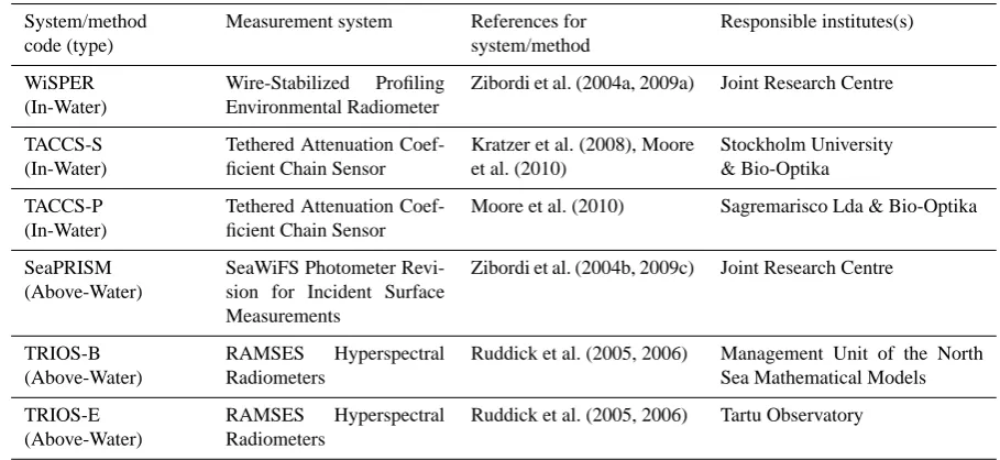
Table 1. Summary of codes assigned to measurement systems/methods together with relevant references and responsible institutes.
System/method code (type)
Measurement system References for system/method
Responsible institutes(s)
WiSPER (In-Water)
Wire-Stabilized Profiling Environmental Radiometer
Zibordi et al. (2004a, 2009a) Joint Research Centre
TACCS-S (In-Water)
Tethered Attenuation Coef-ficient Chain Sensor
Kratzer et al. (2008), Moore et al. (2010)
Stockholm University & Bio-Optika
TACCS-P (In-Water)
Tethered Attenuation Coef-ficient Chain Sensor
Moore et al. (2010) Sagremarisco Lda & Bio-Optika
SeaPRISM (Above-Water)
SeaWiFS Photometer Revi-sion for Incident Surface Measurements
Zibordi et al. (2004b, 2009c) Joint Research Centre
TRIOS-B (Above-Water)
RAMSES Hyperspectral Radiometers
Ruddick et al. (2005, 2006) Management Unit of the North Sea Mathematical Models
TRIOS-E (Above-Water)
RAMSES Hyperspectral Radiometers
Ruddick et al. (2005, 2006) Tartu Observatory
geometry identified byθ,1φ, sun zenithθ0, and of the sea state conveniently expressed through the wind speedW.
The water-leaving radianceLw(λ) for a nadir-view direc-tion is then determined by:
Lw(λ)=Lw(θ, 1φ, λ) <0
<(θ, W )
Q(θ, 1φ, θ0, λ, τa,IOP) Qn(θ0, λ, τa,IOP)
,
(5) where<(θ, W) and<0 (i.e. <(θ, W) at θ=0) account for the sea surface reflectance and refraction, and depend mainly on θ and W (Morel et al., 2002). The spectral quantities
Q(θ, 1φ, θ0, λ, τa, IOP) and Qn(θ0, λ, τa, IOP) are the Q-factors at viewing angleθ and at nadir (i.e.θ=0), respec-tively, describing the anisotropic distribution of the in-water radiance. Publically available Q-factors (Morel et al., 2002) have been theoretically determined as a function ofθ,1φ,θ0, the atmospheric optical properties (conveniently expressed through the aerosol optical thickness τa, even though as-sumed constant), and the seawater inherent optical proper-ties IOPs (conveniently expressed through Chlafor oceanic waters).
The remote sensing reflectance is then computed from Eq. (3) using measured or theoretical values ofEd(0+, λ). 3.3 Details on individual measurement systems and
methods
Systems and methods included in the ARC inter-comparison are listed in Table 1 together with the institutes respon-sible for data collection, processing and quantifying sys-tem/method uncertainties. Additionally, Table 2 provides de-tails for each system in conjunction with the main input pa-rameters required for data processing.
3.3.1 WiSPER
The Wire-Stabilized Profiling Environmental Radiometer (WiSPER) is a winched system deployed through a custom-built profiling rig at a speed of 0.1 m s−1at 7.5 m away from the main structure of the AAOT. TheLu,EuandEdoptical sensors are mounted at approximately the same depth (see Zibordi et al., 2004a). The rigidity and stability of the rig is maintained through two taut wires anchored between the tower and the sea bottom. The immovability of the AAOT and the relatively low deployment speed ensure an accurate optical characterization of the subsurface water layer.
WiSPER sensors include three OCI-200 for Eu(z, λ, t), Ed(z, λ, t) andEd(0+, λ, t ), and one OCR-200 forLu(z, λ, t) measurements. These sensors, manufactured by Satlantic Inc. (Halifax, Canada), provide data at 6 Hz in seven spectral bands 10 nm wide centered at 412, 443, 490, 510, 555, 665 and 683 nm. TheLusensor has approximately 18◦in-water full-angle field of view (FAFOV). Each WiSPER measure-ment sequence includes data from down- and up-casts.
Table 2. Summary of ARC systems/methods details and of main input quantities required for data processing (symbolsr,aandcindicate the above-water diffuse to direct irradiance ratio, the seawater absorption and beam attenuation coefficients, respectively).
System/method code Measurement type (radiance)
FAFOV
(radiance sensors)
Acquisition frequency and sampling time
Main input quantities
WiSPER In-water manned
continu-ous profiles of multispec-tral data in the 400–700 nm spectral region with 10 nm resolution
18◦(in water) 6 Hz, 160 ms Lu(z, λ, t),
Ed(0+, λ, t ),
a(λ),c(λ),r(λ)
TACCS-S In-water autonomous
fixed-depth multispectral data in the 400–700 nm spectral re-gion with 10 nm resolution
20◦(in water) 1 Hz, 15 ms
(with 1 Hz low-pass filter)
Lu(zi, λ, t),
Ed(zi, λ, t ),
Ed(0+, λ, t ),
a(λ), c(λ)
TACCS-P In-water autonomous
fixed-depth hyperspectral data in the 350–800 nm spectral re-gion with 11 nm resolution
18◦(in water) 2 Hz, 500 ms
(typical forLu(zi, λ, t))
Lu(zi, λ, t),
Ed(zi, λ, t ),
Ed(0+, λ, t ),
a(λ), c(λ), r(λ)
SeaPRISM Above-water autonomous
multispectral data in the 400–1020 nm spectral re-gion with 10 nm resolution
1.2◦(in air) 1 Hz, 200 ms
(spectrally asynchronous)
LT(θ, 1φ, λ),
Li(θ0, 1φ, λ),
Es(θ0, φ0, λ)),
W, Chla,τa(λ)
TRIOS-B Above-water manned
hy-perspectral data in the 400– 900 nm spectral region with 10 nm resolution
7◦(in air) 0.1 Hz, 250 ms
(typical for LT(θ, 1φ, λ)
during ARC)
LT(θ, 1φ, λ),
Li(θ0, 1φ, λ),
Ed(0+,λ,t ),
W, Chla
TRIOS-E Above-water manned
hy-perspectral data in the 400– 900 nm spectral region with 10 nm resolution
7◦(in air) 0.1 Hz, 250 ms
(typical for LT(θ, 1φ, λ)
during ARC)
LT(θ, 1φ, λ),
Li(θ0, 1φ, λ),
Ed(0+,λ,t ),
W, Chla
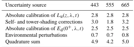
An analysis of uncertainties of WiSPERRrs(λ)from ARC measurements, performed assuming each contribution inde-pendent from the others, indicates values in the range of ap-proximately 4–5 % in the selected spectral region (see Ta-ble 3). The uncertainty sources considered here are (i) un-certainty of the absolute radiance calibration (Hooker et al., 2002b) and immersion factor (Zibordi, 2006) for theLu sen-sor (i.e. 2.7 % and 0.5 %, respectively, composed statisti-cally); (ii) uncertainty of the correction factors applied for removing self-shading and tower-shading perturbations com-puted as 25 % of the applied corrections; (iii) uncertainty of the absolute irradiance calibration of the above-waterEd sen-sor (Hooker et al., 2002b) and uncertainties of the correction applied for the non-cosine response of the related irradiance collectors (Zibordi and Bulgarelli, 2007) (i.e. 2.3 % and 1 %, respectively, composed statistically); (iv) uncertainty in the extrapolation of sub-surface values due to wave perturbations and changes in illumination and seawater optical properties during profiling cumulatively quantified as the average of the variation coefficient ofRrs(λ)from replicate measurements.
It is noted that the proposed uncertainty analysis accounts for fully independent calibrations ofEdandLusensors (i.e.
Table 3. Uncertainty budget (in percent) forRrsdetermined from
WiSPER data.
Uncertainty source 443 555 665
Absolute calibration ofLu(z, λ, t) 2.8 2.8 2.8
Self- and tower-shading corrections 3.0 1.8 3.2 Absolute calibration ofEd(0+, λ, t) 2.5 2.5 2.5
Environmental perturbations 0.7 0.7 0.8
Quadrature sum 4.9 4.2 5.0
as obtained with different lamps and laboratory set-ups). The use of the same calibration lamp and set-up leads to a reduc-tion of approximately 1 % of the quadrature sum of spectral uncertainties for WiSPERRrs(λ).
indicates maximum values smaller than 0.5 % forRrs at the 555 nm center-wavelength.
The quality of WiSPER radiometric products is traced through quality-indices determined during data processing. These include (i) temporal changes in illumination condi-tions as caused by cloudiness and quantified through the standard deviation of Ed(0+, λ, t ) at each λ; (ii) poten-tial difficulties in the determination of subsurface extrap-olated quantities flagged by a relatively small number of measurements per unit depth, significant differences between
Eu(z, λ, t0)/Lu(z, λ, t0)at different depths in the extrapola-tion interval, and large differences betweenEd(0−, λ, t0)and Ed(0+, λ, t0); and (iii) poor illumination conditions, result-ing from high sun zenith angles or cloudiness, both quanti-fied through values of the diffuse to direct irradiance ratio
r(λ)exceeding a threshold. These quality-indices, recorded as an integral part of the radiometric data set, are used to comprehensively qualify data products. The low deployment speed of WiSPER and the almost ideal sky and sea state con-ditions characterizing the ARC measurements made all the collected data applicable for the inter-comparison.
3.3.2 TACCS
The Tethered Attenuation Chain Colour Sensors (TACCS) manufactured by Satlantic Inc. consist of an above-waterEd sensor mounted on a buoy, anLuupwelling radiance sensor at depthz0=0.5 m, and a chain of four in-waterEdsensors at increasing depthszi. A weight suspended at the bottom of the chain stabilises the system against wave action. TACCS offers the advantage of easy deployment from small boats and the possibility of being operated at distances minimizing ship perturbations. Additionally,Lu(z0, λ, t) data taken rela-tively close to the surface can be averaged over time to mini-mize the effects of wave focussing and defocusing. The main disadvantage is the reduced depth resolution with respect to profilers, requiring a careful quality check of data to exclude cases affected by near-surface vertical non-homogeneities.
Individual measurement sequences comprise collection of
Lu(z0, λ, t),Ed(zi, λ, t )andEd(0+, λ, t )during intervals of three minutes. Measurement sequences are retained and cor-rected using Eq. (1) for the effects of illumination change during data collection when the variability ofEd(0+, λ, t )is no greater than 2.5 % with sea state 0–1, 3.0 % with sea state 1–2, or 4 % with sea state 4 (essentially, the variability should be consistent with wave action rather than with changes in illumination which have a higher frequency). Derived
Lu(z0, λ, t0)andEd(zi, λ, t0)are then averaged over the three minute interval to determine time-averagedL¯u(z0, λ, t0)and
¯
Ed(zi, λ, t0), respectively.
Log transformedE¯d(zi, λ, t0)are then applied to compute Kd(λ) through least-squares linear regressions. Because of the similarity of Kl(λ) and Kd(λ) values (Mobley, 1994),
subsurfaceLu(0−,λ)is then obtained from: Lu(0−, λ)=
¯
Lu(z0, λ, t0)
e−z0Kd(λ) . (6)
Quality checks for Lu(0−, λ) include the evaluation of R2 determined from the regression ofE¯d(zi, λ, t0)at depthszi and the visual inspection ofE¯d(zi,490, t0)profile data. IfR2 and the vertical profile of log-transformedE¯
d(zi,490, t0) in-dicate non-homogeneity of the optical properties in the water column, then the lowest depth(s) are removed from the pro-cessing. These steps aim to ensure the validity of the hypoth-esis of homogeneous seawater optical properties between the surface and at least the second measurement depth.
Self-shading corrections ofLu(0−, λ)data are performed following the methodology detailed by Mueller et al. (2002). Input quantities are (i) the total seawater absorption coeffi-cienta(λ), on a first approximation assumed equal toKd(λ) (Mobley, 1994) directly determined from Ed(zi, λ, t ) val-ues; (ii) the diameter of the Lu sensor (by neglecting the marginal effects of the surface float (Moore et al., 2010)); and (iii) the diffuse to direct irradiance ratior(λ)calculated from simulated data using the model of Bird and Riordan (1986) with extra-atmospheric sun irradiance from Thuillier et al. (2003) and aerosol optical thickness τa(λ) from col-located sun-photometric measurements. Comparison of self-shading corrections determined for ARC measurement con-ditions with the former 2-D scheme (where the system is assumed a disk with diameter equal to the case of the Lu sensor) and corrections from a 3-D scheme developed by Leathers et al. (2001) for an equivalent buoy system indi-cates differences well within the 35 % uncertainty declared for the 2-D based scheme (see the following subsections).
Two TACCS systems were deployed during the ARC inter-comparison: one owned and managed by Stockholm Univer-sity in collaboration with Bio-Optika (identified as TACCS-S), and the second by Sagremarisco Lda also in collaboration with Bio-Optika (identified as TACCS-P). Although the two TACCS systems have different radiometric configurations, the mechanical design is almost identical.
During the ARC activities both TACCS were operated at a few meters from each other at approximately 30 m from the AAOT.
TACCS-S
TACCS-S measures Ed(0+, λ, t) at 443, 490 and 670 nm, andEd(zi, λ, t) at 490 nm at the nominal depths of 2, 4, 6 and 8 m. Measurements ofLu(z0, λ, t) are performed at 412, 443, 490, 510, 560, 620 and 670 nm at the nominal depth
z0=0.5 m with an in water FAFOV of approximately 20◦. All sensors have a 10 nm bandwidth. The acquisition rate is approximately 1 Hz.
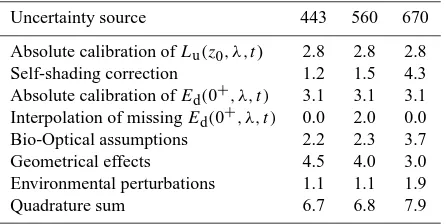
Table 4. Uncertainty budget (in percent) forRrs determined from
TACCS-S data.
Uncertainty source 443 560 670
Absolute calibration ofLu(z0, λ, t) 2.8 2.8 2.8
Self-shading correction 1.2 1.5 4.3
Absolute calibration ofEd(0+, λ, t ) 3.1 3.1 3.1
Interpolation of missingEd(0+, λ, t ) 0.0 2.0 0.0
Bio-Optical assumptions 2.2 2.3 3.7
Geometrical effects 4.5 4.0 3.0
Environmental perturbations 1.1 1.1 1.9
Quadrature sum 6.7 6.8 7.9
Since Ed(0+, λ, t ) is only measured at 443, 490 and 670 nm, simulated irradiances (computed using the same model utilized for the determination ofr)are normalized to the actualEd(0+, λ, t )to determine values at 412, 510, 560 and 620 nm.
Similarly, sinceKd(λ)is only measured at 490 nm, spec-tral values ofKd(λ)at the relevant center-wavelengths are determined from measurements ofa(λ) andc(λ) performed with an AC-9 (WET Labs, Philomath, USA) following Kirk (1994) with:
Kd(λ)=µ−01[a(λ) 2+(g
1µ0−g2)a(λ)b(λ)]0.5, (7) whereb(λ)=c(λ)−a(λ),µ0is the mean cosine of the re-fracted solar beam just below the sea surface, andg1 and g2constants depend on the scattering phase function. For the processing of ARC data, constant values areµ0=0.86,g1= 0.425, and g2=0.19 corresponding to the Petzold (1972) phase function. It is assumed that these parameters provide the correct spectral shape of Kd(λ), although its absolute value may be biased due to dependence ofµ0onθ0.
The analysis of uncertainties for TACCS-SRrs(λ) from ARC measurements indicates values in the range of approx-imately 7–8 % (see Table 4). Considered uncertainty sources are (i) uncertainty of the absolute radiance calibration and immersion factor, computed as for WiSPER; (ii) uncertainty of the correction factors applied for removing self-shading perturbations in Lu(0−, λ) computed as 35 % of the ap-plied corrections (the higher expected values with respect to WiSPER are explained by the assumption ofa(λ)=Kd(λ)); (iii) uncertainty of the absolute irradiance calibration of the above-waterEdsensor (Hooker et al., 2002b) and non-cosine response of the related irradiance collectors (Zibordi and Bulgarelli, 2007) (i.e. 2.3 % and 2 %, respectively, com-posed statistically); (iv) uncertainty in the determination of
Ed(0+, λ, t) at missing center-wavelengths estimated by cal-culatingEd(0+, λ, t) using the model of Bird and Riordan (1986) withτa(500)=0.45 (average for measurements per-formed during the field activities) and by bracketing the
˚
Angstr¨om exponent at 0.0 and 2.0; (v) uncertainties due to the assumption ofKl(λ)=Kd(λ)resulting from the quadra-ture sum of 1.7 %, average difference between Kd(λ) and
Kl(λ)determined through Hydrolight (Mobley, 1998) sim-ulations using the specific TACCSEdsensor depths, and of approximately 1.7 % per 100 nm due to spectral extrapola-tion as estimated from actual measurements; (vi) uncertain-ties due to geometrical effects estimated from simulations, assuming tilt of 5◦ for the above-waterEd sensor, relative sun-sensor azimuth of 180◦,θ0=45◦,r(λ) computed with τa(500)=0.45 and ˚Angstr¨om exponent equal to 1.39 as re-sulting from measurements performed during field activities; and (vii) uncertainty in the extrapolation of sub-surface val-ues, computed as for WiSPER.
Uncertainties do not take into account potential shading of the in-water Ed sensors by the cable. This is supported by the assumption that this perturbation similarly affects mea-surements at all depths and thus does not significantly influ-ence the determination ofKd(λ). No uncertainty has been as-signed to the nominal depths of in-waterEdsensors assumed to be within±2 cm under calm sea.
Finally, in view of the inter-comparison analysis, it is anticipated that differences between TACCS-S center-wavelengths at 560 and 670 nm with respect to the reference ones at 555 and 665 nm are neglected.
TACCS-P
TACCS-P has hyperspectral sensors for Ed(0+, λ, t) and Lu(z0, λ, t) measurements with spectral range of 350– 800 nm and resolution of 11 nm. TheLusensor has in-water FAFOV of approximately 18◦. Ed(zi, λ, t ) is measured at 412, 490, 560 and 665 nm with a bandwidth of 10 nm at nominal depths of 2, 4, 8 and 16 m. Sampling rate is typi-cally 2 Hz, although it may vary depending on illumination conditions. Tilt and compass sensors provide information on the levelling and orientation of the radiometer utilized for
Ed(0+, λ, t) measurements.
Since Kd(λ) is only determined at 412, 490, 560 and 665 nm, at the other relevant center-wavelengths it is deter-mined with the following scheme. The value of Chlais esti-mated fromKd(490) by inverting Eq. (9) from Morel and An-toine (1994), duly taking into account the diffuse attenuation coefficient of pure seawater. Then the same equation with the estimated Chlais applied to determine the diffuse atten-uation coefficient of seawater (pure seawater excluded). The derivedKd(λ) spectrum is subsequently normalised to the ex-perimental values determined at 412, 490, 560 and 665 nm.
Ed(0+,λ, t )is calculated by two methods depending on tilt values during the sampling period. The value ofEd(0+,λ, t ) is kept unchanged if the combined x-y tilt value is less than 2◦. Otherwise a correction is applied by assuming that the diffuse irradiance is unaffected by tilt (i.e. by ignoring the sky radiance distribution) according to:
Ed(0−, λ, t )=
Ed(0−, λ, t, θs) 1+f (θ0,θs)−1
1+r(λ)
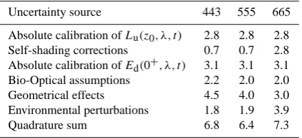
Table 5. Uncertainty budget (in percent) forRrsdetermined from
TACCS-P data.
Uncertainty source 443 555 665
Absolute calibration ofLu(z0, λ, t) 2.8 2.8 2.8
Self-shading corrections 0.7 0.7 2.8
Absolute calibration ofEd(0+, λ, t ) 3.1 3.1 3.1
Bio-Optical assumptions 2.2 2.0 2.0
Geometrical effects 4.5 4.0 3.0
Environmental perturbations 1.8 1.9 3.9
Quadrature sum 6.8 6.4 7.3
whereEd(0−, λ, t, θs)indicates data uncorrected for tilt and f (θ0, θs)is given by:
f (θ0, θs)= cos(θs) cos(θ0)
, (9)
withθsthe apparent angle of the sun to the collector plane of the irradiance sensor.
This correction, however, only applies to tilts less than 8◦ (chosen on the basis of trials performed under stable illumi-nation conditions). In fact, when the tilt becomes high the radiance from the sea surface may add large perturbations, especially in the anti-solar direction.
The analysis of uncertainties for TACCS-PRrs(λ) from ARC measurements indicates values in the range of approx-imately 6–7 % (see Table 5). Considered uncertainty sources are (i) uncertainty of the absolute radiance calibration and immersion factor of the Lu sensor, computed as for WiS-PER; (ii) uncertainty in the correction factors applied for re-moving self-shading perturbations inLu(z0, λ, t), computed as for TACCS-S; (iii) uncertainty of the absolute irradiance calibration of the above-waterEdsensor and the non-cosine response of the related irradiance collectors, computed as for TACCS-S; (iv) uncertainties due to the assumption of
Kl(λ)=Kd(λ), computed as for TACCS-S; (v) uncertainties due to geometrical effects computed as for TACCS-S; and (vi) uncertainty due to the extrapolation of sub-surface val-ues, computed as for WiSPER.
3.3.3 SeaPRISM
The SeaWiFS Photometer Revision for Incident Sur-face Measurements (SeaPRISM) is a modified CE-318 sun-photometer (CIMEL, Paris) that has the capabil-ity of performing autonomous above-water measurements. SeaPRISM is regularly operated at the AAOT from a de-ployment platform located in the western corner of the su-perstructure at approximately 15 m above the sea level (Zi-bordi et al., 2009c). Measurements performed with a FAFOV of 1.2◦ every 30 min for the determination of Lw(λ) at a number of center-wavelengths including 412, 443, 488, 531, 551, 670 nm (Zibordi et al., 2009c) are (i) the direct sun irra-dianceEs(θ0, φ0, λ) acquired to determine the atmospheric
optical thickness τa(λ) used for the theoretical computa-tion of Ed(0+, λ), and (ii) a sequence of 11 sea-radiance measurements for determiningLT(θ, 1φ, λ) and of 3 sky-radiance measurements for determiningLi(θ0, 1φ, λ). These sequences are serially repeated for eachλ with1φ=90◦,
θ=40◦ andθ0=140◦. The larger number of sea measure-ments, when compared to sky measuremeasure-ments, is required be-cause of the higher environmental noise (mostly produced by wave perturbations) affecting the former measurements dur-ing clear sky.
Values of Rrs(λ) are determined from SeaPRISM mea-surements in agreement with basic principles provided in Sect. 3.2. An additional element is the need to minimize the effects of glint perturbations in LT(θ, 1φ, λ) and possibly the effects of cloud perturbations in Li(θ0, 1φ, λ). This is achieved by deriving these values from the average of inde-pendent measurements satisfying strict filtering criteria (Zi-bordi et al., 2009c; Zi(Zi-bordi, 2012).
Finally, as already anticipated, the value ofEd(0+,λ)is quantified theoretically under the assumption of clear sky. Specifically,
Ed(0+, λ)=E0(λ)D2td(λ)cosθ0 , (10) whereD2accounts for the variations in the Sun–Earth dis-tance as a function of the day of the year (Iqbal, 1983),td(λ) is the atmospheric diffuse transmittance computed from mea-sured values ofτa(λ) (Gordon and Clark, 1981), andE0(λ) is the average extra-atmospheric sun irradiance (Thuillier et al., 2003).
Quality flags are applied at the different processing lev-els to remove poor determinations of Rrs(λ). Quality flags include checking for (see Zibordi et al., 2009c) cloud con-tamination, high variance of multiple sea- and sky-radiance measurements, elevated differences between pre- and post-deployment calibrations of the SeaPRISM system, and spec-tral inconsistency of the normalized water-leaving radiance
Lwn(λ)given by:
Lwn(λ)=Rrs(λ)E0(λ). (11)
It is recalled that SeaPRISM data, handled through the Ocean Color component of the Aerosol Robotic Network (AERONET-OC, Zibordi et al., 2009c), are mostly intended to support satellite ocean color validation activities. Because of this, to minimize the effects of differences in center-wavelengths between the satellite and SeaPRISM data prod-ucts a band-shift correction scheme has been developed for the latter. These corrections are performed relying on a bio-optical model requiring Chl a and IOP values estimated through regional empirical algorithms applied to spectral ra-tios ofLwn(λ) (Zibordi et al., 2009b). Band-shift corrections have then been applied to SeaPRISM data products con-tributing to the ARC inter-comparison to match the reference center-wavelengths.
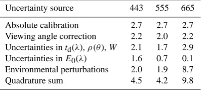
Table 6. Uncertainty budget (in percent) forRrsdetermined from
SeaPRISM data.
Uncertainty source 443 555 665
Absolute calibration 2.7 2.7 2.7
Viewing angle correction 2.2 2.0 2.2
Uncertainties intd(λ),ρ(θ),W 2.1 1.7 2.9
Uncertainties inE0(λ) 1.6 0.7 0.1
Environmental perturbations 2.0 1.9 8.7
Quadrature sum 4.5 4.2 9.8
is justified by its continuous operation for periods of 6–12 months at the AAOT. However, pre- and post-deployment calibrations performed at the JRC with the same standards and methods applied during ARC indicated differences typi-cally within 0.6 % during a 9 month period.
Estimated uncertainties of SeaPRISMRrs(λ) data for the ARC experiment are approximately 4–5 % in the blue-green spectral regions and 10 % in the red (see Table 6). These have been determined accounting for contributions from (i) uncertainty of the absolute radiance calibration (Hooker et al., 2002b) for LT andLi sensors, but neglecting sensi-tivity changes during deployment which should contribute less than 0.2 % when assuming a linear change with time between pre- and post-deployment calibrations; (ii) uncer-tainty of corrections for the off-nadir viewing geometry com-puted as 25 % of the applied correction factors (these rela-tively large percent values are expected to account for un-certainties due to the intrinsic assumption of Case 1 wa-ter at the AAOT); (iii) variability in specific paramewa-ters re-quired for the determination ofRrs(λ) (taken from Zibordi et al., 2009c, and estimated from multi-annual measuments accounting for changes in wind speed, sea surface re-flectance, and atmospheric diffuse transmittance); (iv) uncer-tainty inE0(λ) estimated by assuming±1 nm uncertainty in center-wavelengths; and finally, (v) environmental perturba-tions (e.g. wave effects, changes in illumination and seawater optical properties during measurements) quantified as the av-erage of the variation coefficient obtained fromRrs(λ) values from replicate measurements.
The uncertainty related to band-shift corrections has not been accounted for in the overall budget. However, an eval-uation of band-shift corrections applied to SeaPRISM data to match center-wavelengths of various satellite sensors indi-cated average values of a few percent (Zibordi et al., 2006). Thus, the uncertainty affecting these values is expected to be a small fraction of the applied corrections and consequently to not significantly impact the uncertainty budget proposed for SeaPRISMRrs(λ).
3.3.4 TRIOS
Above-water TriOS (Rastede, Germany) Optical Sys-tems (TRIOS) are composed of two RAMSES
ARC-VIS hyperspectral radiometers measuringLT(θ, 1φ, λ) and Li(θ0, 1φ, λ), and one RAMSES ACC-VIS forEd(0+,λ). Measurements are performed in the 400–900 nm spectral range with resolution of about 10 nm for the output data. The nominal FAFOV of radiance sensors is 7◦.
The basic measurement method applied during ARC is that developed by Ruddick et al. (2006, see the main pa-per and web appendices) based on the generic Method 1 de-scribed in the Ocean Optics Protocols (Mueller et al., 2002).
LT and Li sensors are simultaneously operated on the same frame with identical azimuth plane, and θ=40◦ and
θ0=140◦, respectively. Measurement sequences are per-formed with user-definable intervals and frequencies, and in-tegration time varying automatically between 8 ms and 4 s depending on the brightness of the target. During ARC, the deployment frame was adjusted for each measurement se-quence to satisfy the requirement of 1φ=135◦ (or occa-sionally of1φ=90◦, chosen to avoid superstructure pertur-bations).
Details on data processing, including measurement selec-tion, averaging and quality checks, are described in Ruddick et al. (2006) (web appendix 1: http://aslo.org/lo/toc/vol 51/ issue 2/1167a1.pdf). A few elements on data processing are however provided here for completeness.
Following Ruddick et al. (2006) and in agreement with Sects. 3.2 and 3.1, the remote sensing reflectance
Rrs0(θ, 1φ, λ)for individualLT(θ, 1φ, λ) andLi(θ0, 1φ, λ) measurements is computed as:
Rrs0(θ, 1φ, λ)=LT(θ, 1φ, λ)−ρ 0(W ) L
i(θ0, 1φ, λ) Ed(0+, λ)
, (12) where ρ0(W ) indicates the sea surface reflectance during clear sky conditions, solely expressed as a function ofW (in units of m s−1),
ρ0(W )=0.0256+0.00039W+0.000034W2. (13) Minimization of perturbations due to wave effects is then achieved through the so-called turbid water near-infrared (NIR) similarity correction (Ruddick et al., 2005) by deter-mining the departure from the NIR similarity spectrum with:
ε=α·R 0
rs(θ, 1φ, λ2)−R0rs(θ, 1φ, λ1)
α−1 , (14)
where wavelengthsλ1andλ2are chosen in the near infrared and the constantαis set accordingly from Table 2 of Rud-dick et al. (2006). It is noted that this scheme is similar to that proposed by Gould et al. (2001), although relying on different wavelengths and values ofαand of the sea surface reflectance.
The NIR similarity corrected remote sensing reflectance
Rrs(θ, 1φ, λ)is then calculated from:
Table 7. Uncertainty budget (in percent) forRrsdetermined from
TRIOS-B data.
Uncertainty source 443 555 665
System calibration 2.0 2.0 2.0
Straylight effects 5.0 0.5 1.0
Polarization effects 1.0 1.0 1.0
Non-cosine response ofEd 2.0 2.0 2.0
Sky-light correction 2.0 1.0 2.9
Viewing angle correction 1.5 1.5 1.5
Quadrature sum 6.3 3.5 4.5
where the correction is assumed spectrally invariant. The cor-responding NIR similarity corrected water-leaving radiance is calculated as:
Lw(θ, 1φ, λ)=Ed(0+, λ)Rrs(θ, 1φ, λ). (16) A number of data products (i.e. 5) are then averaged to obtain the NIR similarity correctedL¯w(θ, 1φ, λ).
For ARC measurements a viewing angle correction is also applied toL¯w(θ, 1φ, λ)in agreement with Eq. (5) to deter-mineLw(λ). The values of Chla required for such a cor-rection were estimated using a regional band-ratio algorithm (Berthon and Zibordi, 2004).
Two TRIOS systems were deployed at the AAOT adjacent to the SeaPRISM during the ARC experiment: one owned and handled by the Management Unit of the North Sea Math-ematical Models (identified as TRIOS-B) and the other by Tartu Observatory (identified as TRIOS-E). The two sys-tems are equivalent, but measurements have been performed independently and reduced by applying slightly different schemes, corresponding to the standard practices of the two institutions and with some differences in the approach for un-certainty estimate. These elements are separately presented in the following subsections.
Data for inter-comparisons have been constructed by lin-early interpolating quality checked products at the reference center-wavelengths.
TRIOS-B
Ed(0+, λ), LT(θ, 1φ, λ) and Li(θ0, 1φ, λ) are simultane-ously acquired for 10 min taking measurements every 10 s. Calibrated data are quality checked for incomplete and for in-dividual measurements differing by more than 25 % from the neighbouring ones. In the case of ARC data, quality check-ing led to the rejection of 1 % of measurements. The NIR similarity correction is then performed using λ1=780 nm, λ2=870 nm, andα=1.91 (Ruddick et al., 2006).
Estimated uncertainties ofRrs(λ) for TRIOS-B approxi-mately vary between 4 and 6 % in the spectral range of in-terest (see Table 7). The considered uncertainty sources are (i) uncertainty of system calibration determined assuming the same irradiance standard is utilized for the absolute
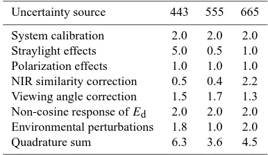
cal-Table 8. Uncertainty budget (in percent) forRrs determined from
TRIOS-E data.
Uncertainty source 443 555 665
System calibration 2.0 2.0 2.0
Straylight effects 5.0 0.5 1.0
Polarization effects 1.0 1.0 1.0
NIR similarity correction 0.5 0.4 2.2 Viewing angle correction 1.5 1.7 1.3 Non-cosine response ofEd 2.0 2.0 2.0
Environmental perturbations 1.8 1.0 2.0
Quadrature sum 6.3 3.6 4.5
ibration of the Ed, LT, and Li sensors, and thus only ac-counting for effects of mechanical setup, inadequate baf-fling and reference plaque uncertainties (see Hooker et al., 2002b); (ii) uncertainty due to straylight effects quantified through the application of laboratory characterizations per-formed for RAMSES Ed, LT andLi sensors (Ansko, un-published); (iii) polarization effects quantified as the max-imum sensitivity to polarization determined through labo-ratory characterizations for RAMSES LT and Li sensors (Ruddick, unpublished); (iv) effects of non-cosine response of the above-water Ed collector determined from labora-tory measurements (Ruddick, unpublished); (v) uncertainty in sky-light correction quantified in agreement with Ruddick et al. (2006) as a function of the uncertainty inρ0(W ); and (vi) uncertainty in the correction for off-nadir viewing angle quantified as 25 % of the applied corrections, and exhibit-ing different values than those proposed for SeaPRISM be-cause of the diverse viewing geometry generally relying on
1φ=135◦instead of1φ=90◦.
It is noted that the uncertainty for the sky glint correction is highly dependent on sea state, and the relative percent value of this uncertainty is inversely proportional toRrs(θ, 1φ, λ) (see web appendix 2 of Ruddick et al., 2006). The values given here have, therefore, been calculated very specifically accounting for the sea state recorded during the ARC activ-ities and the observed water-leaving radiances (see Sect. 4). Measurements performed in different waters or sea state con-ditions may lead to different uncertainties.
TRIOS-E
0.00 0.25 0.50 0.75 1.00
400 500 600 700 Lw
[mW cm
-2
PP
m
-1 sr -1]
Wavelength [nm]
Fig. 1.Lw(λ)spectra from WiSPER produced during the ARC
ex-periment at the AAOT.
Quality checks rely on the mode ofRrs(555) for each mea-surement sequence. Data deviating by more than 10 % from the mode value are rejected; actually none of the clear sky data included in the ARC inter-comparison was discarded.
Estimated uncertainties ofRrs(λ)from TRIOS-E vary ap-proximately within 4–6 % (see Table 8). The considered un-certainty sources are (i) unun-certainty of system calibration, computed as for TRIOS-B; (ii) uncertainty due to straylight effects, computed as for TRIOS-B; (iii) polarization effects, computed as for TRIOS-B; (iv) uncertainty in the turbid wa-ter NIR similarity correction quantified accounting for 25 % of the applied corrections; (v) uncertainty in the correction for off-nadir viewing angle (also estimated as 25 % of the applied corrections); (vi) effects of non-cosine response of theEd collector guessed from published data (Zibordi and Bulgarelli, 2007); and (vii) environmental perturbations esti-mated from the variation coefficient ofRrs(λ)from the same measurement sequence.
4 Data analysis and results
The inter-comparison analysis has been performed using matchups (i.e. pairs of data products from different sys-tems) constructed by setting±15 min maximum difference between measurements from the two systems/methods to be compared. Matchup analysis has been performed through the average of relative and of absolute values of percent differ-ences. Specifically, the average of relative percent differences (RD) is computed as:
RD=1001
N
N
X
n=1
<C(n)− <R(n)
<R(n) , (17)
while the average of absolute values of percent differences (AD) is given by:
AD=1001
N
N
X
n=1
<C(n)− <R(n)
<R(n) , (18)
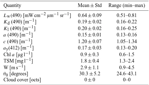
Table 9. Values of major quantities characterizing the measurement conditions during ARC activities at the AAOT.
Quantity Mean±Std Range (min–max)
Lw(490)[mW cm−2µm−1sr−1] 0.64±0.09 0.51–0.81
Kd(490) [m−1] 0.19±0.02 0.16–0.22
Kl(490) [m−1] 0.20±0.02 0.16–0.25
a(490) [m−1] 0.15±0.01 0.13–0.16
c(490) [m−1] 1.20±0.07 1.05–1.34
ay(412) [m−1] 0.17±0.03 0.13–0.20
Chla[µg l−1] 0.9±0.3 0.6–1.5
TSM [mg l−1] 1.8±0.4 1.3–2.4
W [m s−1] 2.9±1.1 0.9–4.5
θ0[degrees] 30.3±5.2 24.6–43.1
Cloud cover [octs] 0±0 0–0
whereNis the number of matchups,nis the matchup index, superscriptC indicates the quantity to be compared, and su-perscriptRindicates the reference. While RD is applied as an index to measure biases, AD is applied to quantify scattering between compared values.
The root mean square of differences (RMS),
RMS= v u u t
1
N
N
X
n=1
(<C(n)− <R(n))2, (19)
is also included in the analysis as a statistical index to quan-tify differences in absolute units.
Data products from WiSPER are applied as the refer-ence. This choice is only supported by the confidence ac-quired with the system and the related measurement method. WiSPER data for ARC inter-comparisons comprise measure-ments from 36 independent casts performed under clear sky conditions from 21 to 24 July 2010. DerivedLw(λ) spec-tra are given in Fig. 1. The shape of specspec-tra suggests a wa-ter type characwa-terized by moderate concentrations of phyto-plankton and colored dissolved organic matter, as shown by the decrease of spectra from 555 nm toward 412 nm, and ad-ditionally, moderate concentration of total suspended mat-ter, as shown by non-negligible values at 665 nm. An evalu-ation of the water type made in agreement with Loisel and Morel (1998) indicates the presence of Case 2 water dur-ing the whole field experiment. Values for relevant quanti-ties describing measurement conditions are reported in Ta-ble 9. Specifically, measurements performed on water sam-ples collected during ARC activities at the AAOT indicate average Chla values of 0.9±0.3 µg l−1, concentrations of total suspended matter (TSM) of 1.8±0.4 g l−1, and absorp-tion coefficient by colored dissolved organic matter ay at 412 nm of 0.17±0.03 m−1. However, despite the relative constancy of near surface quantities, the analysis ofa(λ)and
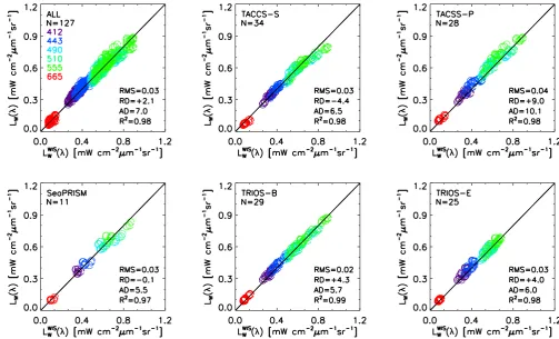
Fig. 2. Scatter plots ofLw(λ)from the various systems/methods versusLw(λ)from WiSPER (ALL indicates merged data from all individual
inter-comparisons). RMS indicates the spectrally averaged root mean square of relative differences, while RD and AD in % indicate spectrally averaged values of relative differences and of absolute values of relative differences, respectively.Nis the number of matchups, all obtained assuming a±15 min maximum difference between measurements. Diverse colors indicate data at different center-wavelengths.
exclusion from data processing of the measurements related to these depths has minimized potential inconsistencies in the inter-comparison of products likely affected by the non-linear decay with depth of log-transformedLu(z, λ, t0)and Ed(z, λ, t0)data.
By recalling that the objective of the inter-comparison is the evaluation of the overall performance of different sys-tems/methods regularly applied for satellite ocean color vali-dation activities, and not a detailed investigation of any indi-vidual method, a summary of inter-comparison results is pre-sented through scatter plots in Figs. 2–4 forLw(λ),Ed(0+, λ) andRrs(λ), respectively. The different number of matchups included in the analysis for the various systems/methods is explained by practical deployment issues for various systems on some days, such as the application of the±15 min thresh-old not always being reached because of inadequate synchro-nization of the start of measurement sequences, or like in the case of SeaPRISM data, justified by the automatic and fully asynchronous (when compared to ARC activities) ex-ecution of measurements. It is however reported that most of the TRIOS-B and TRIOS-E measurements used to con-struct matchups are within±1 min from WiSPER
measure-ments, while most of TACCS-S and TACCS-P measurements are within±3 min.
Inter-comparisons ofLw(λ)displayed in Fig. 2 exhibit val-ues of RMS in the range of 0.02–0.03 mW cm−2µm−1sr−1, except TACCS-P reaching 0.04 mW cm−2µm−1sr−1. Spec-trally averaged values of RD and AD are generally within ±4 % and 5–7 %, respectively. Higher values (i.e. +9 and 10 %) are observed for TACCS-P. Determination coefficients,
R2, exhibit values higher than 0.98, except for the SeaPRISM data whereR2=0.97.
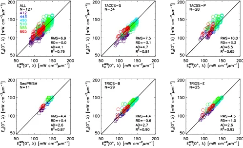
Fig. 3. As in Fig. 2 but forEd(0+,λ).
when considering that SeaPRISMEd(0+,λ)data are deter-mined theoretically from experimental values ofτa(λ), a very different approach from actual measurements applied for all other systems/methods. Values of RD forEd(0+,λ)are ap-proximately within ±3 % while values of AD are close to 3 % for the above-water systems (e.g. SeaPRISM, TRIOS-B and TRIOS-E), but reach 5–7 % for the buoy-based sys-tems/methods (i.e. TACCS-S and TACCS-P). Similarly,R2
vary between 0.87 and 0.92 for the above-water systems, and exhibit much lower values for TACCS-S and TACCS-P (i.e.
R2equal to 0.81 and 0.65, respectively).
The inter-comparison shown in Fig. 4 for Rrs(λ) data exhibits results obviously depending on those obtained for
Lw(λ) andEd(0+, λ)data. Specifically, lower RMS values (i.e. 0.0002 sr−1)are shown for TRIOS-B and TRIOS-E, and the highest (i.e. 0.0004 sr−1)for TACCS-P. RD values vary from−1 to+6 %, while AD values are approximately 6 % for the above-water systems and reach 9 % for the buoy-based systems. AllR2vary between 0.95 and 0.99 with the lowest values again displayed by the S and TACCS-PRrs(λ)as a result of the lowerR2shown byEd(0+, λ).
The former analysis efficiently summarizes the general performances of the various systems/methods, but limits the possibility of evaluating the spectral performances at the se-lected center-wavelengths. The inter-comparison analysis is then completed with the presentation of spectral statistical
indices for each system/method in Tables 10–12 forLw(λ), Ed(0+,λ)andRrs(λ), respectively. These data show various peculiarities. For instance,R2determined from spectral val-ues of Lw(λ) andRrs(λ) are much lower than those com-puted with spectrally combined data (e.g. note the striking values for SeaPRISM Lw at 443 nm). This is undoubtedly explained by the small range characterizing the spectral val-ues ofLw(λ)due to the low variability of the seawater bio-optical properties (see Table 9). When looking at Table 10, also relevant are the biases affecting TACCS-S and TACCS-P (i.e.−20 % and+21 %, respectively) and also TRIOS-B and TRIOS-E (i.e.+12 % and+10 %, respectively) at 665 nm. These are likely explained by the difficulty in determining near surfaceKd(665) for TACCS and by imperfect sky-glint removal for TRIOS.
Fig. 4. As in Fig. 2 but forRrs(λ).
4.1 Discussion
Results for the ARC inter-comparison illustrate the best that can be achieved with the considered systems/methods under almost ideal measurement circumstances driven by favourable deployment capabilities as offered by the stability of the AAOT platform (i.e. makingEd(0+,λ)measurements unaffected by tilt, when performed from the main superstruc-ture), almost ideal environmental conditions characterized by relatively low sun zenith angles, clear sky and moder-ately low sea state, and finally inter-calibration of measure-ment systems. By solely considering this latter elemeasure-ment, it is recalled that the inter-calibration removes potential biases in derived radiometric products generated by out-of-date or inaccurate calibrations. The comparison of absolute coeffi-cients obtained at the JRC during the inter-calibration with those previously applied for the various systems included in ARC has shown minimum differences of 1–2 % but also values exceeding 4 % for individual radiometers. These sec-ond relatively high differences, if not removed, would signifi-cantly degrade the inter-comparison for one of the considered systems/methods.
Processing of data from in-water systems/methods re-quires values of a(λ) and c(λ). Differently, processing of data from above-water systems/methods requires valuesW
and Chla. The impact of uncertainties of these input
quanti-ties is accounted for in theRrs(λ)uncertainty budget for each system/method. It is however of interest to evaluate the im-pact of important quantities such as Chlautilized to correct for the off-nadir viewing geometry ofLw(θ, 1φ, λ). In the present exercise Chlawas determined for all systems using a regional algorithm (see Berthon and Zibordi, 2004) applied toRrs(λ) ratios. The average and the standard deviation of values computed for ARC measurements are 1.9±0.2 µg l−1. The corresponding values for actual concentrations deter-mined from water samples through High Performance Liquid Chromatography (HPLC) are 0.9±0.3 µg l−1. The analysis of TRIOS-B data indicates that the different Chlaestimates give viewing angle corrections differing by less than 1 % for
1φ=135◦ and varying between 1 and 4 % for 1φ=90◦. However, the overall effect on Rrs(λ) inter-comparisons is well within the assumed uncertainties. In fact, when using measured Chl a instead of the computed values, TRIOS-E, TRIOS-B and SeaPRISM results indicate an increase of 0.5 %, 0.9 % and 1.2 %, respectively, for the spectrally av-eraged RD, and no significant change for the other statistical quantities. Differences among spectrally averaged RD for the various systems/methods are explained by the different mea-surement sequences included in the inter-comparison com-prising diverse viewing geometries.
Table 10. Spectral values of the statistical indices (i.e. RMS, RD, AD andR2) quantifying the inter-comparison results forLw(λ)at the 443,
555 and 665 nm center-wavelengths for the various systems/methods with respect to WiSPER.
443 555 665
N RMS RD AD R2 RMS RD AD R2 RMS RD AD R2
TACCS-S 34 0.02 0.2 3.1 0.87 0.04 −2.9 4.5 0.90 0.02 −20.0 20.0 0.85
TACCS-P 28 0.04 8.8 9.7 0.67 0.06 7.9 8.2 0.91 0.02 21.3 21.5 0.81
SeaPRISM 11 0.03 1.5 5.1 0.07 0.04 1.1 4.1 0.88 0.01 −3.6 7.1 0.56
TRIOS-B 29 0.03 5.7 5.9 0.92 0.02 1.6 2.5 0.98 0.01 12.3 12.3 0.96
TRIOS-E 25 0.03 5.4 6.1 0.61 0.02 1.8 2.8 0.82 0.01 10.4 10.4 0.67
Table 11. As in Table 10 but forEd(0+, λ).
443 555 665
N RMS RD AD R2 RMS RD AD R2 RMS RD AD R2
TACCS-S 34 4.5 −1.2 2.7 0.85 6.0 −2.5 3.4 0.76 4.9 1.8 3.6 0.75
TACCS-P 28 8.8 1.7 6.0 0.48 13.1 7.5 8.1 0.41 10.2 5.5 6.7 0.38
SeaPRISM 11 3.5 −2.3 2.3 0.91 8.7 6.2 6.2 0.87 2.6 2.0 2.0 0.89
TRIOS-B 29 3.8 −1.8 2.6 0.92 5.4 3.2 3.2 0.86 4.0 1.2 1.7 0.82
TRIOS-E 25 2.8 −0.5 1.6 0.95 7.4 5.2 5.2 0.91 4.6 3.0 3.0 0.89
Table 12. As in Table 10 but forRrs(λ).
443 555 665
N RMS RD AD R2 RMS RD AD R2 RMS RD AD R2
TACCS-S 34 0.0002 1.6 4.5 0.54 0.0004 −0.2 6.1 0.68 0.0002 −21.2 21.2 0.66
TACCS-P 28 0.0004 7.5 8.7 0.17 0.0005 0.9 7.8 0.65 0.0002 15.4 16.1 0.61
SeaPRISM 11 0.0002 3.8 5.7 0.68 0.0004 −4.8 6.0 0.94 0.0001 −5.5 7.6 0.67
TRIOS-B 29 0.0003 7.6 7.7 0.83 0.0002 −1.5 2.7 0.96 0.0001 11.0 11.0 0.95
TRIOS-E 25 0.0002 5.9 5.9 0.01 0.0002 −3.3 3.9 0.36 0.0001 7.2 7.2 0.17
Table 13. Average values of the absolute of relative percent dif-ferences (AD) determined forRrs(λ) at the 443, 555 and 665 nm
center-wavelengths for the various systems/methods with respect to WiSPER, and combined uncertainties (CU) determined from the statistical composition of uncertainties quantified forRrs(λ)derived
from WiSPER and from each other inter-compared system/method. Underlined values indicate AD significantly greater than the com-puted CU values.
AD [%] CU [%]
443 555 665 443 555 665
TACCS-S 4.5 6.1 21.2 8.3 8.0 9.3
TACCS-P 8.7 7.8 16.1 8.4 7.7 8.8
SeaPRISM 5.7 6.0 7.6 6.9 6.0 11.0
TRIOS-B 7.7 2.7 11.0 8.0 5.5 6.7
TRIOS-E 5.9 3.9 7.2 8.0 5.5 6.7
spectral AD values determined forRrs(λ)at the 443, 555 and 665 nm center-wavelengths for the various systems/methods with respect to WiSPER, and the combined spectral uncer-tainties (CU) determined from the statistical composition of uncertainties quantified for WiSPER Rrs(λ) and for each other inter-compared system/method.
(with respect CU values) are explained by biases affecting
Lw(665) with respect to WiSPER products (assumed as true within the stated uncertainties). It is recalled that the analy-sis of RD forLw(665) presented in Sect. 4 has indicated a systematic underestimate of 20 % for TACCS-S and, a sys-tematic overestimate of 21 % for TACCS-P and of 12 % for TRIOS-B.
5 Summary and conclusions
The agreement of spectral water-leaving radiance Lw(λ), above-water downward irradiance Ed(0+, λ) and remote sensing reflectance Rrs(λ) determined from various mea-surement systems and methods has been investigated within the framework of a field inter-comparison called Assess-ment of In Situ Radiometric Capabilities for Coastal Wa-ter Remote Sensing Applications (ARC), carried out in the northern Adriatic Sea. Taking advantage of the geometrically favourable deployment conditions offered by the Acqua Alta Oceanographic Tower, measurements were performed under almost ideal environmental conditions (i.e. clear sky, rela-tively low sun zeniths and moderately low sea state) with a variety of measurement systems embracing multispectral and hyperspectral optical sensors as well as in- and above-water methods. All optical sensors involved in the experi-ment were inter-calibrated through absolute calibration per-formed with the same standards and methods. Data prod-ucts from the various measurement systems/methods were directly compared to those from a single reference sys-tem/method. Overall, inter-comparison results indicate an expected better performance for systems/methods relying on stable deployment platforms and thus exhibiting lower uncer-tainties inEd(0+, λ). Results forRrs(λ)indicate spectrally averaged relative differences generally within−1 and+6 %. Spectrally averaged values of the absolute differences are ap-proximately 6 % for the above-water systems/methods, and increase to 9 % for the buoy-based systems/methods. The general agreement of this latter spectralRrs(λ) uncertainty index with the combined uncertainties of inter-compared systems/methods is notable. This result undoubtedly con-firms the consistency of the evaluated data products and provides confidence in the capability of the considered sys-tems/methods to generate radiometric products within the de-clared range of uncertainties. However, it must be recalled that all measurements were performed under almost ideal conditions and for a limited range of environmental situa-tions. Additionally, all the optical sensors benefitted from a common laboratory radiometric inter-calibration. These ele-ments are specific to the ARC activity, and there is no as-surance of achieving equivalent results with the considered systems and methods when using fully independent abso-lute radiometric calibrations, performing deployments from ships rather than grounded platforms (where applicable), or carrying out measurements during more extreme
environ-mental conditions (e.g. elevated sun zenith angles, high sea state, water column characterized by near-surface gradient of optical properties, partially cloudy sky). This final con-sideration further supports the relevance and need for reg-ular inter-comparison activities as best practice to compre-hensively investigate uncertainties of measurements devoted to the validation of primary satellite ocean color products and mainly those that are going to be included in common repositories (e.g. MERIS Matchup In situ Database (MER-MAID) and SeaWiFS Bio-optical Archive and Storage Sys-tem (SeaBASS)).
Appendix A
Acronyms
AAOT Acqua Alta Oceanographic Tower ARC Assessment of In Situ Radiometric
Capabilities for Coastal Water Re-mote Sensing Applications
CEOS Committee on Earth Observation Satellites
ESA European Space Agency FAFOV Full-Angle Field of View
IVOS Infrared and Visible Optical Sys-tems
JRC Joint Research Centre
MERIS Medium-Resolution Imaging Spec-trometer
MVT MERIS Validation Team Meeting SeaPRISM SeaWiFS Photometer Revision for
Incident Surface Measurements SeaWiFS Sea-Wide Field of View Sensor TACCS Tethered Attenuation Chain Colour
Sensors
TRIOS TriOS Optical System WGCV Working Group Cal/Val
Appendix B
Symbols of most used quantities
Symbol Units Definition
a(λ) m−1 Spectral
absorption coefficient of seawater
ay(λ) m−1 Spectral
absorption coefficient
of yellow
substance
b(λ) m−1 Spectral
scat-tering coeffi-cient of sea-water
c(λ) m−1 Spectral
beam-attenuation coefficient of seawater
Chla µg l−1 Concentration
of total
chlorophylla Ed(z, λ, t) mW cm−2µm−1 Spectral
downward irradiance at generic depth zand timet Ed(zi, λ, t ) mW cm−2µm−1 Spectral
downward irradiance at discrete depth ziand timet Ed(0+,λ) mW cm−2µm−1 Spectral
above-water downward irradiance (implicitly at timet0)
Ed(0−,λ) mW cm−2µm−1 Spectral
downward irradiance at depth 0−
(implicitly at timet0)
Ed(0+,λ, t) mW cm−2µm−1 Spectral
above-water downward irradiance at generic timet Ed(0+,λ,t0) mW cm−2µm−1 Spectral
above-water downward irradiance at timet0
Symbol Units Definition
Ed(0−, λ, t, θs) mW cm−2µm−1 Spectral
downward irradiance at depth 0− , time t and apparent sun angleθs
¯
Ed(zi, λ, t0) mW cm−2µm−1 Average
of
multi-ple spectral downward irradiance
values at
discrete depth ziand timet0.
Es(θ0, φ0, λ) mW cm−2µm−1 Spectral
direct sun irradiance Eu(z, λ, t) mW cm−2µm−1 Spectral
upward ir-radiance at depth z and timet Eu(z,λ,t0) mW cm−2µm−1 Spectral
upward ir-radiance at generic depth zand timet0
Eu(0−,λ) mW cm−2µm−1 Spectral
upward ir-radiance at
depth 0−
(implicitly at timet0)
E0(λ) mW cm−2µm−1 Mean
extra-atmospheric spectral sun irradiance
Kd(λ) m−1 Spectral
diffuse atten-uation coef-ficient from multi-depth Ed(z, λ, t)
Kl(λ) m−1 Spectral
diffuse atten-uation coef-ficient from multi-depth Lu(z, λ, t)
Ku(λ) m−1 Spectral
diffuse atten-uation coef-ficient from multi-depth Eu(z, λ, t)
K=(λ) m−1 Generic
Symbol Units Definition
Li(θ0, 1φ, λ) mW cm−2µm−1sr−1 Spectral sky-radiance at viewing angle θ0and relative azimuth 1φ (implicitly at timet0)
LT(θ, 1φ, λ) mW cm−2µm−1sr−1 Spectral total
above surface sea-radiance at viewing angle θ and relative
az-imuth 1φ
(implicitly at timet0)
Lu(z, λ, t) mW cm−2µm−1sr−1 Spectral
upwelling radiance at generic depth zand timet Lu(z,λ,t0) mW cm−2µm−1sr−1 Spectral
upwelling radiance at generic depth zand timet0
Lu(z0,λ, t) mW cm−2µm−1sr−1 Spectral
upwelling radiance at fixed depthz0
and timet Lu(0−,λ) mW cm−2µm−1sr−1 Spectral
upwelling radiance at
depth 0−
(implicitly at timet0)
¯
Lu(z0, λ, t0) mW cm−2µm−1sr−1 Average of
multiple spec-tral upwelling radiance val-ues at fixed depth z0 and
timet0
Lw(λ) mW cm−2µm−1sr−1 Spectral
water-leaving radiance (im-plicitly at 0+ and timet0)
¯
Lw(θ, 1φ, λ) mW cm−2µm−1sr−1 Average
of
multi-ple spectral water-leaving radiance
values at
viewing angle θ and relative azimuth 1φ (implicitly at timet0)
Symbol Units Definition
Lwn(λ) mW cm−2
µm−1sr−1
Spectral normalized water-leaving radiance (im-plicitly at 0+ and timet0)
Q(θ,1φ,θ0,λ,τa, IOP) sr Q-factor
Qn(θ0,λ,τa, IOP) sr Q-factor at
nadir view (i.e.θ=0)
r(λ) – Ratio of
diffuse to direct spectral downward irradiance (implicitly at 0+ and time
t0)
Rrs(λ) sr−1 Spectral
re-mote sensing reflectance (implicitly at 0+ and time t0)
R0rs(θ, 1φ, λ) sr−1 Spectral
re-mote sensing reflectance at viewing angle θ and relative azimuth1φ
t sec Generic time
t0 sec Reference
time
td(λ) – Spectral
at-mospheric diffuse trans-mittance
TSM g m−3 Total
sus-pended matter
W m s−1 Wind speed
z m Generic depth
zi m Discrete
depth
z0 m Specific depth
θ degrees Viewing
angle
θ0 degrees Sun zenith
an-gle
θs degrees Apparent sun
zenith angle
θ0 degrees Viewing
an-gle defined as 180-θ
λ nm Wavelength
ρ(θ,1φ,θ0, W ) – Sea surface