SRef-ID: 1607-7946/npg/2005-12-515 European Geosciences Union
© 2005 Author(s). This work is licensed under a Creative Commons License.
Nonlinear Processes
in Geophysics
Nonlinear data-assimilation using implicit models
A. D. Terwisscha van Scheltinga1and H. A. Dijkstra2,1
1Institute for Marine and Atmospheric research Utrecht, Department of Physics and Astronomy, Utrecht University, The Netherlands
2Department of Atmospheric Science, Colorado State University, Fort Collins, CO, USA
Received: 16 September 2004 – Revised: 21 February 2005 – Accepted: 5 April 2005 – Published: 19 May 2005 Part of Special Issue “Nonlinear processes in solar-terrestrial physics and dynamics of Earth-Ocean-System”
Abstract. We show how the traditional 4D-Var method can be adapted for implicit time-integration and extended for multi-parameter estimation. We present the algorithm for this new method, which we call I4D-Var, and demon-strate its performance using a fully-implicit barotropic quasi-geostrophic model of the wind-driven double-gyre ocean cir-culation. For the latter model, the different regimes of flow behavior and the regime boundaries (i.e. bifurcation points) are well known and hence the parameter estimation problem can be systematically studied. It turns out that I4D-Var is able to correctly estimate parameter values, even when back-ground flow and “observations” are in different dynamical regimes.
1 Introduction
The kinetic energy of ocean flows is distributed over many scales of motion. In a numerical model with a specified res-olution, only part of the range of scales can be resolved. The effect of the unresolved scales on the transport of momen-tum, heat and salt are represented by so-called subgrid-scale parameterizations. These representations necessarily intro-duce parameters of which the magnitude is very uncertain.
A typical example is the representation of the horizontal mixing of heat in ocean flows. So-called meso-scale eddies, with typical spatial scales of 10–50 km, take care of much of this mixing. In ocean models with a too coarse horizontal resolution, say 1◦, the effect of these eddies cannot be ade-quately captured and the net horizontal heat flux8is very often approximated as
8= −KH∇HT , (1)
whereT is the temperature andKH is a so-called eddy dif-fusivity. Similar parameterizations are used for the transport of momentum and in this case the coefficients are referred to
Correspondence to: A. D. Terwisscha van Scheltinga
as eddy-viscosities. IfAH is the horizontal eddy viscosity in a coarse resolution model, then estimates ofAH range from 103m2s−1to 105m2s−1. In a flow having a typical length scaleLand a horizontal velocity scaleU, the Reynolds num-ber
Re= U L
AH
(2) is hence a very uncertain parameter.
The parameterization of subgrid-scale processes intro-duces model errors and one cannot expect that the large-scale ocean flows simulated resemble the ones observed. The qual-ity of these simulations can, however, be substantially im-proved by using observations in a data-assimilation frame-work. Within this framework, the parameter estimation pro-cedure is aimed at choosing an optimal parameter vector in an admissible parameter volume, so that the model solution corresponding to this parameter vector is “close to” observa-tions.
One of the data-assimilation approaches used is the en-semble Kalman filter method (EnKF), which is an effi-cient Monto-Carlo approximation to optimal Kalman filter-ing (Kalman, 1960; Evensen, 1994, 2003). Although this method is generally used for initial state estimation, Der-ber (1989); Anderson (2001); Hargreaves et al. (2004) sug-gested the application of EnKF for parameter estimation, by considering the parameters as additional state variables. This method was recently applied by Annan and Hargreaves (2004) to estimate a single parameter in the Lorenz (1963) model. In Annan et al. (2005), the method was applied to estimate parameters in an intermediate-complexity climate model.
between the data and a state vector at a sequence of times. The so-called analysis is that state which minimizes the cost function and the minimization procedure requires the evalua-tion of the gradient of the cost funcevalua-tion. The 4D-Var method is routinely applied at ECMWF in weather forecasting (Ra-bier et al., 2000; Mahfouf and Ra(Ra-bier, 2000; Klinker et al., 2000). The method is also used in operational oceanogra-phy, for example within the French Mercator project (Weaver et al., 2003; Vialard et al., 2003) where the use of observa-tions to initialize ocean circulation models results in better forecasts.
Parameter estimation using variational methods has been used for example by Yu and O’Brien (1991) to estimate wind-stress coefficients and eddy-viscosity profiles. Zhu and Navon (1999) study adjustment of three parameters, one of them being a horizontal eddy viscosity, in the Florida State University global atmosphere model using a variational approach. They combine 4D-Var with a penalty function method to transform the constrained optimization problem into an unconstrained optimization problem. They show that maximum benefit is obtained from the combined effect of both parameter estimation and initial condition optimization. An overview of many of the current parameter estimation methods used is presented in Navon (1998).
In general, the gradient of the cost function in the 4D-Var method is calculated by using both the forward and the adjoint model. In this paper, we show that when a fully-implicit model is available, 4D-Var can be performed with-out the need for an explicit adjoint model. The gradient can be computed by using the transpose of the Jacobian matrix that is available during the implicit time stepping. This im-plicit variant of 4D-Var, called I4D-Var, is highly suitable for strongly nonlinear problems, since the Jacobian (the tan-gent linear model) is evaluated at each time step and hence varies over a single assimilation interval. In addition, we show how I4D-Var can be adapted for parameter estimation. The capabilities of the resulting method are shown for the barotropic quasi-geostrophic model of the double-gyre wind-driven ocean circulation. From the bifurcation diagrams for these flows (Dijkstra and Katsman, 1997), the different flow regimes (steady, periodic and quasi-periodic) are known and hence the parameter estimation problem can be studied sys-tematically. Using synthetic observations from the same model, we will show that I4D-Var is able to correctly es-timate parameter values, even when background flow and (synthetic) observations are in different dynamical regimes.
2 The I4D-Var method
To describe the version of 4D-Var for implicit models and its extension for multi-parameter estimation, we start by sum-marizing the main steps of 4D-Var.
2.1 A summary of 4D-Var
Letwbe the state vector consisting of model variables that are to be estimated by combining model dynamics and ob-servations. Ifwbis the background state andδwis the incre-ment on the background state, then with 4D-Var one wants to determineδwsuch that the resulting statewdefined by
w=wb+δw. (3)
is “close” to observations. LetM=M(ti, ti−1)represent the evolution operator of the particular model used, such that
w(ti)=M(ti, ti−1)(w(ti−1)). (4)
Substitution of Eq. (3) into Eq. (4) and linearizing around
wb(ti)gives:
w(ti)≈M(ti, ti−1)(wb(ti−1))+M(ti,ti−1)δw(ti−1) , (5) where M(ti,ti−1)is the tangent linear operator,
M≡ ∂M
∂w w=wb
, (6)
and δw(ti)=M(ti,ti−1)δw(ti−1) is the corresponding tangent-linear model. Let yi denote the vector of ob-servations and Hi the observation operator at time ti, then
yi =Hi(w(ti))≈Hi(wb(ti))+Hiδw(ti) , (7)
where Hi is the linearization of Hi around the background
state. By the hypothesis of causality, we have
M(ti,t0)=M(ti,ti−1)· · ·M(t1,t0), (8a) M(ti,t0)=M(ti,ti−1)· · ·M(t1,t0), (8b) and the model estimates of the observations can be linked to the initial conditions att=t0through Eq. (8a) as
Hi(w(ti))≈HiM(ti,t0)(wb(t0))+HiM(ti,t0)δw(t0). (9) In variational methods, such as 4D-Var, the analysis wa is defined as the state vector which minimizes both the distance to the backgroundwb(t0)and to the time-sequence of obser-vationsyi in the intervalt0 ≤ ti≤tn. If the analysis is close to the background state then the cost function can be written as Courtier et al. (1994):
J(δw)=δwTB−1δw+ n X
i=0
dTiR−1i di, (10)
where B is the matrix of background error covariances, Ri
is the matrix of observation error covariances,δwis the in-crement on the background state andn is the length of the assimilation intervals (withn+1 points). The departuresdi are defined as:
Ifδwais defined as the solution of the minimization problem, i.e.
J (δwa)=min
δw J(δw). (12)
then the analysis attiis given by
wa(ti)=M(ti,t0)(wb(t0)+δwa), (13) and the backgroundwb(tn+1) at the beginning of the next interval is given by:
wb(tn+1)=M(tn+1,t0)(wb(t0)+δwa). (14) To solve the minimization problem (Eq. 12), the gradient
∇J(δw)=2B−1δw−2 n X
i=0
MT(ti,t0)HTiR
−1
i di, (15)
has to be calculated. In an explicit time-stepping ocean, at-mosphere or climate numerical model, the usual procedure is to compute this gradient using a forward evolution over the assimilation interval and a backward evolution using the ad-joint model, with evolution MT(ti,ti−1)and forcing HTidi. It
requires a discrete adjoint model that is well-defined and as efficient as the forward model.
2.2 4D-var for implicit models (I4D-var)
For models in which implicit time stepping is used, such as a Crank-Nicholson method, no explicit adjoint model is needed. To see why, we first write a model in general opera-tor form as
T∂w
∂t +Lw+N(w)w=F, (16) whereT andLare linear operators,N is a nonlinear op-erator andF contains the explicitly known part of forcing. Spatial discretization gives
T∂w
∂t +Lw+N(w)w=F, (17) with T, L, N andF being discretized versions ofT,L,N
andF, respectively. Using a time step1twith time indexi, a general implicit scheme can be defined forω∈(0,1]as,
1 1tT(w
i+1−wi)+(1−ω)(L+N(wi))wi+
ω(L+N(wi+1))wi+1=(1−ω)Fi+ωFi+1. (18) For example, forω=1 the backward Euler method is ob-tained and forω=1/2 the Crank-Nicholson method. Using the notation Ni=N(wi), then re-arranging Eq. (18) gives: [ 1
1tT+ω(L+N
i+1)]wi+1=Gi (19a)
Gi=[ 1
1tT−(1−ω)(L+N
i)]wi+(1−ω)Fi+ωFi+1. (19b)
This nonlinear system of equations is solved using the Newton-Raphson method. Let the Newton iteration index be indicated byland Ni+1,lbe the linearization of Ni+1around
wi+1,l. For the system (Eq. 19a), the Newton-Raphson method is:
wi+1,0=wi, (20a)
wi+1,l+1=wi+1,l+1wi+1,l+1, (20b) J1wi+1,l+1=Jwi+1,l+Gi, (20c) J= 1
1tT+ω(L+N
i+1,l). (20d)
and the linear system (Eq. 20c) has to be solved for each iteration. The relation (Eq. 18) provides an explicit represen-tation of the spatially discretized evolution operator as: M(ti+1,ti)(w(ti))=
1
1tT+ω(L+N i+1)
−1
Gi (21)
The spatially discretized tangent linear model follows from linearization of this operator around wb(ti) and be-comes
M≡ ∂M
∂w
w=wb
=
1
1tT+ω(L+N i+1)
| {z }
C1,i
−1
1
1tT−(1−ω)(L+N i)
| {z }
C2,i
(22)
and it can be explicitly written as
M(ti+1,ti)=C−11,iC2,i. (23)
As the Jacobian matrix J is available during the Newton-Raphson iteration, one gets the tangent-linear model and its transpose, to be used in the computation of the cost function in 4D-Var, nearly for free. This approach has another advan-tage: the tangent linear model is adapted at each time step and hence I4D-Var is expected to perform better in strongly nonlinear problems than the original 4D-Var method. 2.3 Parameter estimation
Parameter estimation is difficult in 4D-Var, since a change in the underlying vector field due to a parameter variation cannot be easily taken into account. In I4D-Var, however, the parameter dependence of the local Jacobian matrix is explic-itly available. Letpbe the vector of parameters and rewrite the cost function (10) to explicitly include the parameters in its formulation, i.e.
J(δw,p)= n X
i=0
dTiR−1i di, (24)
where the departuresdi are given by
di =yi−HiM(ti, t0,p)(wb(t0))−HiM(ti,t0,p)δw. (25) andM(ti, t0,p)represents the evolution operator. The mini-mization problem now becomes:
min
δw,pJ(δw,p). (26)
When a simultaneous minimization is attempted over both the initial condition or forcing and the parameters, the cost function is no longer quadratic since the introduction of the parameters as control variables gives additional nonlineari-ties. Hence, a unique minimum is no longer guaranteed; a different approach is needed.
In Zhu and Navon (1999), the cost function is extended by including a penalty termλTg(p), where the penalty co-efficient vectorλis determined such that penalty term is of the same order as the other terms in the cost function. The quadratic vector functiong(p)is introduced to set the bound-aries in the parameter space. The advantage is that the cost function is again quadratic, but the direct disadvantage is that the results of the analysis can be very sensitive to the spec-ification of the penalty coefficient vector (Nash and Sofer, 1996).
In I4D-Var, the Jacobian matrix is explicitly available at each time step, while the derivative of the vector field to each parameter can be made available. Hence, instead of simulta-neously minimizing overδwandp, one can attempt to min-imize sequentially overδwandp. In this approach, we first determineδwaas a solution of the minimization problem
min
δw J(δw,p
b) (27)
withδw=0 as a first guess for the minimization andpb is the parameter vector for which the background has been cal-culated. This minimization problem yields an analysis atti given by
wa(ti)=M(ti,t0,pb)(wb(t0)+δwa). (28) Next, we determinepa such that the analysis (Eq. 28) is improved. This can be done by minimizing
min p J(δw
a,p), (29)
where the linearization around the background state has been dropped, i.e. the departures are taken as
di =yi −HiM(ti, t0,p)(wb(t0)+δp). (30)
As a first guess, the parameters of the background are taken asp=pb. When these problems are solved, then the analysis is found from
wa(ti)=M(ti,t0,pa)(wb(t0)+δwa), (31) and the backgroundwb(tn+1)at the beginning of the next interval is given by:
wb(tn+1)=M(tn+1,t0,pa)(wb(t0)+δwa). (32) This sequential minimization has several advantages over Eq. (26). First, for the minimization over δw in Eq. (27), the cost function remains quadratic and hence a unique min-imum can be expected. Secondly, minimizing over the initial conditions first, yields an improvement of the model solution. This improvement gives an indication whether the current es-timatepbis accurate. If not, the initial conditionδwagives an analysiswa(t0), which is close to the observationy0. Fix-ingδw=δwaintroduces a strong constraint on the minimiza-tion problem (Eq. 29). ThoughJ (δw,p)is non-linear and therefore multiple minima of Eq. (29) may be expected, this constraint reduces the number of feasible minima. As a re-sult, the computation is numerically better conditioned. The main advantage of I4D-Var over parameter estimation with 4D-Var is that I4D-Var takes in account changes in the state due to a parameter variation, since the Jacobian is evaluated for each time step and therefore also the parameter depen-dence of the local Jacobian.
To test the I4D-Var method obtained in this way, one would like a problem for which it is known that different pa-rameter values lead to a qualitatively different type of flow behavior. For such a problem, parameters can be chosen in one flow regime (for example, a regime where only one steady state solution exists fort→∞) whereas synthetic ob-servations can be chosen at parameter values in another flow regime (for example, a regime of multiple steady states, or (quasi-) periodic behavior). The example below of the wind-driven circulation in an idealized ocean basin is ideally suited as such a problem, since the regime boundaries have been studied extensively (Dijkstra and Katsman, 1997).
3 The quasi-geostrophic barotropic double-gyre flow
We consider a rectangular ocean basin of sizeL×Lhaving a constant depthD. The basin is situated on a midlatitude β-plane with a central latitudeθ0=45◦N and Coriolis param-eterf0=2sinθ0, whereis the rotation rate of the Earth. The variation of the Coriolis parameter at the latitudeθ0is indicated byβ0. The densityρof the water is constant and the flow is forced at the surface through a wind-stress vec-torτ0[τx(x,y), τy(x,y)]. The governing equations are non-dimensionalized using the horizontal length scaleL, the ver-tical length scaleD, a horizontal velocity scaleU and the advective time scaleL/U. A typical choice of the horizon-tal velocity scaleUis based on the Sverdrup balance and is given by
U= τ0
ρDβ0L
The effect of ocean-atmosphere deformations on the flow is neglected. The dimensionless barotropic quasi-geostrophic model of the flow for the vorticity ζ and the geostrophic streamfunctionψis (Pedlosky, 1987)
h∂
∂t +u ∂ ∂x +v
∂ ∂y
i
[ζ +βy] =Re−1∇2ζ
+ατ ∂τy
∂x − ∂τx
∂y
, (34a)
ζ = ∇2ψ (34b)
where the horizontal velocities are given byu = −∂ψ/∂y andv =∂ψ/∂x. This equation contains several parameters. These are the Reynolds numberRe, the planetary vorticity gradient parameterβand the wind-stress forcing strengthατ. These parameters are defined as:
Re=U L
AH
; β= β0L
2
U ; ατ = τ0L
ρDU2 (35) wheregis the gravitational acceleration andAHis the lateral friction coefficient. If the characteristic velocityUis chosen as in Eq. (22), it follows thatατ =βand there are only two independent parameters in the problem. We assume no-slip conditions on the east-west boundaries and slip conditions on the north-south boundaries. The boundary conditions are therefore given by
x=0, x=1:ψ= ∂ψ
∂x =0, (36a)
y=0, y=1:ψ=ζ =0. (36b)
The wind-stress forcing is prescribed as τx(x, y)=−1
2π((1−a)cos(2πy)+acos(πy)), (37a)
τy(x, y)=0. (37b)
withabeing an additional dimensionless parameter control-ling the symmetry of the zonal wind stress. Fora=0 the wind stress is symmetric, with easterlies at the northern and south-ern boundaries of the domain and westerlies at the midaxis of the basin.
The governing equations were discretized on a equidis-tantN×Mgrid using central spatial differences. The Crank-Nicholson scheme was used in the time-integration, the non-linear system of algebraic equations was solved with the Newton-Raphson method and the emerging linear systems were solved iteratively with a preconditioned conjugate gra-dient method. The gradient Eq. (15) was calculated us-ing backward iteration, which required the transposition of Eq. (23) and one extra linear system to be solved per iter-ation. The derivative of J with respect to a parameter pj was, when possible, calculated by differentiation of the dis-cretized equations Eq. (18) with respect to pj. Otherwise finite differences were used according to
∂J ∂pj
p=p∗
≈ J (δw,p
∗+εe
j)−J(δw,p∗)
ε , (38)
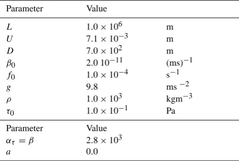
Table 1. Standard values of the parameters for the barotropic
quasi-geostrophic ocean model in the steady flow regime.
Parameter Value
L 1.0×10⁶ m
U 7.1×10⁻³ m
D 7.0×10² m
β0 2.0 10−11 (ms)−1
f0 1.0×10⁻⁴ s−1
g 9.8 ms−2
ρ 1.0×10³ kgm−3
τ0 1.0×10⁻¹ Pa
Parameter Value
ατ =β 2.8×10³
a 0.0
whereej is the j-th unit vector,p∗is the point at which the gradient ofJwith respect topis evaluated andεsmall. The evaluation of the gradient with respect to one parameter re-quires two evaluations of the cost functionJ and in com-parison with the gradient of the cost function with respect to δwdoes not require storage of the Jacobian, nor backward iteration.
4 Results
In this section, we will show the performance of I4D-Var on three test problems using the barotropic ocean model as described in the previous section. The latter model is used as the background model during assimilation and parameter estimation and also for generation of the “observations” of the streamfunctionψ. A standard set of parameter values was chosen that are similar to those in Dijkstra and Katsman (1997) and these values are given in Table 1. With the choice ofUas in Eq. (33) and the wind stress as in Eq. (37a), there are three independent dimensionless parameters in the sys-tem. We fix the value ofβand considerRe,ατandaas our “uncertain” parameters.
Table 2. The values of the dimensionless parameter for each of the
cases I, ..., VI considered.
Regime ατ Re a
I 2800 20 0.0
II 2800 50 0.0
III 2800 120 0.0
IV 2200 20 −0.2
V 3400 50 0.2
VI 3400 120 −0.2
the mid-axis of the basin is broken and no symmetric double gyre solutions exist anymore.
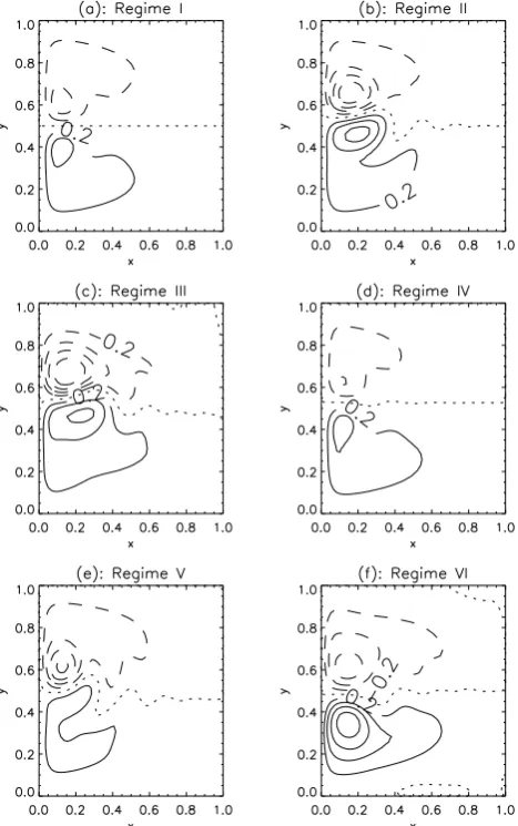
All solutions below are calculated with a time-step of 1 day on an equidistant 60×40 grid. For moderate values of the Reynolds numberRe, this resolution is sufficient to cap-ture an accurate representation of the solutions (Dijkstra and Katsman, 1997). Six different parameter sets were consid-ered to illustrate the capabilities of the I4D-Var method (see Table 2). To show the behavior of the background model in each of these cases, the time evolution of the basin integrated kinetic energy is shown in Fig. 1. For case I, for whicha=0, a steady symmetric state is obtained of which the stream-functionψ is plotted in Fig. 2a. At a slightly larger value ofRe = 50 (case II), an asymmetric steady state (Fig. 2b) is obtained which is a “jet-up” solution. For an even larger value ofRe=120 (case III), the flow is time-dependent and the time-mean of the streamfunction averaged over a 4000 day period is shown in Fig. 2c. For the cases IV, V and VI, the wind-stress forcing is asymmetric (a6=0). While the flows for the cases IV and V approach steady states (shown in Fig. 2d and Fig. 2e, respectively), the flow for case VI is again time-dependent and the time-mean state is plotted in Fig. 2f.
The steady state and time-dependent streamfunction fields were used as the initial background or as synthetic observa-tions in the data-assimilation runs presented below. The ob-servations ofψat all the gridpoints were used, i.e.Hiis equal to the identity operator for alli. Two types of test problems were considered: single-parameter and multi-parameter esti-mation. For multi-parameter estimation, a total of 50 itera-tions were calculated, each with one sequential minimization as described in Sect. 2.3, and we use 6 points per assimilation interval. For the single-parameter estimation runs, the com-putation was terminated after an increase in the optimized cost function was detected at subsequent intervals. For these test problems, 5 point per assimilation interval were used. 4.1 Single parameter estimation
In these test-problems, we useReas the uncertain parame-ter, while the values ofατ anda are fixed. As a first test, the unique steady-steady state solution of case I (Fig. 2a) for Re=20 is taken as the initial background and the synthetic
Fig. 1. Time evolution of the basin integrated kinetic energy for the
different cases I, ..., VI.
observations are derived from the steady-state “jet-up” solu-tion of case II (Fig. 2b) forRe=50.
After a few intervals, the estimate ofRe computed with I4D-Var is already close to “correct” valueRe=50 and even-tually it converges toward this value (Fig. 3a). The value of the cost function for each interval – before minimization over the initial conditions (drawn) and after minimization overRe (dashed) – is shown in Fig. 3b. The value of the cost function converges to zero, indicating that a perfect fit to the synthetic observations is found. For the first interval, the value of the cost function is reduced by about three orders of magnitude after minimization over the initial conditions. In the remain-ing intervals, a decrease of about one order of magnitude is found.
In Fig. 3c, theL2-norm of the differences between the ob-servations and the initial background (drawn) and between the observations and the analysis (dashed) are plotted. The difference between analysis and observations is for all in-tervals smaller than the difference between observations and background and both norms converge to zero indicating that a perfect fit has been found. The difference between the observations and the background increases over the assim-ilation interval which indicates that the background is still attracted away from the observations. However, this effect decreases when the estimate forReapproachesRe=50. Af-ter the first inAf-terval both differences are close to each other at the first point in the second interval. This shows that the model solution at this point is already close to the observa-tions. This is in agreement with the decrease of three orders of magnitude in the cost function as seen in Fig. 3b.
mini-Fig. 2. Contour plots of the streamfunction field: (a) the steady
state of case I; (b) a steady state of case II; (c) a time-mean field of case III; (d) steady state of case IV; (e) a steady state of case V; and
(f) a time-mean field of case VI. The contours are with respect to a
maximum over these 6 fields ofψ=2.25, which is equivalent with a transport of 12.4 Sv (1 Sv=106m3s−1).
mization and after minimization overRe(dashed) are plotted in Fig. 3d. The convergence of the gradient to zero indicates again that both a perfect fit to observations and an accurate estimate ofRehave been found. During the first 14 intervals, the dashed curve is above the dotted curve (Fig. 3d), but the distance between the curves is decreasing and becomes neg-ligibly small after the 14th interval. This indicates that during the first 14 intervals, (large) improvements inReand/or the background model are still possible but that after the 14th interval, the state-parameter solution is very close to the so-lution corresponding to the observations. In summary, for the case in which the initial background and the “observa-tions” are in different dynamical regimes – a unique steady regime (case I) and a multiple equilibria regime (case II) – the performance of I4D-Var is very good.
Fig. 3. Results for initial background from case I and
observa-tions from case II: (a) Re versus the number of intervals (note that the number of intervals is equal to the number of sequen-tial minimizations ofJ); (b) the initial value of the cost function (drawn), its value after minimization over the initial conditions (dot-ted) and after minimization overRe(dashed); (c) theL2-norm of
the difference between the observations and the initial background (drawn) and the difference between the observations and the anal-ysis (dashed); (d) theL2-norm of the initial gradient of the cost
Fig. 4. Results for initial background from case I and observations
from case III: (a)Reversus the number of intervals (note that the number of intervals is equal with the number of sequential mini-mizations ofJ); (b) the initial value of the cost function (drawn), its value after minimization over the initial conditions (dotted) and after minimization overRe(dashed); (c) theL2-norm of the
differ-ences between the observations and the initial background (drawn) and between the observations and the analysis (dashed); (d) theL2
-norm of the initial gradient of the cost function with respect to the increment (drawn), its value after minimization over the initial con-ditions (dotted) and after minimization overRe(dashed).
The second problem to test I4D-Var is slightly more com-plicated as we use the time-dependent observations from case III (Re=120) and as initial background the steady state of
case I (Re=20). As the results in Fig. 4 show, I4D-Var is able to estimate the correct value ofRe(Fig. 4a) and the con-vergence of the different norms is similar (Fig. 4b–d) to that in Fig. 3. This indicates that I4D-Var is also capable of ef-ficiently estimate an uncertain parameter for highly transient observations.
Several other test problems, with other combinations of dynamical behavior – i.e. steady state, periodic, quasi-periodic and irregular, for the initial background and obser-vations – were investigated. The I4D-Var method worked equally well for these problems.
4.2 Multi parameter estimation
Using the barotropic model of the wind-driven circulation, we can also test the performance of I4D-Var in a multi-parameter estimation problem. A maximum of three uncer-tain parameters, Re, ατ and a, can be considered. In all the test problems below, the initial background is the unique steady state of case IV (Fig. 2d). Due to a negative value ofa, this steady state has a small southward jet displacement when compared to the symmetric steady-state of case I (Fig. 2a).
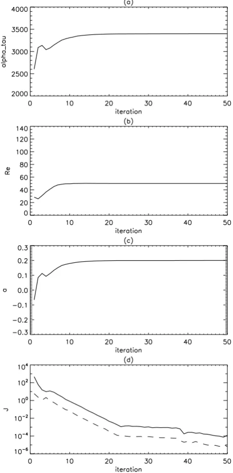
In the first problem, the parameters of case V are estimated by taking its steady-state (Fig. 2e) as the observations. Note that case V has different values for all three parameter than case IV and that, in particular, the value ofa has opposite sign. The steady state in case V is a jet-up solution and hence substantially different than that of case IV (Fig. 2d). Due to the higher value ofατ andRe, the amplitude of the flow is also a lot stronger.
The I4D-Var method is able to find accurate estimates for all parameters. After 10 intervals the estimated values of all three parameters are close to those of case V (Fig. 5a-c). In Fig. 5d, the final value of the cost function after min-imization is one order of magnitude smaller than its value before sequential minimization for all intervals, and two or-ders of magnitude smaller for the first interval. During the first twenty intervals, both values of the cost function rapidly decrease, but after 22 intervals convergence is much slower. This is due to the minimization routine used, which termi-nates when the difference of the cost functionJbetween suc-cessive iterates is smaller than 10−5. After 22 intervals, the initial value of the cost function before minimization over the parameters is smaller than the stop criteria. As a result, the minimization routine will always terminate after one it-eration, which leads to less improvement of the cost function and decrease convergence. This has no consequences for the result. After 20 intervals the final values of the cost function is of order 10−4, and hence the analysis is already sufficiently close to the observations. Furthermore, the estimates for the parameter are accurate after 20 intervals.
Fig. 5. Results for the initial background from case IV and
obser-vations from case V: (a)ατ versus the number of intervals (note
that the number of intervals is equal to the number of sequential minimizations ofJ); (b)Reversus the number of intervals; (c)a
versus the number of intervals; (d) the initial value of the cost func-tion (drawn), its value after minimizafunc-tion over the initial condifunc-tions (dotted) and after minimization overRe(dashed).
solving accurately and efficiently this multi-parameter esti-mation problem.
In the next test problem, we will use the time-dependent streamfunction field of case VI as observations, while still keeping case IV as background. For case VI, the value of Reis even larger than that of case V and the jet oscillates around a “jet-down” mean. Note that one parameter,a, ini-tially has the correct value but that it is free to vary during the parameter estimation procedure.
Fig. 6. Results for initial background from regime IV and
observa-tions from regime VI: (a):ατ versus the number of intervals (note
that the number of intervals is equal with the number of sequen-tial minimizations ofJ); (b)Re versus the number of intervals;
(c)aversus the number of intervals; (d) the initial value of the cost function (drawn), its value after minimization over initial conditions (dotted) and after minimization overRe(dashed).
Fig. 6d and Fig. 5d). The same rapid decrease is seen in the first 20 intervals, as is the slow convergence thereafter due to the stop criteria. The results of this test problem also shows that I4D-Var gives an analysis close to the observations and an accurate estimation of the parameters in the model.
These two test problems were among several investigated. The other problems investigated involved other combinations of several initial steady state solution and their associated pa-rameters and steady state, (quasi-)periodic and irregular ob-servations. For some of these problems one or two parame-ters did have the correct value initially. The result were as good as the two multi-parameter estimation problems dis-cussed in this section. Accurate estimations of the param-eters were found and the analysis was always close to the observations.
5 Conclusions
The main point of this paper was to show that one can per-form 4D-Var data assimilation without using an explicit ad-joint model, when an implicit forward model formulation is available. In that case, the tangent-linear model, needed for the evaluation of the gradient of the cost function, can be de-rived and its transpose can be explicitly calculated without much extra cost.
Implicit forward models have an advantage that usually larger time steps can be taken than with explicit forward models. The choice of the time step in implicit models is not limited by numerical stability, like in explicit models, but by numerical accuracy. The discrete derivation of the im-plicit models is in most cases more complicated than those of explicit models, since the Jacobian matrix has to be ob-tained and large linear systems of equations involving this matrix have to be solved. Over the last decade a hierarchy of implicit ocean and climate models has been developed, aided by the development of efficient solvers for linear systems of equations (Dijkstra, 2000).
Here, a simple one-layer quasi-geostrophic model of the double-gyre wind-driven circulation was used as background model and for generating observations. For this model, the different flow regimes are known for different values of the control parameters. The I4D-Var method performs well in a variety of test problems for this model, involving both single and multi parameter estimation. Even when the initial back-ground model and the observations are chosen in different dynamical regimes, I4D-Var is able to find an accurate esti-mate of the uncertain parameters in the model as well as a perfect fit to the observations.
While this is the first step in the development of implicit 4D-Var methods, there are several issues which need further study to evaluate the potential use of these methods in more realistic models and real world applications. These are (i) the effect of noisy observations and more complex behavior of trajectories, and (ii) the effect of an increase in dimension of the state space. While we cannot address these issues here in depth, we discuss each of them briefly below.
A few additional cases were studied to test the perfor-mance of I4D-Var under “noisy” observations. We added Gaussian noise, with zero mean and a prescribed standard deviationσ, to the model-derived observations and consid-ered a single parameter setup withReas the uncertain pa-rameter. Other parameters had standard values as in Table 1. For the initial background, the symmetric steady state of case I (Re=20) was taken and the observations consisted of the asymmetric steady state from case II (Re=50). For several values ofσ, in the range 0.001−0.2, a twenty-member en-semble of estimations forRewas calculated. The estimates ofRein the ensemble members decreased whenσ was in-creased, but they stabilized between Re=40 and Re=45. However, the spread around the ensemble mean was signifi-cant and the best estimate ofRe(for each values ofσ) was often aroundRe=49. For large standard deviations, the ob-served values ofψclose to zero (right side of the basin and around the jet) can change several orders of magnitude and/or sign. This leads to an ill-posed minimization problem or sud-den increases inJ. Although I4D-Var was not able to esti-mate the value forReexactly, the method is able to provide values close to the correct value.
Variational methods seem to have a disadvantage when compared to the EnKF method, since they rely on accurate adjoints and gradients. In our methodology, we circumvent constructing the adjoint model, by utilizing the extra infor-mation available in the implicit model. In this methodology, we linearize the model at every point of the assimilation in-terval, which gives a gradient that is more accurate than when an adjoint method was used. This makes the estimation tech-nique more suitable for parameter estimation in nonlinear models. In Lea et al. (2000), some fundamental methodolog-ical issues concerning sensitivity analysis of chaotic systems are addressed. They show that, for the Lorenz system, varia-tional methods are a limited tool for sensitivity analysis and parameter estimation, due to the behavior of the adjoint and gradient for various time scales. Note that Lea et al. (2000), however, also found a range of time-scales for which the ad-joint was reasonably accurate. This suggests that if the in-tegration segment is chosen carefully, variational methods, such as I4D-Var, may still produce good results.
atmo-sphere models with reasonable resolution. The main advan-tage of I4D-Var over traditional 4D-Var methods is that at each time step, changes in the state due to a parameter vari-ation are taken into account because of the availability and use of the local Jacobian matrix.
In summary, the results look promising and motivating enough to apply I4D-Var to problems where the dimension of the state space is much larger and where “real” (noisy) observations are used.
Acknowledgements. The authors thank the organizers of the
session “Nonlinear Dynamics of Earth, Oceans and Space” at the first AOGS meeting in Singapore (July 2004), F. Wubs and A. de Niet (both University of Groningen, the Netherlands) for the ongoing collaboration, and an anonymous reviewer for very thoughtful comments on the first version of this paper. This work was supported by the Dutch Technology Foundation (STW) within the project GWI.5798.
Edited by: P. C. Chu Reviewed by: one referee
References
Anderson, J.: An ensemble adjustment Kalman filter for data as-similation, Monthly Weather Review, 129, 2884–2902, 2001. Annan, J. and Hargreaves, J.: Efficient parameter estimation for a
highly chaotic system, Tellus, 56A, 520–526, 2004.
Annan, J., Hargreaves, J., Edwards, N., and Marsh, R.: Parameter estimation in an intermediate complexity earth system model us-ing an ensemble Kalman filter, Ocean Modellus-ing, 8, 135–154, 2005.
Botta, E. F. F. and Wubs, F. W.: MRILU: An effective algebraic multi-level ILU-preconditioner for sparse matrices, SIAM J. Ma-trix Anal. Appl., 20, 1007–1026, 1999.
Courtier, P., Th´epaut, F.-N., and Hollingsworth, A.: A strategy for operational implementation of 4D-Var, using an incremental ap-proach, Quart. J. Roy. Meteor. Soc., 120, 1367–1388, 1994. Derber, J.: A variational continuous assimilation method, Monthly
Weather Review, 117, 2437–2446, 1989.
Dijkstra, H. A.: Nonlinear Physical Oceanography: A Dynami-cal Systems Approach to the Large SDynami-cale Ocean Circulation and El Ni˜no., Kluwer Academic Publishers, Dordrecht, The Nether-lands, 2000.
Dijkstra, H. A. and Katsman, C. A.: Temporal variability of the Wind-Driven Quasi-geostrophic Double Gyre Ocean Circula-tion: Basic Bifurcation Diagrams, Geophys. Astrophys. Fluid Dyn., 85, 195–232, 1997.
Evensen, G.: Sequential data assimilation with a non-linear quasi-geostrophic model using Monte-Carlo methods to forecast error statistics, J. Geophys. Res., 53, 10 143–10 162, 1994.
Evensen, G.: The ensemble Kalman filter: theoretical formulation and practical implementation, Ocean Dynamics, 53, 343–367, 2003.
Hargreaves, J., Annan, J., Edwards, N., and Marsh, R.: An effi-cient climate forecasting method using an intermediate complex-ity Earth System Model and the ensemble Kalman filter, Climate Dynamics, 23, 745–760, 2004.
Kalman, R.: A new approach to linear filtering and prediction prob-lems, J. Basic Eng., 82D, 33–45, 1960.
Klinker, E., Rabier, F., Kelly, G., and Mahfouf, J.-F.: The ECMWF operational implementation of four dimensional variational as-similation, Part III: Experimental results and diagnostics with op-erational configuration, Quart. J. Roy. Meteor. Soc., 126, 1191– 1215, 2000.
Lea, D., Allen, M., and Haine, T.: Sensitivity analysis of the climate of a chaotic system, Tellus, 52A, 523–532, 2000.
Lorenz, E. N.: Deterministic nonperiodic flow., J. Atmos. Sci., 20, 130–141, 1963.
Mahfouf, J.-F. and Rabier, F.: The ECMWF operational implemen-tation of four dimensional variational assimilation. Part II: Ex-perimental results with improved physics, Quart. J. Roy. Meteor. Soc., 126, 1171–1190, 2000.
Nash, S. and Sofer, A.: Linear and nonlinear programming, McGraw-Hill series on industrial and management sciences, McGraw-Hill, 1996.
Navon, I.: Practical and theoretic aspects of adjoint parameter es-timation and identifiability in meteorology and oceanography, Dyn. Atmos. Oceans, 27, 55–79, 1998.
Pedlosky, J.: Geophysical Fluid Dynamics. 2nd Edn, Springer-Verlag, New York, 1987.
Rabier, F., J¨arvinen, H., Klinker, E., Mahfouf, J.-F., and Simmons, A.: The ECMWF operational implementation of four dimen-sional variational assimilation. Part I: Experimental results with simplified physics, Quart. J. Roy. Meteor. Soc., 126, 1143–1170, 2000.
Vialard, J., Weaver, A., Anderson, D., and Delecluse, P.: Three- and four-dimensional variational assimilation with an ocean general circulation model of the tropical Pacific. Part II: physical valida-tion, Monthly Weather Review, 131, 1379–1395, 2003. Weaver, A., Vialard, J., Anderson, D., and Delecluse, P.: Three- and
four-dimensional variational assimilation with an ocean general circulation model of the tropical Pacific., Part I: formulation, in-ternal diagnostics and consistency checks, Monthly Weather Re-view, 131, 1360–1378, 2003.
Weijer, W., Dijkstra, H. A., Oksuzoglu, H., Wubs, F. W., and De Niet, A. C.: A fully-implicit model of the global ocean circu-lation, J. Comp. Phys., 192, 452–470, 2003.
Yu, L. and O’Brien, J.: Variatational estimation of the wind stress drag coefficient and the oceanic eddy viscosity profile, J. Phys. Oceanogr., 21, 709–719, 1991.