Nonlinear Processes in Geophysics Exact theory for localized envelope modulated electrostatic wavepackets in space and dusty plasmas

SRef-ID: 1607-7946/npg/2005-12-407 European Geosciences Union

© 2005 Author(s). This work is licensed under a Creative Commons License.

Nonlinear Processes

in Geophysics

Exact theory for localized envelope modulated electrostatic

wavepackets in space and dusty plasmas

I. Kourakis1, 2and P. K. Shukla1

1_{Institut f¨ur Theoretische Physik IV, Fakult¨at f¨ur Physik und Astronomie, Ruhr-Universit¨at Bochum, D-44780 Bochum,}

Germany

2_{Max-Planck-Institut f¨ur extraterrestrische Physik, Giessenbachstrasse, D-85740 Garching, Germany}

Received: 2 November 2004 – Accepted: 25 January 2005 – Published: 18 March 2005 Part of Special Issue “Nonlinear plasma waves-solitons, periodic waves and oscillations”

Abstract. Abundant evidence for the occurrence of

mod-ulated envelope plasma wave packets is provided by recent satellite missions. These excitations are characterized by a slowly varying localized envelope structure, embedding the fast carrier wave, which appears to be the result of strong modulation of the wave amplitude. This modulation may be due to parametric interactions between different modes or, simply, to the nonlinear (self-)interaction of the carrier wave. A generic exact theory is presented in this study, for the nonlinear self-modulation of known electrostatic plasma modes, by employing a collisionless fluid model. Both cold (zero-temperature) and warm fluid descriptions are discussed and the results are compared. The (moderately) nonlinear os-cillation regime is investigated by applying a multiple scale technique. The calculation leads to a Nonlinear Schr¨odinger-type Equation (NLSE), which describes the evolution of the slowly varying wave amplitude in time and space. The NLSE admits localized envelope (solitary wave) solutions of bright-(pulses) or dark- (holes, voids) type, whose characteristics (maximum amplitude, width) depend on intrinsic plasma pa-rameters. Effects like amplitude perturbation obliqueness (with respect to the propagation direction), finite tempera-ture and defect (dust) concentration are explicitly consid-ered. Relevance with similar highly localized modulated wave structures observed during recent satellite missions is discussed.

1 Introduction

In a wide variety of physical contexts, the dynamics of prop-agating periodic excitations (waves) is dominated by a com-petition between the effects of “mode dispersion” and “non-linearity” of the medium. The latter mechanism, which is ig-nored when studying harmonic (linear) wave propagation in the small-amplitude limit, generally increases when the

dis-Correspondence to: I. Kourakis

([email protected])

placement from equilibrium grows bigger. For a sufficiently important excitation amplitude, it is known that nonlinearity may be strong enough to balance spatial delocalization (i.e. mode separation due to dispersion) and thus result to the for-mation of propagating localized structures (solitary waves, solitons). On the other hand, weakly nonlinear effects enter into play as the wave amplitude acquires (even small yet) fi-nite (non negligible) values, moderately beyond the linear ap-proximation. The generic signature of this mechanism is the appearance of secondary phase “harmonics” in the Fourier spectrum of the system observed, in addition to a nonlinear modulation of the wave’s amplitude, manifested as a slow variation of the wave’s amplitude in space and time. The oc-currence of amplitude modulation may be due to parametric wave coupling, interaction between high- and low- frequency modes or, simply, self-interaction of the carrier wave (“auto”-or “self”-modulation). Furtherm(“auto”-ore, analytical and numeri-cal studies have established the relevance of these phenom-ena with modulational instability, which may lead to energy localization via localized pulse formation, as known in fields as diverse as Nonlinear Optics, Condensed Matter Physics and Biophysics (Davydov, 1985; Hasegawa, 1989; Infeld, 1990; Remoissenet, 1994).

Charged matter (plasma), a nonlinear and dispersive medium “par excellence”, provides a typical paradigm for the study of such mechanisms. As far as plasma modes are concerned (Krall and Trivelpiece, 1973; Stix, 1992), the oc-currence of such phenomena has been confirmed by exper-iments related to the nonlinear propagation of electrostatic (ES, e.g. ion-acoustic) (Watanabe 1977; Bailung and mura, 1993; Luo et al., 1998; Nakamura et al., 1999; Naka-mura and Sarma, 2001) as well as electromagnetic (EM, e.g. whistler) waves (Kostrov, 2003). Recent numerical simu-lations of electron cyclotron waves (Eliasson and Shukla, 2004) (as well as earlier ones, by Hasegawa, 1970, 1972) also predict such a behaviour.

408 I. Kourakis and P. K. Shukla: Localized envelope modulated electrostatic wavepackets

Figures

Fig. 1. Modulated structures, related to ‘chorus’ (EM) emission in the magnetosphere [CLUSTER satellite

data; reprinted from (Santolik, 2003)].

Fig. 2. Electrostatic noise wave forms, related to modulated electron-acoustic waves [FAST satellite data; figure

reprinted from (Pottelette et al., 1999)]. The co-existence of a high (carrier) and a low (modulated envelope) frequencies is clearly reflected in the Fourier spectrum, in the right.

Fig. 3. Localized envelope structures in the magnetosphere [reprinted from (Alpert, 2001)].

31

Fig. 1. Modulated structures, related to “chorus” (EM) emission in the magnetosphere (CLUSTER satellite data; reprinted from Santo-lik, 2003).

Ergun et al., 1998a, 1998b; Pottelette et al., 1999), as well as the S3-3 (Temerin, 1982), Viking (Bostr¨om, 1988), GEO-TAIL and POLAR earlier missions in the magnetosphere (Matsumoto et al., 1994; Franz et al., 1998; Cattell et al., 1999, 2003; McFadden et al., 2003) (also see many ref-erences therein) (the interpretation of the Viking measure-ments, Bostrom, 1988, has recently risen some doubt; see the thorough discussion in McFadden et al., 2003). Some of the localized structures reported therein bear qualitative characteristics which are reminiscent of solitary electrostatic waves and are strongly believed to be related to ion acous-tic waves; see the discussion in (McFadden et al., 2003). It should be stressed that both compressive and rarefactive large amplitude structures have been observed (Matsumoto et al., 1994; Franz et al., 1998; Cattell et al., 1999, 2003) (also see many references therein). Note that it was recently suggested by McFadden et al. (2003) that neither the veloc-ity dependence of the observed potential structure amplitudes nor their asymmetry should be taken for granted, since they may be attributed to intrinsic measurement errors. Finally, the observed phase speeds lie over an extended region of values, sometimes even above the ion sound velocity; these facts seem to suggest that plainly employing the soliton (Ko-rteweg – deVries, KdV) picture may not suffice for the elu-cidation of the generation of these solitary structures and an alternative instability mechanism may be present; also see the discussion in (Berthomier et al., 1998; McFadden et al., 2003). Localized modulated wave packets, in particular, are encountered in abundance e.g. in the Earth’s magnetosphere, where they are associated with localized field and/or density variations simultaneously observed (Pottelette et al., 1999; Alpert, 2001; Santolik, 2003). The occurrence of such wave forms is, for instance, thought to be related to the broadband electrostatic noise (BEN) encountered in the “auroral” region (Pottelette et al., 1999).

Recent analytical studies have supplied evidence for the relevance of nonlinear modulational effects in dust-contaminated plasmas (“Dusty” or “Complex” Plasmas), where a strong presence of mesoscopic, massive, charged dust grains strongly affects the characteristics of the plasma (Verheest, 2001; Shukla and Mamun, 2002). The modifica-tion of the plasma response due to the presence of dust gives rise to new ES/EM modes, whose self-modulation was re-cently shown to lead to modulational instability and soliton formation; these include e.g. the dust-acoustic (DA) (Rao et al., 1990; Amin et al., 1998; Tang and Xue, 2003; Kourakis

Fig. 1. Modulated structures, related to ‘chorus’ (EM) emission in the magnetosphere [CLUSTER satellite

data; reprinted from (Santolik, 2003)].

Fig. 2. Electrostatic noise wave forms, related to modulated electron-acoustic waves [FAST satellite data; figure

reprinted from (Pottelette et al., 1999)]. The co-existence of a high (carrier) and a low (modulated envelope) frequencies is clearly reflected in the Fourier spectrum, in the right.

Fig. 3. Localized envelope structures in the magnetosphere [reprinted from (Alpert, 2001)].

31

Fig. 2. Electrostatic noise wave forms, related to modulated electron-acoustic waves (FAST satellite data; figure reprinted from Pottelette et al., 1999). The co-existence of a high (carrier) and a low (modulated envelope) frequencies is clearly reflected in the Fourier spectrum, in the right.

and Shukla, 2004a) and dust-ion acoustic (DIA) ES modes (Shukla and Silin, 1992; Amin et al., 1998; Kourakis and Shukla, 2003a, 2004b), in addition to magnetized plasma modes, e.g. the Rao EM dust mode (Kourakis and Shukla, 2004c).

The purpose of this paper is to provide a “generic” methodological framework for the study of the nonlinear (self-) modulation of the amplitude of electrostatic (ES) plasma modes. The results which follow cover a variety of ES modes. We mean to emphasize the generic character of the nonlinear behaviour of these modes, so focusing upon a specific mode is avoided on purpose. Where appropriate, de-tails regarding specific modes may be sought in (Kourakis and Shukla, 2003a, b, 2004a, b, d), where some of this mate-rial was first presented.

In the following, we study the modulational instability of electrostatic plasma waves propagating “along” the magnetic field, so that the Lorentz forces can be omitted. Amplitude modulation is allowed to take place in an oblique direction, at an angle θ with respect to the carrier wave propagation direction. By assuming the wave’s amplitude to vary on slow space and time scales, sayXandT (see definitions be-low), we shall seek an evolution equation for the amplitude

ψ (X, T ), establish its oscillatory solution and then establish an explicit criterion for modulational (in)stability. Our aim is to trace the influence ofθ on the conditions for modula-tional instability onset, and determine the magnitude of the associated instability growth rate. We shall also examine the possibility of the formation of localized excitations and dis-cuss their characteristics. Exact new expressions are derived for quantities of interest, in terms of the system’s dispersion laws and the intrinsic plasma parameters.

I. Kourakis and P. K. Shukla: Localized envelope modulated electrostatic wavepackets 409

Fig. 1. Modulated structures, related to ‘chorus’ (EM) emission in the magnetosphere [CLUSTER satellite

data; reprinted from (Santolik, 2003)].

Fig. 2. Electrostatic noise wave forms, related to modulated electron-acoustic waves [FAST satellite data; figure

reprinted from (Pottelette et al., 1999)]. The co-existence of a high (carrier) and a low (modulated envelope) frequencies is clearly reflected in the Fourier spectrum, in the right.

Fig. 3. Localized envelope structures in the magnetosphere [reprinted from (Alpert, 2001)].

31

Fig. 3. Localized envelope structures in the magnetosphere reprinted from Alpert (2001).

and space. The exact form of dispersion and nonlinearity coefficients in the NLS-type equation is presented and dis-cussed. In Sect. 4, we carry out a stability analysis of the NLSE allowing for a thorough study of the DA wave stabil-ity in various regions of the physical parameters involved. We pursue the analysis in Sect. 5, by discussing the possibil-ity of the existence of localized solutions of the NLSE, and identifying their forms in different parameter regions. The relevance of the formalism with known plasma modes is dis-cussed in Sect. 6. Finally, our results are briefly disdis-cussed and summarized in the concluding Sect. 7.

2 The model: formulation and analysis

In a general manner, several known electrostatic plasma modes (Stix, 1992; Swanson, 2003) are adequately described by (single) fluid models; ES plasma modes are thus as-sociated with propagating oscillations which are related to “one” dynamical plasma constituent, sayα(massmα, charge

qα ≡sαZαe; eis the absolute electron charge; s =sα =

qα/|qα| = ±1 is the charge “sign”), against a background of one (or more) constituent(s), sayα0(massmα0, chargeq_α0 ≡

sα0Z_α0e, similarly). The background species is (are) often

as-sumed to obey a known distribution, e.g. to be in a fixed (uni-form) or in a thermalized (Maxwellian) state, for simplicity, depending on the particular aspects (e.g. frequency scales) of the physical system considered. For instance, the “ion-acoustic” (IA) mode refers to ions (α=i) oscillating against a (much hotter) electron background (α0=e), which may be considered to be Maxwellian (Krall and Trivelpiece, 1973; Kourakis and Shukla, 2003b); the “electron-acoustic” (EA) mode (Krall and Trivelpiece, 1973; Kourakis and Shukla, 2004d) can be modelled as electron oscillations (α = e) against a background of ions (α0 =i), which are practically immobile (fixed), and so forth (Krall and Trivelpiece, 1973; Stix, 1992). The coexistence of “hot” (h) and “cold” (c) elec-tron populations, observed in the upper parts of the Earth’s magnetosphere (Berthomier et al., 1998), may also readily be accommodated in this description, in order to study its influence on IA (α = i,α0 = c, h) (Kourakis and Shukla, 2003b) and EA (α = c,α0 = i, h) (Kourakis and Shukla, 2004d) waves. As regards “dusty plasma” modes, the DA mode describes oscillations of dust grains (α=d) against a Maxwellian electron and ion background (α0=e, i) (Shukla and Mamun, 2002; Kourakis and Shukla, 2004a), while DIA waves denote IA oscillations in the presence of inertial dust

in the background (α=i,α0 =e, d) (Shukla and Mamun, 2002; Kourakis and Shukla, 2003a; Kourakis and Shukla, 2004b).

2.1 A generic fluid description

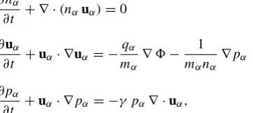
A standard (single) fluid model to be employed for the dy-namic speciesαconsists of the first moment evolution equa-tions, namely the density nα (conservation) equation, the mean fluid velocity equation and the pressure equation:

∂nα

∂t + ∇ ·(nαuα)=0 ∂uα

∂t +uα· ∇uα = − qα

mα

∇8− 1

mαnα ∇pα

∂pα

∂t +uα· ∇pα = −γ pα∇ ·uα, (1)

where nα, uα and pα respectively denote the “density”, “mean” (fluid) “velocity” and “pressure” of speciesα. The parameter γ = cP/cV = 1 +2/f denotes the specific heat ratio (for f degrees of freedom), e.g. γ = 3 in the one-dimensional (“1d”) case,γ =2 in the two-dimensional (“2d”) andγ = 5/3 in the three-dimensional (“3d”) case; also,γ =1 if an adiabatic evolution is considered.

The electric potential8obeys Poisson’s eq.: ∇28 = −4π X

α00_=α,{α0_}

qα00n_α00 = 4π e (n_e−Z_in_i+...) ,(2)

where all the particle species appear in the right-hand side (“rhs”). Overall charge neutrality is assumed at equilibrium, i.e.

qαnα,0= −

X

α0

qα0n_α0_,0. (3)

2.2 Reduced description

By choosing appropriate scales for all quantities, the above system of evolution equations may be cast into the following form:

∂n

∂t + ∇ ·(nu)=0, (4)

∂u

∂t +u· ∇u= −s∇φ− σ

n∇p, (5)

∂p

∂t +u· ∇p= −γ p∇ ·u (6)

(the indexαwill be understood where omitted, viz.s=sα). The re-scaled (dimensionless) dynamic variables are now:

n = nα/nα,0, u = uα/c∗, p = pα/(nα,0kBTα), and

φ = |qα|8/(kBT∗), where nα,0 is the equilibrium density

andc∗ =(kBT∗/mα)1/2is a characteristic (e.g. sound) ve-locity. Time and space are scaled over appropriately chosen scalest0 (e.g.ω−_p,α1 = (4π nα,0qα2/mα)−1/2) andr0 =c∗t0;

p0=nα,0kBTα), andT∗is an effective temperature (related

to the background considered), to be determined for each problem under consideration (kB is Boltzmann’s constant). The temperature ratioTα/T∗is denoted byσ, in this “warm

model” (Chan and Seshadri, 1975; Durrani et al., 1979) (the so-called “cold model” is recovered for σ = 0; see that Eq. (6) then becomes obsolete). The Lorentz force term was omitted, since wave propagation along the external magnetic field is considered here. The system is closed by Poisson’s equation, which may now be expressed as1

∇2φ = −sn +X α0

nα0q_α0/(n_α,0q_α) ≡ −s (n− ˆn) . (7)

Note that the neutralizing background (reduced) density ˆ

n= −X α0

nα0q_α0

nα,0qα

= − 1

sαZαnα,0

X

α0

sα0Z_α0n_α0 (8)

is a priori2 a function of the potentialφ (note thatnˆ = 1 forφ =0, due to the equilibrium neutrality condition); fur-thermore, it depends on the physical parameters (e.g. back-ground temperature, plasma density, defect concentration, ...) involved in a given problem. The calculation in the specific case of IA waves is explicitly provided below, for clarity. 2.3 Weakly nonlinear oscillation regime

What follows is essentially an implementation of the long known “reductive perturbation” technique (Taniuti and Ya-jima, 1969; Asano et al., 1969; Shimizu and Ichikawa, 1972; Kako, 1974; Kakutani, 1974), which was first applied in the study of electron plasma (Taniuti and Yajima, 1969; Asano et al., 1969) and electron-cyclotron (Hasegawa 1970, 1972) waves, more than three decades ago.

Equations (4)–(7) describe the evolution of the state vec-tor3 S = {n,u, p, φ}which accepts a harmonic (electro-static) wave solution in the form S=S0exp[i(kr−ωt)] +

c.c., in the weak amplitude approximation, i.e. forS0,j 1. Once the amplitude of this wave becomes non-negligible, a nonlinear harmonic generation mechanism enters into play: this is the first signature of nonlinearity, which manifests its presence once a slight departure from the weak-amplitude (linear) domain occurs. In order to study the nonlinear (am-plitude) modulational stability profile of these electrostatic waves, we consider small deviations from the equilibrium state S(0)_=(1,0,1,0)T_{, viz. S=S}(0)_+S(1)₊2_S(2)_+..., where 1 is a smallness parameter. We have as-sumed that4S_j(n) = P∞

l=−∞ S (n)

j,l(X, T )exp[il(kr−ωt)]

1_{A factorω}2

p,αt02 is omitted in the right-hand side of Eq. (7),

since equal to 1 fort0=ω−p,α1.

2_{This is only not true when the background is assumed fixed,}

e.g. for EA waves (i.e.sα = −sα0 = −1, n_α0 = n_i = const.),

wherenˆ=Z_in_i/n_e,0=const.

3_{Note that S ∈ <}d+3 _{in a d− dimensional problem (d =}

1,2,3).

4_{In practice, only terms withl≤ndo contribute in this}

summa-tion. This simply means that up to 1st harmonics are expected for n=1, up to 2nd phase harmonics forn=2, and so forth.

(for j = 1,2, ..., d + 3; see footnote 3; the condition

S_j,(n)_−l = S_j,l(n)∗ holds, for reality). The wave amplitude is thus allowed to depend on the stretched (“slow”) coordinates

X = (x−λ) tandT = 2t; the real variableλ, to be de-termined, will later be interpreted as the wave’s “group veloc-ity” along the modulation directionx. The amplitude mod-ulation direction (∼ ˆx) is assumed “oblique” with respect to the (arbitrary) propagation direction, which is expressed by the wave vectork = (kx, ky) = (kcosθ, ksinθ ); cf. (Kako and Hasegawa, 1976; Chhabra and Sharma, 1986; Mishra et al., 1994), where a similar treatment is adopted. Note that (not having taken the magnetic field into account in the analysis) this is essentially a “2d” physical problem, although readily applicable in a three-dimensional (“3d”) de-scription, for completeness. We shall limit ourselves to con-sidering two axes (xandy) in the following.

According to the above considerations, we set:

∂/∂t→∂/∂t− λ ∂/∂X+2∂/∂T ,

∂/∂x→∂/∂x+ ∂/∂X ,

(while∂/∂yremains unchanged) and ∇2→ ∇2+2 ∂2/∂x∂X+2∂2/∂X2,

so that

∂ ∂t A

(n) l e

ilθ1 ₌

−ilω A(n)_l − λ∂A

(n) l

∂X + 2∂A

(n) l

∂T

×eilθ1_, ∇A(n)_l eilθ1 ₌

ilkA(n)_l +xˆ∂A (n) l

∂X

eilθ1_,

∇2A(n)_l eilθ1 ₌

−l2k2A(n)_l +2 ilkx

∂A(n)_l ∂X

+2∂ 2_A(n)

l

∂X2

eilθ1 ₍₉₎

for anyl−th phase harmonic amplitudeA(n)_l among the com-ponents of S(n)_l ; obviously, θ1 here denotes the elementary phaseθ1≡kr−ωt.

By expanding nearφ≈0, Poisson’s eq. may formally be cast in the form

∇2φ = φ−α φ2+α0φ3−s β (n−1) , (10) where the exact form of the real coefficientsα,α0andβ (to be distinguished from the species indices above, obviously) are to be determined exactly for any specific problem, and contain all the essential dependence on the plasma param-eters. Note that the right-hand side in Eq. (10) cancels at equilibrium.

2.4 A case study: ion-acoustic waves

In order to make our method and notation concise and clear, let us explicitly consider the simple case of “ions” (thusα=

iandqα = qi = +Zie, i.e.sα = +1) oscillating against thermalized “electrons” (viz. α0 = eandqα0 = q_e = −e,

i.e.sα0 = −1; n_e = n_e,0ee8/(kBTe)). Adopting the scaling

defined above, and using the equilibrium neutrality condition

ne,0=Zini,0, it is a trivial exercise to cast Poisson’s Eq. (2)

into the (reduced) form:

∇2φ= −(ωp,ir0/c∗)2[n−eT∗φ/(ZiTe)] ≡ −(n−eξ φ) ,

where we took: t0 = r0/c∗ = ω_p,i−1 andξ ≡ T∗/(ZiTe). Now, expanding nearφ≈0, viz.eξ φ≈1+ξ φ+ξ2φ2/2+

ξ3φ3/6+..., we have:

∇2φ≈ξ φ+ξ2φ2/2+ξ3φ3/6−(n−1) .

Finally, setting the temperature scaleT∗equal toT∗=ZiTe, for convenience (so that ξ = 1)5_{, one recovers exactly}

Eq. (10) withα= −1/2,α0=1/6 andβ=1.

The amplitude modulation of ion-acoustic waves was first studied for parallel modulation (i.e. in the direction of propa-gation, viz.θ =0) in (Shimizu and Ichikawa, 1972), and for oblique modulation in (Kako and Hasegawa, 1976); as ex-pected, those results are recovered from the formulae below.

3 Perturbative analysis

By substituting the perturbative series defined in the previ-ous Section into Eqs. (4)–(6) and (10) and isolating distinct orders in, we obtain a set of reduced equations for the har-monic amplitude at each (nth-) order. Solving at each order and substituting in th following one, one successively obtains a linear homogeneous (Cramer-type) system of equations, whose solution provides the amplitudes of thel−th harmonic contributions at order n (i.e. n(n)_l , u_x/y,l(n) , p_l(n), φ_l(n), viz.

l = 0,1,2, ..., n for every n = 1,2,3, ...). The compati-bility condition obtained at each order, appearing e.g. as the requirement of a determinant to be equal to zero, need also be taken into account.

The details of the tedious calculation are explicitly pro-vided in the Appendix, so only a few essential steps are ex-posed in the following, for clarity.

3.1 1st-order quantities – dispersion relation

The first harmonic amplitudes are determined (to order∼1) as

n(₁1) = s1+k 2

β ψ =

k ωcosθu

(1)

1,x =

k ωsinθu

(1)

1,y =

p₁(1) γ (11) 5_{Note that a different choice forT}

∗would lead to a modified

right-hand-side in Eq. (10), i.e. a factorξ 6= 1 would precede the first term (inφ). This might, of course, also be a legitimate choice of scaling; however, the following formula are not valid – and should be appropriately modified – in this case. Obviously though, the qualitative results of this study are not affected by the choice of scaling.

in terms e.g. of the potential correctionφ₁(1)≡ψ, along with the dispersion relation

ω2 = βk

2

k2₊₁ +γ σ k

2_{. (12)}

See that the expected acoustic behaviourω ∼kis obtained for low wavelengths, i.e. fork1.

3.2 2nd-order quantities - group velocity

The amplitudes of the 2nd and 0th (constant) harmonic cor-rections are obtained in order∼2(the lengthy expressions can be found in the Appendix); retain that the former (later) are proportional toψ2(|ψ|2, respectively).

The compatibility condition obtained forn=2 andl =1 provides exactly the constraint:

λ= ∂ω(k)

∂kx

≡vg, (13)

suggesting that the parameterλ denotes the velocity vg at which the wave’s amplitude travels along the modulation di-rectionx; for parallel modulation (viz.θ =0) this is simply the “group velocity”∂ω(k)/∂k6; see Eq. (A12) in the Ap-pendix for the exact expression forvg.

3.3 3rd-order quantities - the envelope evolution equation At this stage, one has obtained a solution up to second order, viz.

n≈n0+{n(₁1) exp[i(kr−ωt )] +c.c.}

+2

n(₀2) + {n(₂2) exp[2i(kr−ωt )] +c.c.}

+O(3)

for the density (see that we have takenn(₁2)=0, with no loss of generality), along with analogous expressions for the other state variables, namely velocity componentsux/y, pressurep and potentialφ.

Isolating the evolution equations for n = 3 and l = 1, one obtains an explicit condition for suppression of “secular terms” to be obeyed by the potential correctionψ, i.e. a com-patibility condition in the form of a “nonlinear Schr¨odinger– type equation” (NLSE)

i∂ψ ∂T +P

∂2ψ

∂X2+Q|ψ|

2_{ψ=0. (14)}

6_{This is a – physically expected – constraint which is imposed}

by the equations forn = 2 andl = 1 (1st harmonics at 2nd or-der). Alternatively, one may assume a dependence onXn = nx (plus a similar expansion fory, zandt) forn = 0,1,2, ...; the condition for annihilation of secular terms then reads:∂A(₁1)/∂T1+

(∂ω/∂kx)∂A(₁1)/∂X1, i.e.A(₁1)=A(₁1)(X1−vgT1)(for any of the

-40 -20 20 40

-1 -0.5 0.5 1

(a)

-20 -10 10 20

-0.4 -0.2 0.2 0.4 0.6 0.8 1

(b)

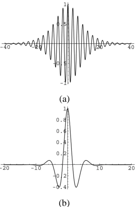
Fig. 4. Bright type modulated wavepackets (for

P Q >

0

), for two different (arbitrary) sets of parameter values.

32

Fig. 4. “Bright” type modulated wavepackets (forP Q > 0), for two different (arbitrary) sets of parameter values.

The “dispersion coefficient”P is in fact related to the cur-vature of the dispersion curve as

P = 1 2

∂2ω ∂k2

x = 1

2

ω00(k)cos2θ + ω 0_(k)

k sin 2_θ

(15) (the prime denotes differentiation); see that the expected de-pendenceP =∂2ω/2∂k2, which is familiar from nonlinear optics (Hasegawa, 1989) is obtained for θ = 0. The full expression forP is given by Eq. (A20) in the Appendix.

The “nonlinearity coefficient”Q, which is due to the car-rier wave self-interaction, is given by a lengthy expression, reported in the Appendix.

Both coefficientsP andQ are functions of k, θ and β

(in addition toα, α0, forQ), as expected. The exact general expressions obtained (see in the Appendix) may be “tailor fit” to any given electrostatic plasma wave problem (via the form of the parametersα, α0, β), in view of a numerical in-vestigation of the wave’s amplitude dynamics (e.g. stability profile, wave localization; see in the following). One thus obtains the (tedious) analytical form ofP andQin terms of intrinsic plasma parameters such as background plasma den-sity, temperature, defect concentration, background species

composition (if more than one species is present in the back-ground), and so forth. Also note the approximate expressions obtained in the end of the Appendix, which are valid for large wavelength (i.e. small wavenumber) values.

4 Modulational (in)stability analysis

It is known (see e.g. in Hasegawa, 1975, 1989; Remoissenet, 1994) that the evolution of a wave whose amplitude obeys Eq. (14) depends on the coefficient productP Q, which may be investigated in terms of the physical parameters involved. To see this, first check that Eq. (14) supports the plane (Stokes’) wave solutionψ = ψ0exp(iQ|ψ0|2T ); the stan-dard linear analysis consists in perturbing the amplitude by setting:ψˆ = ˆψ0 +ψˆ1,0cos(kX˜ − ˜ωT )(the perturbation

wavenumberkˆ and the frequencyωˆ should be distinguished from their carrier wave homologue quantities, denoted byk

andω). One thus obtains the (perturbation) dispersion rela-tion:

˜

ω2 = P k˜2(Pk˜2 −2Q| ˆψ1,0|2) . (16)

One immediately sees that ifP Q > 0, the amplitudeψ is “unstable” fork <˜ √2Q/P| ˆψ1,0|; i.e. for perturbation

wave-lengths larger than a critical value. IfP Q < 0, the ampli-tudeψwill be “stable” to external perturbations. This “mod-ulational instability” mechanism is tantamount to the well-known “Benjamin-Feir” instability, in hydrodynamics, also long-known as an energy localization mechanism in solid state physics and nonlinear optics (Hasegawa, 1989; Infeld, 1990; Remoissenet, 1994).

This type of analysis allows for a numerical investiga-tion of the stability profile in terms of parameters e.g. like wavenumberk, perturbation (obliqueness) angleα, temper-atureTα, background plasma parameters etc. A few known ES modes have already thus been investigated; see in Sect. 6 below.

5 Envelope excitations

It should be pointed out that the evolution Eq. (14) is known to be integrable (Infeld, 1990; Remoissenet, 1994). Its lo-calized solutions, which can be rigorously obtained via the tedious Inverse Scattering Transform method, are properly speaking “solitons”, in the sense that they satisfy an infin-ity of conservation laws; they have been shown analytically (and confirmed numerically) to survive collisions between one another and also exhibit a robust behaviour against ex-ternal perturbations.

The modulated (electrostatic potential) wave finally result-ing from the above analysis is of the form7

φ(₁1)=ψ0ˆ cos(kr−ωt+2)+O(2).

7_{In fact, the potential correction amplitude here isψ}ˆ

0 = 2ψ0,

Note that once the potential correction φ₁(1) is determined, density, velocity and pressure corrections follow from Eq. (11). The slowly varying amplitudeψ0(X, T )and phase correction2(X, T ) (both real functions of {X, T}; see in Fedele and Schamel, 2002a; Fedele et al., 2002b for details) are determined by (solving) Eq. (14) for

ψ=ψ0exp(i2).

The different types of solution thus obtained are summarized in the following.

5.1 Bright-type envelope solitons

For “positive”P Q, the carrier wave is modulationally “un-stable”; it may either “collapse”, due to (possibly random) external perturbations, or lead to the formation of “bright” envelope modulated wavepackets, i.e. localized envelope “pulses” confining the carrier (see Fig. 4), given by (Fedele and Schamel, 2002a; Fedele et al., 2002b)8

ψ0=

˜

ψ0

1/2

sech

_X−v

eT

L

,

2= 1 2P

veX+

−v

2

e 2

T

, (17)

where ve is the envelope velocity; L and represent the pulse’s spatial width and oscillation frequency (at rest), respectively. We note that L and ψ0˜ satisfy Lψ0˜ =

(2P /Q)1/2 = const. (in contrast with KdV solitons (Re-moissenet, 1994), whereL2ψ0˜ =const.instead). Also, the amplitudeψ0is independent of the pulse (envelope) velocity

vehere.

It may be pointed out that, although the bright (envelope) soliton phase profile remains constant as it propagates (see Fig. 6), its phase bears a (slow) space and time dependence, thus allowing for a slight deformation of the wave packet internal structure during propagation; see e.g. Fig. 6, where this effect is clearly pointed out.

5.2 Black-type envelope solitons

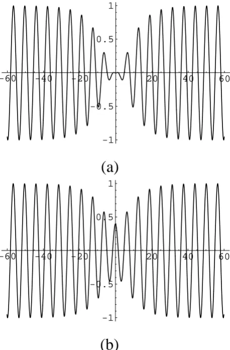
ForP Q < 0, the carrier wave is modulationally “stable” and may propagate as a “dark” (“black” or “grey”) envelope wavepackets, i.e. a propagating localized “hole” (a “void”) amidst a uniform wave energy region. The exact expres-sion for “dark” envelopes reads (Fedele and Schamel, 2002a; Fedele et al., 2002b)8:

ψ0=ψ00

tanh

_X−v

eT

L0

,

2= 1 2P

veX+ 2P Qψ00 2

−v

2

e 2

T (18)

(see Fig. 7a); again,L0ψ0₀=(2|P /Q|)1/2(=cst.).

8_{These expressions are readily obtained from (Fedele and}

Schamel, 2002a; Fedele et al., 2002b), by shifting the variables therein to our notation as:x→X, s→T, ρm→ρ0, α→2P,

q0→ −2P Q, 1→L, E→, V0→u.

-5 5 10 15 20 25

-1 -0.75 -0.5 -0.25 0.25 0.5 0.75 1

(a)

-5 5 10 15 20 25

-1 -0.75 -0.5 -0.25 0.25 0.5 0.75 1

(b)

-5 5 10 15 20 25

-1 -0.75 -0.5 -0.25 0.25 0.5 0.75 1

(c)

-5 5 10 15 20 25

-1 -0.75 -0.5 -0.25 0.25 0.5 0.75 1

(d)

-5 5 10 15 20 25

-1 -0.75 -0.5 -0.25 0.25 0.5 0.75 1

(e)

Fig. 5. Bright envelope soliton propagation, at different timest1 <· · ·< t5(arbitrary parameter values): cf. the structures encountered in satellite observations, e.g. see Fig. ??.

33

Fig. 5. Bright envelope soliton propagation, at different timest1<

· · ·< t5(arbitrary parameter values): cf. the structures encountered

-1 -0.5 0.5 1

-1 -0.75 -0.5 -0.25 0.25 0.5 0.75 1

(a)

-1 -0.5 0.5 1

-1 -0.75 -0.5 -0.25 0.25 0.5 0.75 1

(b)

-1 -0.5 0.5 1

-1 -0.75 -0.5 -0.25 0.25 0.5 0.75 1

(c)

-1 -0.5 0.5 1

-1 -0.75 -0.5 -0.25 0.25 0.5 0.75 1

(d)

-1 -0.5 0.5 1

-1 -0.75 -0.5 -0.25 0.25 0.5 0.75 1

(e)

Fig. 6. Bright envelope soliton profile (centered), at different timest1<· · ·< t5(arbitrary parameter values). Contrary to the previous figure, the envelope width here is comparable in order of magnitude to the carrier wavelength. Notice the variation in the localized packet’s internal structure, due to the (slow) phase variation in time.

34

Fig. 6. Bright envelope soliton profile (centered), at different times t1<· · ·< t5(arbitrary parameter values). Contrary to the previous

figure, the envelope width here is comparable in order of magni-tude to the carrier wavelength. Notice the variation in the localized packet’s internal structure, due to the (slow) phase variation in time.

-60 -40 -20 20 40 60

-1 -0.5 0.5 1

(a)

-60 -40 -20 20 40 60

-1 -0.5 0.5 1

(b)

Fig. 7. Dark-type modulated wavepackets (for

P Q <

0

) of the black (left) and grey (right) kind. See that the

amplitude never reaches zero in the latter case.

35

Fig. 7. “Dark”-type modulated wavepackets (forP Q < 0) of (a) “black” and (b) “grey” kind. See that the amplitude never reaches zero in the latter case.

5.3 Grey-type envelope solitons

The “grey”-type envelope (also obtained for P Q < 0) is given by (Fedele and Schamel, 2002a; Fedele et al., 2002b)8_:

ψ0 = ψ000

1−d2sech2

_X−v

eT

L00

1/2

and

2= 1 2P

V0X −

₁

2V

2

0 −2P Qψ

002 0

T +20

−S sin−1 d tanh X−veT

L00

1−d2_sech2

X−veT L00

1/2. (19)

Here 20 is a constant phase; S denotes the product

S = sign(P ) ×sign(ve −V0). The pulse width L00 =

(|P /Q|)1/2/(dψ000)now also depends on the real parameter d, given by:

d2 = 1 + (ve−V0)2/(2P Qψ00

(a)

(b)

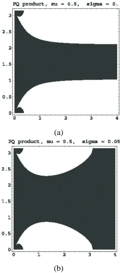
Fig. 8. The region of positive (negative) values of the product

P Q

, i.e. related to modulational instability

(stability), are depicted in white (black), in the wavenumber

k

(horizontal axis) - modulation angle

α

(vertical

axis) plane. These plots refer to ion-acoustic waves: (a)

σ

= 0

(cold model); (b)

σ

= 0

.

05

(warm model)

[Reprinted from (Kourakis and Shukla, 2004b)].

36

Fig. 8. The region of positive (negative) values of the productP Q, i.e. related to modulational instability (stability), are depicted in white (black), in the “wavenumber”k(horizontal axis) – “modula-tion angle”α(vertical axis) plane. These plots refer to “ion-acoustic waves”: (a)σ = 0 (cold model); (b) σ = 0.05 (warm model) (reprinted from Kourakis and Shukla, 2004b).

The (real) velocity parameterV0 = const.satisfies (Fedele

and Schamel, 2002a; Fedele et al., 2002b)8:

V0−

q

2|P Q|ψ002

0 ≤ ve ≤ V0+

q

2|P Q|ψ002 0.

Ford =1 (thusV0 =ve), one recovers the “dark” envelope soliton.

(a)

(b)

Fig. 9. Similar to Fig. ??, but for dust-ion acoustic waves (see in the text): (a)

σ

= 0

(cold model); (b)

σ

= 0

.

05

(warm model). We have considered a negative dust charge:

δ

=

qd,

/qi,

= 0

.

5

[i.e.

µ

=

ne,

/

(

Zini,

) =

0

.

5

]. The dust presence strongly modifies the stability profile, enhancing instability here [Reprinted from

(Kourakis and Shukla, 2004b)].

37

Fig. 9. Similar to Fig. 8, but for “dust-ion acoustic waves” (see in the text): (a)σ =0 (cold model); (b)σ =0.05 (warm model). We have considered a “negative” dust charge:δ=qd,0/qi,0=0.5 (i.e.

µ=ne,0/(Zini,0)=0.5). The dust presence strongly modifies the

stability profile, enhancing instability here (reprinted from Kourakis and Shukla, 2004b).

6 Explicit examples – known plasma modes

0 1 2 3 4 0

0.5 1 1.5 2 2.5 3

PQ product , mu = 1.5, sigma = 0.

(a)

0 1 2 3 4

0 0.5 1 1.5 2 2.5 3

PQ product , mu = 1.5, sigma = 0.05

(b)

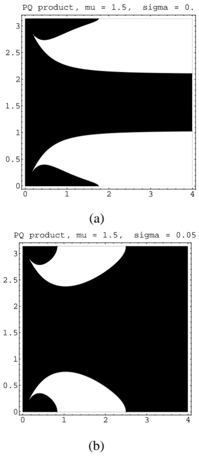
Fig. 10. Similar to Fig. ??, but for dust-ion acoustic waves in the presence of a positive dust charge: (a)

σ

= 0

(cold model); (b)

σ

= 0

.

05

(warm model). We have taken

δ

=

qd,

/qi,

= 0

.

5

[i.e.

µ

=

ne,

/

(

Zini,

) = 1

.

5

].

The positive dust charge seems to favor stability (cf. to the previous figure) [Reprinted from (Kourakis and

Shukla, 2004b)].

38

Fig. 10. Similar to Fig. 8, but for dust-ion acoustic waves in the presence of a “positive” dust charge: (a)σ = 0 (cold model); (b) σ =0.05 (warm model). We have takenδ=qd,0/qi,0=0.5 (i.e.

µ=ne,0/(Zini,0)=1.5). The positive dust charge seems to favor

stability (cf. to the previous figure) (reprinted from Kourakis and Shukla, 2004b).

6.1 Ion-acoustic waves

The main result of previous studies of the parallel modula-tion of ion-acoustic waves, namely the existence of a critical wavenumber, saykcr, above which the productP Qbecomes positive (i.e. instability may set in), is reproduced via the for-malism presented here.

6.1.1 Obliquity effects

Allowing for obliquity (by an angleθ) between the modula-tion and propagamodula-tion direcmodula-tions (cf. the early study by Kako and Hasegawa, 1976) was shown to modify the wave’s sta-bility profile rather dramatically: the value ofkcr reduces for small values ofθ (say, up to 0.4 rad, roughly) and then increases to infinity (prescribing stability) for higherθ; IA waves are globally stable to trasverse modulation (forθ =

π/2): observe the black region in Fig. 8a. 6.1.2 Thermal effects

Furthermore, allowing for a finite ion temperature (“warm” model, i.e.σ 6= 0; see Eqs. (4)–(6) above), one witnesses a dramatic modification of the stability profile, mainly via the appearance of a second wavenumber threshold, beyond which stability is recovered: short carrier wavelengths are stable in this “warm” description (cf. Figs. 8a and 8b), as first suggested by Chhabra and Sharma (1986).

6.2 Dust effects

The oblique modulation of the “dust-ion acoustic” and dust-acoustic ES plasma modes (Shukla and Mamun, 2002) was studied in (Amin et al., 1998; Kourakis and Shukla, 2003a, 2004b) and (Tang and Xue, 2003; Kourakis and Shukla, 2004a), respectively. The generic profile outlined above was here also recovered.

The presence of negative dust particulates was shown to modify the IA wave stability profile, by slightly favoring in-stability. In the case of positive dust, on the other side, stabil-ity was slightly enhanced instead. These results are depicted in Figs. 9 and 10 (to be compared to Fig. 8). A similar qual-itative behaviour was witnessed for the DA mode (Tang and Xue, 2003; Kourakis and Shukla, 2004a).

6.3 Two-temperature effects

The co-existence of distinct electron populations, say “hot” and “cold” electrons, which is observed in the boundaries of the Earth’s magnetosphere, has been shown to affect the modulation behaviour of ion acoustic (Kourakis and Shukla, 2003b) and electron-acoustic waves (Kourakis and Shukla, 2004d). Some of those results are depicted in Figs. 11 to 12, where the presence of the minority electrons appears to yield an important effect even in regions which would have been stable otherwise. Notice the appearance of new instability regions, even for high values of the modulation angle (lateral modulation).

7 Discussion and conclusion

0 0.5 1 1.5 2 0

0.5 1 1.5 2 2.5 3

PQ product, nu = 1004, mu=10

(a)

0 0.5 1 1.5 2

0 0.5 1 1.5 2 2.5 3

PQ product, nu = 1005, mu=10

(b)

Fig. 11. Similar to Fig. ??a (

σ

= 0

, i.e. cold model), but for ion acoustic waves in the presence of two

background electron populations (hot and cold electrons; the former are dominant here). Parameter values are:

(a) density ratio

ν

=

nh/nc

= 100

/

4 = 25

/

1

, temperature ratio

µ

=

Th/Tc

= 10

; (b)

ν

=

nh/nc

=

100

/

5 = 20

/

1

, temperature ratio

µ

=

Th/Tc

= 10

[reprinted from (Kourakis and Shukla, 2003b)].

39

Fig. 11. Similar to Fig. 8a (σ = 0, i.e. cold model), but for ion acoustic waves in the presence of two background electron popu-lations (“hot” and “cold” electrons; the former are dominant here). Parameter values are: (a) density ratioν = nh/nc = 100/4 = 25/1, temperature ratioµ = Th/Tc = 10; (b) ν = nh/nc = 100/5=20/1, temperature ratioµ=T_h/Tc=10 (reprinted from Kourakis and Shukla, 2003b).

amplitude in space and time may be modeled via the long-established multiple scale (“reductive perturbation”) method (Taniuti and Yajima, 1969; Asano et al., 1969). One thus ob-tains explicit conditions for the occurrence of “modulational instability”, which is related to wave collapse, or may possi-bly result in the formation of “localized envelope structures”. The criteria thus obtained, in terms of the systems’s physi-cal parameters, determine the wave’s modulational stability profile and predict the occurrence of localized envelope

ex-0 0.5 1 1.5 2 2.5 3

0 0.5 1 1.5 2

2.5 3

P Q product, beta = 0.5

modulation angle (rad)

wavenumber k / k

θ

(a)

0 0.5 1 1.5 2 2.5 3

0 0.5 1 1.5 2

2.5 3

P Q product, beta = 5

modulation angle (rad)

wavenumber k / k

θ

(b)

Fig. 12. A

{

k

−

θ

}

-plane plot qualitatively similar to Fig. ??a (for

σ

= 0

, i.e. cold model), but for electron

acoustic waves in the presence of two background electron populations. Parameter values are: (a) density ratio

ν

=

n

/n

= 2

/

1

(hot electrons dominant); (b)

ν

=

n

/n

= 1

/

5

(cold electrons dominant) [reprinted from

(Kourakis and Shukla, 2004d)].

40

Fig. 12. A{k−θ}-plane plot qualitatively similar to Fig. 8a (for σ = 0, i.e. cold model), but for “electron acoustic waves” in the presence of two background electron populations. Parameter values are: (a) density ratioν = nh/nc =2/1 (hot electrons dominant); (b)ν = nh/nc = 1/5 (cold electrons dominant) (reprinted from Kourakis and Shukla, 2004d).

where the electrostatic mode considered may be subject to Landau (collisionless) damping. As a matter of fact, this is not an issue in the case of dusty plasma modes (IAW, DAW), where the wave’s phase speed lies far from the characteristic thermal velocities of the constituents (Verheest, 2001; Shukla and Mamun, 2002). However, this should be taken into ac-count in the analysis, e.g. with respect to electron-acoustic waves (see the discussion in Kourakis and Shukla, 2004d), since it is known that Landau damping effects (obtained via a kinetic description of ES modes) cannot be predicted by fluid models.

The methodology employed in this article applies in a vari-ety of known electrostatic modes, which can be described by a single fluid model. A generalization of this formalism for plasma modes in the presence of an external magnetic field is on the way and will be reported soon.

Appendix A Perturbative analysis – details

A1 Harmonic amplitude evolution equations

By substituting into Eqs. (4)–(6) and (10) and isolating dis-tinct orders in, we obtain thenth-order reduced equations

−ilωn(n)_l + ilk·u(n)_l −λ∂n

(n−1) l

∂X

+∂n (n−2) l

∂T +

∂u(n_l,x−1) ∂X

+ ∞

X

n0₌₁

∞

X

l0_=−∞

ilk·u(n−n

0

) l−l0 n

(n0) l0 + ∂ ∂X n(n 0 ) l0 u

(n−n0−1) (l−l0_),x

= 0, (A1)

−ilωu(n)_l + s ilkφ_l(n) − λ∂u

(n−1) l

∂X +

∂u(n_l −2)

∂T

+s∂φ

(n−1) l

∂X xˆ

+ ∞

X

n0₌₁

∞

X

l0_=−∞

il0k·u(n−n

0

) l−l0 u

(n0) l0 + u

(n−n0−1) (l−l0_),x

∂u(n_l00)

∂X

+σ

ilp(n)_l k + ∂p (n−1) l

∂X xˆ

+ ∞

X

n0₌₁

∞

X

l0_=−∞

n(n−n

0

) (l−l0₎

−il0ωu(n

0

) l0 + s il

0 kφ(n

0

) l0

−λ∂u

(n0₋₁₎

l0

∂X +

∂u(n_l00−2)

∂T +s

∂φ_l(n0 0−1)

∂X xˆ

+ ∞

X

n00₌₁

∞

X

l00_=−∞

il00k·u(n_l0₋0−_l00n00)u

(n00₎

l00

+u(n_(l00₋−_ln0000_),x−1)

∂u(n_l0000)

∂X

= 0, (A2)

−ilωp(n)_l +ilγk·u(n)_l − λ∂p

(n−1) l

∂X

+∂p (n−2) l

∂T +γ

∂u(n_l,x−1) ∂X

+γ

∞

X

n0₌₁

∞

X

l0_=−∞

p(n−n

0

) l−l0

il0k·u(n

0

) l0 +

∂u(n

0₋

1) l0_,x

∂X

+ ∞

X

n0₌₁

∞

X

l0_=−∞

il0k·u(n_l−−_l0n0)p

(n0₎

l0 +

∂u(n

0₋

1) l0

∂X u

(n−n0₎

(l−l0_),x

= 0, (A3)

and

−(l2k2+1) φ_l(n) +s β n(n)_l

+2ilkx

∂φ_l(n−1)

∂X +

∂2φ(n_l −2) ∂X2

+α

∞

X

n0₌₁

∞

X

l0_=−∞

φ(n−n

0

) l−l0 φ

(n0) l0

−α0

∞

X

n0_,n00₌₁

∞

X

l0_,l00_=−∞

φ_l(n₋−_l0₋n0_l−00n00)φ

(n0₎

l0 φ

(n00₎

l00

= 0. (A4)

A2 First order in: first harmonics and dispersion relation The first order (n=2) equations read

−ilωn(_l1) +ilk·u(_l1) = 0, (A5) −ilωu(_l1) + s ilkφ_l(1) +ilσ p(_l1)k = 0, (A6) −ilωp_l(1) +ilγk·u(_l1) = 0, (A7) and

−(l2k2+1) φ_l(1) +s β n(_l1) = 0. (A8) Forl =1, these equations determine the first harmonics of the perturbation. The following dispersion relation is ob-tained

ω2 = β k

2

k2₊₁ +γ σ k

2_{. (A9)}

Restoring dimensions, one may easily check that the stan-dard DAW dispersion relation (Rao et al., 1990; Shukla and Mamun, 2002) is thus exactly recovered:

ω2 =ω2_p,d k 2 k2_+k2

D

+γ kBTd md

k2

= ≡ c

2

Dk2 1+k2_λ

D2_eff

+ γ v_{t h,d}2 k2. (A10)

the relations

n(₁1) =s1+k 2 β φ

(1)

1

≡c₁(11)φ₁(1),

k·u(₁1) = ω n₁(1) =s ω1+k 2

β φ

(1)

1

≡c₂(11)φ₁(1),

p(₁1) =γ n(₁1) =γ s1+k 2 β φ

(1)

1

≡c₃(11)φ₁(1),

u(₁1_,x) =ω

k cosθ n

(1)

1 =s

1+k2 β

ω k cosθ φ

(1)

1

≡c₅(11)φ₁(1),

u(₁1_,y) =ω

k sinθ n

(1)

1 =s

1+k2 β

ω k sinθ φ

(1)

1 , (A11)

retaining, for later use, the (obvious) definitions of the coef-ficientsc(_j11)(j =1, ...,5) relating the state variables to the 1st-order potential correctionφ₁(1)(soc₄(11)=1).

A3 Second order in: group velocity, 0th and 2nd harmon-ics

The second order (n = 2) equations for the first harmonics provide the compatibility condition: λ = vg(k) = _∂k∂ω_x =

ω0(k)cosθ = k ω

1

(1+k2₎2 +γ σ

cosθ; the group velocityvg can be cast in the form

vg(k)=

ω3 k3

β+σ γ (1+k2)2

[β+σ γ (1+k2_)]2cosθ≡ ω3

βk3ν1cosθ, (A12)

where we have denoted

ν1=β β+σ γ (1+k 2₎2

[β+σ γ (1+k2_)]2. (A13)

Note thatν1 → 1 in the limitσ → 0, recovering exactly

Eq. (43) in (Amin et al., 1998).

The 2nd-order corrections to the first harmonic amplitudes are now given by

n(₁2) =i s 1 β

_˜

A(1+k2)−2kcosθ∂φ

(1)

1 ∂X

≡i c(₁21)∂φ

(1)

1 ∂X ,

k·u(₁2) =ωn(₁2)−s1 β (1+k

2₎

vg−

ω k cosθ

_∂φ(1)

1 ∂X

≡i c(₂21)∂φ

(1)

1 ∂X , p(₁2) =γ n(₁2)

≡ i c(₃21)∂φ

(1)

1 ∂X ,

φ₁(2)=iA˜∂φ

(1)

1 ∂X ,

and

u(₁2_,x) =i s1 ω

−1−2γ

β σ k 2 _cos2_θ

+

vg

ω

k cosθ−σ γ

₁₊

k2 β

_∂φ(1)

1 ∂X ,

≡ i c₅(21) ∂φ

(1)

1

∂X . (A14)

The choice of the value ofA˜is arbitrary; we shall takeA˜=0. The equations forn=2,l=2 provide the amplitudes of the second order harmonics, which are found to be propor-tional to the square of the correspondingS₁(1) elements e.g. in terms ofφ₁(1)

n(₂2) =

₁

ωA +

(1+k2)2 β2

≡ c(₁22)φ₁(1)2,

k·u(₂2) = (1+k

2_{) ω}

6β3_k2

2s α β2 +3β (1+k2)(1+2k2)

+2γ2σ (1+k2)2(1+4k2)

φ(₁1)2

≡ A φ₁(1)2 =c₂(22)φ(₁1)2,

p(₂2) = γ

₁

ωA+γ

(1+k2)2 β2

≡ c₃(22)φ₁(1)2,

and

φ(₂2) = 1 4k2₊₁

s β

₁

ωA +

(1+k2)2 β2

+ α

φ₁(1)2

≡ c(₄22)φ₁(1)2. (A15)

Notice that these expressions are “isotropic” i.e. independent of the value ofθ.

The nonlinear self-interaction of the carrier wave also re-sults in the creation of a zeroth harmonic, in this order; its strength is analytically determined by taking into account the

l =0 component of the three first third-order reduced equa-tions (i.e. Eqs. (A1)–(A3) forn = 3, l = 0) together with the corresponding fourth 2nd-order equation (i.e. Eq. (A4) forn =2, l = 0). The result is conveniently expressed in terms of the square modulus of the (n=1,l=1) quantities, e.g. in terms of|φ(₁1)|2=(φ₁(1))∗φ₁(1)

n(₀2) = −1

β+γ σ−v2

g 1

β

1+2sαβ +k2 +2 cos2θ

+γ σ (1+k 2₎2

β (γ +2 cos

2_θ−1)|φ(1)

1 | 2

≡ B|φ₁(1)|2 ≡ = c₁(20)|φ(₁1)|2,

k·u(₀2) = −1

β+γ σ−v2

g cosθ

β2

2ω (β+γ σ )(1+k2)2

×cosθ

+k vg

+σ γ (γ −1)(1+k2)2

≡ c(₂20)|φ₁(1)|2, p(₀2) = γ

B + 1

β2(γ −1) (1+k 2₎2₎

|φ₁(1)|2

≡ c(₃20)|φ₁(1)|2, φ₀(2) = (s β B +2α)|φ₁(1)|2

≡ c(₄20)|φ₁(1)|2, (A16) and

u(₀2_,x) =

vgB −2

ω (1+k2)2 β2_k cosθ

|φ₁(1)|2

≡ c₅(20)|φ(₁1)|2. (A17) It is expected, and indeed verified by a tedious yet straightfor-ward calculation, that upon settingσ =0,s= −1 in expres-sions (A15) and (A16), one recovers exactly Eqs. (44)–(49) in (Amin et al., 1998) (given Eq. (42) therein).

Notice, for rigor, that for “vanishing obliqueness” i.e. if

θ→0, one obviously has k·u(n)_l →k u(n)_l (by definition), implying the condition:c(nl)₂ →k c(nl)₅ (forθ→0) which is indeed satisfied for alln,l, by the above formulae.

A4 Derivation of the Nonlinear Schr¨odinger Equation Proceeding to the third order in (n = 3), the equation for l = 1 yields an explicit compatibility condition to be imposed on the right-hand side of the evolution equations which, given the expressions derived previously, can be cast into the form

A1 dψ dT +i A2

d2ψ

dX2 +i A3|ψ|

2_{ψ=0, (A18)}

where ψ ≡ φ(₁1) denotes the amplitude of the first-order electric potential perturbation; coefficients A1,2,3 are to be

defined. Now, multiplying byi A−₁1, we obtain the familiar form of the Nonlinear Schr¨odinger Equation

i∂ψ ∂T +P

∂2ψ

∂X2 +Q|ψ|

2_{ψ=0. (A19)}

Recall that the “slow” variables {X, T} were defined in Sect. 2.

The “dispersion coefficient” P = −A2/A1 is related to the curvature of the dispersion curve as

P = 1 2

∂2ω ∂k2

x = 1

2

ω00(k)cos2θ +ω0(k)sin 2_θ k

;

the exact form of P reads

P (k) = 1

β

1 2ω

_ω

k

4

ν1−(ν1+3 ν2

β ω

2_)cos2_θ,(A20)

where we have defined

ν2=β33β+γ σ (3−k

2_)(1+k2₎

3[β+γ σ (1+k2_)]4 . (A21)

Note that, just likeν1defined above,ν2 →1 whenσ → 0; see that relation (51) in (Amin et al., 1998) is recovered from Eq. (A20) in this case. If, furthermore, we setβ =1 (in ad-dition toσ =0) in all expressions describing our dispersion law i.e. Eqs. (A9), (A12), (A20) above, we obtain, respec-tively, Eqs. (3), (11), (4) in (Kako and Hasegawa, 1976).

It seems appropriate, here, to point out the qualitative dif-ference betweenP given in Eq. (A20) as compared to rele-vant previous expressions: the existence ofσ may affect the sign of theP coefficient. For instance, takingσ = 0 (i.e.

ν1 = ν2 = 1),P is readily seen to be negative for parallel

modulation, i.e. settingθ=0; however, forσ 6=0 this is no longer the case, sinceP changes sign at some critical value ofk(to see this, study the sign ofν2versusk). Furthermore, a similar remark holds for the effect of an oblique modula-tion on the sign ofP; we will come back to this subtle point in the next subsection.

The “nonlinearity coefficient”Q= −A3/A1is due to the carrier wave self-interaction. Distinguishing different contri-butions,Qcan be split into five distinct parts, viz.

Q= Q0 +Q1 + Q2 +Q3 + Q4, (A22)

reflecting the similar structure ofA3 A3= A(30) + A

(1)

3 + A

(2)

3 + A

(3)

3 +A

(4)

3 . (A23)

In order to trace the influence of the various parameters, let us define all quantities in full detail. First,A(₃0) (as well as

Q0= −A(30)/A1) is related to the self-interaction due to the

zeroth harmonic, viz.

A₃(0)= −β k2(c(₁11)c₂(20) +c(₂11)c₁(20))

−s ω2α k2c(₄11)c₄(20) − ω (1+k2) c₂(11)c(₂20),

(A24) whileA(₃2)(related toQ2= −A(₃2)/A1) is the analogue quan-tity due to the second harmonic

A₃(2)= −β k2(c(₁11)c₂(22) +c(₂11)c₁(22))

−s ω2α k2c(₄11)c₄(22) − ω (1+k2) c₂(11)c(₂22).

(A25) All coefficientsc_j(nl) were defined previously. Now, Q1 = −A(₃1)/A1 is simply the nonlinearity contribution from the cubic term in Eq. (10d) (often omitted in the past)

A₃(1)= +3s α0ω (c₄(11))3k2, (A26) Finally,A(₃3) (related toQ3= −A(₃3)/A1) is the (σ-related)

result of the third line in Eq. (A2)

A(₃3)= −σ k2(1+k2)

γ c₂(11)(c₃(20)− c₃(22))

+2γ c(₃11)c₂(22)+c(₃11)(c(₂20)

−c₂(22)) +2c(₂11)c(₃22)

whileA(₃4)(andQ4= −A(₃4)/A1) is due to the last two lines in Eq. (A2)

A(₃4)= −ω (1+k2)

(ω c(₂11)−sk2c₄(11)) (c(₁22)−c(₁20))

−2c(₁11)(ω c₂(22)−sk2c₄(22)) + (c(₂11))2c₁(11)

. (A28) We note thatA1is everywhere defined as

A1= −s 2 β (1+k

2₎2_ω2_{, (A29)}

i.e. by using Eq. (A9)

A−₁1= −s 1

2β

1

ω2

_ω2 k2 −γ σ

2

(A30) (reducing to:A−₁1= −s₂1_β ω2

k4 forσ =0). Remember that

Q3 andQ4 are plainly absent from the previous results in

(Amin et al., 1998) – i.e. forσ =0 – and so is, in fact,Q1.

Substituting from the expressions derived above for the co-efficientsc(nl)_j and re-arranging, we obtain

Q0= + 1 2ω

1

β2

1

(1+k2₎2

1

β+γ σ−v2

g ×

β k2

β3+6k2+4k4+k6

+2α β s (2k2+3)+2α v_g2

+γ σ(γ +1) (1+k2)3

+2α β −2αβ+s γ (1+k2)2

+β (2+4k2+3k4+k6+2sαβ)

+2γ σ (1+k2)2(1+k2+sαβ)cos 2θ

+2(1+k2)4(β+γ σ ) ω2 cos2θ

+k (1+k2)

βk2+ω2(1+k2)

_v

g

ω ×

β (1+k2+2sαβ) +γ (γ −1) σ (1+k2)2

×cosθ

, (A31)

Q1=

3α0β

2ω k2

(1+k2₎2, (A32)

Q2= −

1 12β3

1

ω

1

k2_(1+k2₎2 ×

2β k2

5s α β2(1+k2)2+ 2α2β3

+2γ2σ (1+k2)4(1+4k2)

+β (1+k2)3(3+9k2+2s α γ2σ )

+(1+k2)3ω2

β (3+9k2+6k4+2sαβ)

+2γ2σ (1+k2)2(1+4k2)

. (A33)

Finally, the coefficients Q3 = −A(₃3)/A1 and Q4 = −A(₃4)/A1can be directly computed from Eq. (A27)–(A29) above; the lengthy final expressions are omitted here.

Once substituted in Eq. (A22), these expressions provide the final expression for the nonlinearity coefficientQ. One may readily check, yet after a tedious calculation, that ex-pressions (A31) and (A33) reduce to Eqs. (53) and (54) in (Amin et al., 1998) forσ =0. However, the remaining coef-ficientsQ1,Q3,Q4were absent in all previous studies of the

DA waves, to the best of our knowledge. Their importance will be discussed in the following. Note thatQ1,Q2do not depend on the angleθ.

A5 Behaviour of coefficients for smallk

A preliminary result regarding the behaviour (and the sign) of the NLSE coefficientsP andQ, at least for long wave-lengths, may be obtained by considering the limit of small

k1 in the above formulae.

The parallel (θ=0) and oblique (θ6=0) modulation cases have to be distinguished straightaway. For small values ofk

(k1),P is negative and varies as

P

θ=0 ≈ −

3 2

β

√

β+γ σ k (A34)

in the parallel modulation case (i.e.θ =0), thus tending to zero for vanishingk, while forθ 6=0,P is positive and goes to infinity as

P

θ6=0 ≈

√

β+γ σ

2k sin

2_{θ (A35)}

for vanishingk. Therefore, the slightest deviation byθof the amplitude variation direction with respect to the wave prop-agation direction results in a change in sign of the dispersion coefficientP. Given the importance of the coefficient prod-uctP Q(to be discussed in the next Section), one may won-der whether this is sufficient for the stability characteristics of the DA wave to change. Let us see what happens with the

Qin the limit of smallk.

For all cases,Qvaries as∼1/ kfor smallk1; the exact expression in fact depends on the angleθ. In the general case (θ6=0), the result reads

Q_θ6=0 ≈ −

1 12β3

1 √

β+γ σ [β (2sαβ+3)+2γ 2_σ]

×[β (2sαβ+3)+γ (γ +1) σ]1

k. (A36)

A careful study shows thatQis negative, in fact, for all pos-sible values of the physical parameters of interest (i.e.α,β,

γ,σ – all positive – “and”s±1). For vanishing θ, how-ever, the approximate expression forQ, yet apparently quite similar, is now “positive”, i.e.

Q

θ=0 ≈ +

1 12β3

1 √

β+γ σ [β (2sαβ+3)+2γ σ]

×[β (2sαβ+3)+γ (γ +1) σ]1

Notice, for rigor, that these formulae are in agreement with the (known) case of the parallel-modulated ion-acoustic waves: see Eq. (41) in Shimizu and Ichikawa (1972); as a matter of fact, the factor 1/3 therein is also exactly recov-ered here upon setting the appropriate parameter values into Eq. (A37).

In conclusion, both coefficients P and Q change sign when switching on “theta”. Indeed, obliqueness in modu-lation is expected to influence the stability profile of the sys-tem; this point seems to confirm (and complete) the general qualitative arguments put forward in (Kako and Hasegawa, 1976) for the ion acoustic wave in an electron ion plasma without dust. Nevertheless, at all cases, the product ofP

andQis negative for smallk, ensuring, as we shall see in the following section, stability for long perturbation wave-lengths. As a by-product of this analysis, we see that taking into accountQ1,Q3andQ4does not seem to influence the dynamics in the low wavenumberkparameter range.

Acknowledgements. This work was supported by the SFB591

(Son-derforschungsbereich) – Universelles Verhalten gleichgewichts-ferner Plasmen: Heizung, Transport und Strukturbildung German government Programme, as well as the International Space Science Institute (ISSI), Bern, Switzerland.

I. Kourakis is grateful to Max-Planck-Institut f¨ur extraterrestrische Physik (Garching, Germany) for the award of a fellowship (project: “Komplexe Plasmen”).

Figure 1 is reprinted from: Santolik, O., Gurnett, D. A., Pickett, J. S., Parrot, M., and Cornilleau-Wehrlin, N.: Spatio-temporal struc-ture of storm-time chorus, J. Geophys. Res., 108, 1278/1-14 (2003); Copyright (2003) American Geophysical Union; reproduced by per-mission of the American Geophysical Union.

Figure 2 is reprinted from: Pottelette, R., Ergun, R. E., Treumann, R. A., Berthomier, M., Carlson, C. W., McFadden, J. P., and Roth, I.: Modulated electron-acoustic waves in auroral density cavities: FAST observations, Geophys. Res. Lett., 26, 16, 2629–2632, 1999; Copyright (1999) American Geophysical Union; reproduced by per-mission of the American Geophysical Union.

Figure 3 is reprinted from: Alpert, Ya.: Resonance nature of the magnetosphere, Physics Reports 339, 323–444, 2001; Copyright (2001) Elsevier; reproduced by permission of Elsevier.

Figures 8–10 is reprinted from: Kourakis, I. and Shukla, P. K.: Fi-nite ion temperature effects on the stability and envelope excitations of dust-ion acoustic waves, European Physical Journal D, 28, 109– 117, 2004; Copyright (2003) Springer; reproduced by permission of Springer.

Figure 11 is reprinted from: Kourakis, I. and Shukla, P. K.: Ion-acoustic waves in a two-electron-temperature plasma: oblique mod-ulation and envelope excitations, Journal of Physics A: Mathemati-cal & General, 36, 11 901–11 913, 2003; Copyright (2003) Institute of Physics.

Figure 12 is reprinted from: Kourakis, I. and Shukla, P. K.: Electron-acoustic plasma waves: oblique modulation and envelope solitons, Physical Review E, 69, 3, 036411/1-7, 2004; Copyright (2004) American Physical Society.

Edited by: J. F. McKenzie Reviewed by: two referees

References

Alpert, Ya.: Resonance nature of the magnetosphere, Physics Re-ports, 339, 323–444, 2001.

Amin, M. R., Morfill, G. E., and Shukla, P. K.: Modulational insta-bility of dust-acoustic and dust-ion-acoustic waves, Phys. Rev. E, 58, 6517–6523, 1998.

Asano, N., Taniuti, T., and Yajima, N.: Perturbation method for a nonlinear wave modulation II, J. Math. Phys., 10, 2020–2024, 1969.

Bailung, H., and Nakamura, Y.: Observation of modulational insta-bility in a multi-component plasma with negative ions, J. Plasma Phys., 50, 2, 231–242, 1993.

Berthomier, M., Pottelette, R., and Malingre, M.: Solitary waves and weak double layers in a two-electron temperature auroral plasma, J. Geophys. Res., 103, A3, 4261–4270, 1998.

Bostr¨om, R.: Characteristics of Solitary Waves and Weak Double Layers in the Magnetospheric Plasma, Phys. Rev. Lett., 61, 82– 85, 1988.

Cattell, C. A., Dombeck, J., Wygant, J. R., Hudson, M. K., Mozer, F. S., Temerin, M. A., Peterson, W. K., Kletzing, C. A., Russell, C. T., and Pfaff, R.: Comparisons of Polar satellite observations of solitary wave velocities in the plasma sheet boundary and the high altitude cusp to those in the auroral zone, Geophys. Res. Lett., 26, 425–428, 1999.

Cattell, C. A., Neiman, C., Dombeck, J., Crumley, J., Wygant, J., Kletzing, C. A., Peterson, W. K., Mozer, F. S., and Andr´e, M.: Large amplitude solitary waves in and near the Earth’s magneto-sphere, magnetopause and bow shock: Polar and Cluster obser-vations, Nonlin. Proc. Geophys., 10, 13–26, 2003,

SRef-ID: 1607-7946/npg/2003-10-13.

Chhabra, R. and Sharma, S.: Modulational instability of obliquely modulated ion-acoustic waves in a two-ion plasma, Phys. Fluids, 29, 128–132, 1986.

Chan, V. and Seshadri, S.: Modulational stability of the ion plasma mode, Phys. Fluids, 18, 1294–1298, 1975.

Davydov, A. S.: Solitons in Molecular Systems, Kluwer Academic Publishers, Dordrecht, 1985.

Delory, G. T., Ergun, R. E., Carlson, C. W., Muschietti, L., Chaston, C. C., Peria, W., and McFadden, J. P.: FAST observations of electron distributions within AKR source regions, Geophys. Res. Lett., 25, 12, 2069–2072, 1998.

Durrani, I. R., Murtaza, G., Rahman, H. U., and Azhar, I. A.: Ef-fect of ionic temperature on the modulational instability of ion acoustic waves in a collisionless plasma, Phys. Fluids, 22, 791– 793, 1979.

Eliasson, B. and Shukla, P. K.: Theoretical and numerical studies of density modulated whistlers, Geophys. Res. Lett., 31, L17802/1-4, 2004.

Ergun, R. E., Carlson, C. W., McFadden, J. P., Mozer, F. S., De-lory, G. T., Peria, W., Chaston, C. C., Temerin, M., Roth, I., Muschietti, L., Elphic, R., Strangeway, R., Pfaff, R., Cattell, C. A., Klumpar, D., Shelley, E., Peterson, W., Moebius, E., and Kistler, L.: FAST satellite observations of large-amplitude soli-tary structures, Geophys. Res. Lett., 25, 2041–2044, 1998a. Ergun, R. E., Carlson, C. W., McFadden, J. P., Mozer, F. S.,

Fedele, R. and Schamel, H.: Solitary waves in the Madelung’s Fluid: A Connection between the nonlinear Schr¨odinger equa-tion and the Korteweg-de Vries equaequa-tion, Eur. Phys. J. B, 27, 313–320, 2002a.

Fedele, R., Schamel, H., and P. K. Shukla: Solitons in the Madelung’s Fluid, Phys. Scripta, T98, 18–23, 2002b.

Franz, J. R., Kintner, P. M., and Pickett, J. S.: POLAR observations of coherent electric field structures, Geophys. Res. Lett., 25, 8, 1277–1280, 1998.

Hasegawa, A.: Stimulated Modulational Instabilities of Plasma Waves, Phys. Rev. A, 1, 6, 1746–1750, 1970.

Hasegawa, A.: Theory and Computer Experiment on Self-Trapping Instability of Plasma Cyclotron Waves, Phys. Fluids, 15, 5, 870– 881, 1972.

Hasegawa, A.: Plasma Instabilities and Nonlinear Effects, Springer-Verlag, Berlin, 1975.

Hasegawa, A.: Optical Solitons in Fibers, Springer-Verlag, 1989.