www.atmos-meas-tech.net/9/2119/2016/ doi:10.5194/amt-9-2119-2016
© Author(s) 2016. CC Attribution 3.0 License.
Algorithm update of the GOSAT/TANSO-FTS thermal infrared
CO
2
product (version 1) and validation of the UTLS CO
2
data
using CONTRAIL measurements
Naoko Saitoh1, Shuhei Kimoto1, Ryo Sugimura1, Ryoichi Imasu2, Shuji Kawakami3, Kei Shiomi3, Akihiko Kuze3, Toshinobu Machida4, Yousuke Sawa5, and Hidekazu Matsueda5
1Center for Environmental Remote Sensing, Chiba University, Chiba, Japan 2Atmosphere and Ocean Research Institute, University of Tokyo, Kashiwa, Japan 3Japan Aerospace Exploration Agency, Tsukuba, Japan
4National Institute for Environmental Studies, Tsukuba, Japan 5Meteorological Research Institute, Tsukuba, Japan
Correspondence to: Naoko Saitoh ([email protected])
Received: 15 October 2015 – Published in Atmos. Meas. Tech. Discuss.: 10 December 2015 Revised: 27 April 2016 – Accepted: 27 April 2016 – Published: 13 May 2016
Abstract. The Thermal and Near Infrared Sensor for Car-bon Observation (TANSO)–Fourier Transform Spectrome-ter (FTS) on board the Greenhouse Gases Observing Satel-lite (GOSAT) has been observing carbon dioxide (CO2)
con-centrations in several atmospheric layers in the thermal in-frared (TIR) band since its launch. This study compared TANSO-FTS TIR version 1 (V1) CO2data and CO2data
ob-tained in the Comprehensive Observation Network for TRace gases by AIrLiner (CONTRAIL) project in the upper tropo-sphere and lower stratotropo-sphere (UTLS), where the TIR band of TANSO-FTS is most sensitive to CO2concentrations, to
validate the quality of the TIR V1 UTLS CO2data from 287
to 162 hPa. We first evaluated the impact of considering TIR CO2averaging kernel functions on CO2concentrations using
CO2 profile data obtained by the CONTRAIL Continuous
CO2 Measuring Equipment (CME), and found that the
im-pact at around the CME level flight altitudes (∼11 km) was on average less than 0.5 ppm at low latitudes and less than 1 ppm at middle and high latitudes. From a comparison made during flights between Tokyo and Sydney, the averages of the TIR upper-atmospheric CO2data were within 0.1 % of the
averages of the CONTRAIL CME CO2data with and
with-out TIR CO2averaging kernels for all seasons in the
South-ern Hemisphere. The results of comparisons for all of the eight airline routes showed that the agreements of TIR and CME CO2data were worse in spring and summer than in fall
and winter in the Northern Hemisphere in the upper tropo-sphere. While the differences between TIR and CME CO2
data were on average within 1 ppm in fall and winter, TIR CO2 data had a negative bias up to 2.4 ppm against CME
CO2 data with TIR CO2 averaging kernels at the northern
low and middle latitudes in spring and summer. The nega-tive bias at the northern middle latitudes resulted in the max-imum of TIR CO2 concentrations being lower than that of
CME CO2concentrations, which led to an underestimate of
the amplitude of CO2seasonal variation.
1 Introduction
Carbon dioxide (CO2)in the atmosphere is a well-known
strong greenhouse gas (IPCC, 2013, and references therein), with concentrations that have been observed both in situ and by satellite sensors. Its long-term observation began in Mauna Loa, Hawaii, and the South Pole in the late 1950s (Keeling et al., 1976a, b, 1996). Since then, comprehensive CO2 observations in the atmosphere have been conducted
Atmo-spheric CO2 concentrations have gradually increased at a
globally averaged annual rate of 1.7±0.5 ppm from 1998 to 2011, although its growth rate has relatively large interan-nual variation (IPCC, 2013). Upper-atmospheric CO2
obser-vations have been made in many areas by several projects us-ing commercial airliners, such as the Comprehensive Obser-vation Network for TRace gases by AIrLiner (CONTRAIL) project (Machida et al., 2008) and the Civil Aircraft for the Regular Investigation of the atmosphere Based on an Instru-ment Container (CARIBIC) project (Brenninkmeijer et al., 2007). Continuous long-term measurements of CO2made by
several airplanes of Japan Airlines (JAL) in the CONTRAIL project have revealed details of its seasonal variation and in-terhemispheric transport in the upper atmosphere (Sawa et al., 2012) and interannual and long-term trends of its latitu-dinal gradients (Matsueda et al., 2015).
Atmospheric CO2 observations by satellite sensors are
categorized into two types: those utilizing CO2 absorption
bands in the shortwave infrared (SWIR) regions at around 1.6 and 2.0 µm, and those in the thermal infrared (TIR) re-gions at around 4.6, 10, and 15 µm. The Scanning Imag-ing Absorption Spectrometer for Atmospheric Chartogra-phy (SCIAMACHY) on the Environmental Satellite (EN-VISAT) first observed CO2 column-averaged dry-air mole
fractions (XCO2)from spectra at 1.57 µm (Buchwitz et al.,
2005; Barkley et al., 2006). The Thermal and Near Infrared Sensor for Carbon Observation (TANSO)–Fourier Transform Spectrometer (FTS) on board the Greenhouse Gases Ob-serving Satellite (GOSAT), which was launched in 2009 (Yokota et al., 2009), has observed XCO2with high
preci-sion by utilizing the 1.6 and/or 2.0 µm CO2absorption bands
(Yoshida et al., 2011, 2013; O’Dell et al., 2012; Butz et al., 2011; Cogan et al., 2012). The Orbiting Carbon Observatory 2 (OCO-2) was successfully launched in 2014 and started regular observations of XCO2 with high spatial resolution.
Satellite CO2observations at TIR absorption bands have a
longer history beginning with the High-Resolution Infrared Sounder (HIRS) (Chédin et al., 2002, 2003, 2005). The At-mospheric Infrared Sounder (AIRS) has achieved more ac-curate observations of middle- and upper-tropospheric CO2
concentrations (Crevoisier et al., 2004; Chahine et al., 2005; Maddy et al., 2008; Strow and Hannon, 2008). The Tro-pospheric Emission Spectrometer (TES) has observed CO2
concentrations in several vertical layers with high accuracy by taking advantage of its high wavelength resolution (Ku-lawik et al., 2010, 2013). The Infrared Atmospheric Sound-ing Interferometer (IASI) has observed upper-atmospheric CO2amounts from its TIR spectra (Crevoisier et al., 2009).
TANSO-FTS also has a TIR band in addition to its three SWIR bands, and it obtains vertical information of CO2
con-centrations in addition to XCO2 in the same field of view
(Saitoh et al., 2009).
Rayner and O’Brien (2001) and Pak and Prather (2001) showed the utility of global CO2 data obtained by
satel-lite sensors for estimating its source and sink strength, and
many studies of CO2inversion have been conducted using a
huge amount of satellite data since the 2000s. Chevallier et al. (2005) first used satellite CO2data, observed with the
Op-erational Vertical Sounder (TOVS), to estimate CO2surface
fluxes. They reported that a regional bias in satellite CO2data
hampers the outcomes. Nassar et al. (2011) demonstrated that the wide spatial coverage of satellite CO2data is
ben-eficial to CO2 surface flux inversion through the combined
use of TES and surface flask CO2 data, particularly in
re-gions where surface measurements are sparse. In addition to CO2surface inversion results using TIR observations, global
XCO2data observed with the SWIR bands of TANSO-FTS
have been actively used for estimating CO2source and sink
strength (Maksyutov et al., 2013; Saeki et al., 2013a; Cheval-lier et al., 2014; Basu et al., 2013, 2014; Takagi et al., 2014). One of the important things to consider when incorporating satellite data in CO2 inversion is the accuracy of the data,
as suggested by Basu et al. (2013). Uncertainties in satel-lite CO2data should be assessed seasonally and regionally
to determine the seasonal and regional characteristics of the satellite CO2bias.
The importance of upper-atmospheric CO2 data in the
inversion analysis of CO2 surface fluxes was discussed
in Niwa et al. (2012). They used CONTRAIL CO2 data
in conjunction with surface CO2 data to estimate surface
flux, and they demonstrated that adding middle- and upper-tropospheric data observed by the aircraft could greatly reduce the posteriori flux errors, particularly in tropical Asian regions. Middle- and upper-tropospheric and lower-stratospheric CO2 concentrations and column amounts of
CO2 can be simultaneously observed in the same field of
view with TANSO-FTS on board GOSAT. Provided that the quality of upper-atmospheric CO2 data simultaneously
ob-tained with TANSO-FTS is proven to be comparable to that of TANSO-FTS XCO2 data (Yoshida et al., 2013; Inoue et
al., 2013), the combined use of upper-atmospheric CO2and
XCO2 data observed with TANSO-FTS could be a useful
tool for estimating CO2surface flux.
GOSAT, which is the first satellite to be dedicated to green-house gas monitoring, was launched on 23 January 2009. As described above, TANSO-FTS on board GOSAT has been observing CO2concentrations in several vertical layers in the
TIR band. In this study, we focused on CO2concentrations
in the upper troposphere and lower stratosphere (UTLS), where the TIR band of TANSO-FTS is most sensitive. We validated these data by comparison with upper-atmospheric CO2 data obtained in a wide spatial coverage in the
CON-TRAIL project. Sections 2 and 3 explain the GOSAT and CONTRAIL measurements, respectively. Section 4 details the retrieval algorithm used in the latest version 1 (V1) CO2
level 2 (L2) product of the TIR band of TANSO-FTS. Sec-tion 5 describes the methods of comparing TANSO-FTS TIR V1 L2 and CONTRAIL CO2data. Sections 6 and 7 show
2 GOSAT observations
GOSAT is a joint satellite project of the National Insti-tute for Environmental Studies (NIES), Ministry of the Environment (MOE), and Japan Aerospace Exploration Agency (JAXA) for the purpose of making global observa-tions of greenhouse gases such as CO2and CH4(Hamazaki
et al., 2005; Yokota et al., 2009). It was launched on 23 January 2009, from the Tanegashima Space Center, and has continued its observations for more than 6 years. GOSAT is equipped with TANSO-FTS for greenhouse gas monitor-ing and the TANSO-Cloud and Aerosol Imager (CAI) to de-tect clouds and aerosols in the TANSO-FTS field of view (Kuze et al., 2009). TANSO-FTS consists of three bands in the SWIR region and one band in the TIR region. Col-umn amounts of greenhouse gases are observed in the SWIR bands, and vertical information of gas concentrations are ob-tained in the TIR band (Yoshida et al., 2011, 2013; Saitoh et al., 2009, 2012; Ohyama et al., 2012, 2013).
Kuze et al. (2012) provided a detailed description of the methods used for the processing and calibration of level 1B (L1B) spectral data from TANSO-FTS. They explained the algorithm for the version 150.151 (V150.151) L1B spec-tral data. The TIR V1 L2 CO2 product we focused on in
this study was created from a later version, V161.160, of L1B spectral data. The following modifications were made to the algorithm from V150.151 to V161.160: improving the TIR radiometric calibration through the improvement of calibration parameters, turning off the sampling interval non-uniformity correction, modifying the spike noise crite-ria of the quality flag, and reevaluating the misalignment be-tween the GOSAT satellite and TANSO-FTS sensor. Kataoka et al. (2014) reported that the biases of TANSO-FTS TIR V130.130 L1B radiance spectra based on comparisons with the Scanning High-resolution Interferometer Sounder (S-HIS) spectra for warm scenes were 0.5 K at 800–900 and 700–750 cm−1, 0.1 K at 980–1080 cm−1, and more than 2 K at 650–700 cm−1. Although the magnitude of the spectral bias evaluated on the basis of V130.130 L1B data would change in V161.160 L1B data, the issue of L1B spectral bias still remains. The spectral bias inherent in TIR L1B spec-tra would be mainly because of uncertainty of polarization correction. Another possible cause was discussed in Imasu et al. (2010). When retrieving CO2concentrations from the TIR
band of TANSO-FTS, the spectral bias that is predominant in CO2absorption bands should be considered (Ohyama et al.,
2013).
3 CONTRAIL Continuous Measurement Equipment (CME) observations
We used CO2 data obtained in the CONTRAIL project to
validate the quality of TANSO-FTS TIR V1 L2 CO2 data.
CONTRAIL is a project to observe atmospheric trace gases such as CO2and CH4 using instruments installed on
com-mercial aircraft operated by JAL. Observations of trace gases in this project began in 2005. Two types of measurement in-struments, the Automatic Air Sampling Equipment (ASE) and the Continuous CO2Measuring Equipment (CME), have
been installed on several JAL aircraft to measure trace gases over a wide area (Machida et al., 2008).
This study used CO2data obtained with CME on several
airline routes from Narita Airport, Japan. CO2observations
with CME use a LI-COR LI-840 instrument that utilizes a nondispersive infrared absorption (NDIR) method (Machida et al., 2008). In the observations, two different standard gases, with CO2 concentration of 340 and 390 ppm based
on NIES09 scale, are regularly introduced into the NDIR for calibration. The accuracy of CME CO2measurements is
0.2 ppm. See Machida et al. (2008, 2011) and Matsueda et al. (2008) for details of the CME CO2observations and their
accuracy and precision.
4 Retrieval algorithm of TANSO-FTS TIR V1 CO2
data
4.1 Basic retrieval settings
Saitoh et al. (2009) provided an algorithm for retrieving CO2
concentrations from the TIR band of TANSO-FTS. The first version, V00.01, of the L2 CO2product of the TIR band of
TANSO-FTS was basically processed by the algorithm de-scribed in Saitoh et al. (2009). The V1 L2 CO2product that
we focused on in this study also adopted a nonlinear maxi-mum a posteriori (MAP) method with linear mapping, as was the case for the V00.01 product. We utilized the following expressions in TIR CO2retrieval:
ˆ
zi+1=W∗xa+G
y-F(xˆi)+KiW(W∗xˆi-W∗xa)
G=WTKTiS−ε1KiW+(W∗SaW∗T)−1 −1
WTKTiS−ε1
, (1)
wherexa is an a priori vector, Sa is a covariance matrix of
the a priori vector, Sεis a covariance matrix of measurement
noise, Ki is a CO2Jacobian matrix calculated using theith
retrieval vectorxˆi on full grids,F(xˆi)is a forward spectrum
vector based onxˆi,yis a measurement spectrum vector, and ˆ
zi+1is thei+1th retrieval vector defined on retrieval grids. W is a matrix that interpolates from retrieval grids onto full grids. W∗is the generalized inverse matrix of W.
The full grids are vertical layer grids for radiative trans-fer calculation, and the retrieval grids are defined as a subset of the full grids. In the V1 L2 CO2retrieval algorithm,
lin-ear mapping between retrieval grids and full grids was also applied, but the number of full grid levels was 78 instead of 110 in the V00.01 algorithm. The determination of retrieval grids in the V1 algorithm basically followed the method of the V00.01 algorithm. It was based on the areas of a CO2
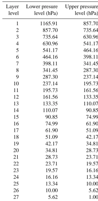
Table 1. Retrieval grid layers of GOSAT/TANSO-FTS TIR CO2V1 data.
Layer Lower presure Upper pressure
level level (hPa) level (hPa)
1 1165.91 857.70
2 857.70 735.64
3 735.64 630.96
4 630.96 541.17
5 541.17 464.16
6 464.16 398.11
7 398.11 341.45
8 341.45 287.30
9 287.30 237.14
10 237.14 195.73
11 195.73 161.56
12 161.56 133.35
13 133.35 110.07
14 110.07 90.85
15 90.85 74.99
16 74.99 61.90
17 61.90 51.09
18 51.09 42.17
19 42.17 34.81
20 34.81 28.73
21 28.73 23.71
22 23.71 19.57
23 19.57 16.16
24 16.16 13.34
25 13.34 10.00
26 10.00 5.62
27 5.62 1.00
28 1.00 0.10
2000) as
A=GKW. (2)
Figure 1 shows typical averaging kernel functions of TIR V1 L2 CO2retrieval. The degrees of freedom (DF) in these cases
(trace of the matrix A) were (a) 2.22, (b) 1.81, and (c) 1.36. The seasonally averaged DF values of TIR V1 CO2 data
ranged from 1.12 to 2.35. At the low and middle latitudes between 35◦N and 35◦S, the CO2 DF values were around
2.0 or more; this means that observations by the TIR band of TANSO-FTS can provide information on CO2
concentra-tions in more than two vertical layers, one of which we fo-cused on in this study.
A priori and initial values for CO2 concentrations were
taken from the outputs of the NIES transport model (NIES-TM05) (Saeki et al., 2013b). A priori and initial values for temperature and water vapor were obtained from Japan Me-teorological Agency (JMA) Grid Point Value (GPV) data. Basically, the retrieval processing of TANSO-FTS was only conducted under clear-sky conditions, which was judged based on a cloud flag from TANSO-CAI in the daytime
(Ishida and Nakajima, 2009; Ishida et al., 2011) and on a TANSO-FTS TIR spectrum in the nighttime.
4.2 Improvements in the TIR V1 CO2algorithm
The following conditions are the improvements made in the TANSO-FTS TIR V1 L2 CO2 algorithm from the V00.01
algorithm. The V1 algorithm used the CO2 10 µm
ab-sorption band in addition to the CO2 absorption band at
around the 15 µm band; the wavelength regions of 690– 750, 790–795, 930–990, and 1040–1090 cm−1 were used in the CO2 retrieval. We did not apply any channel
selec-tion. In these wavelength regions, temperature, water va-por, and ozone concentrations were retrieved simultaneously with CO2concentration. Moreover, surface temperature and
surface emissivity were simultaneously derived as a correc-tion parameter of the spectral bias inherent in TANSO-FTS TIR V161.160 L1B spectra at the above-mentioned CO2
absorption bands. We assumed that the spectral bias could be divided into two components: a wavelength-dependent bias whose amount varied depending on wavelength and a wavelength-independent bias whose amount was uniform in a certain wavelength region. We tried to correct such a wavelength-independent component of the spectral bias by adjusting the value of surface temperature. Similarly, a wavelength-dependent component of the spectral bias was corrected by adjusting the value of surface emissivity in each wavelength channel. Therefore the matrices of K and Sa of
expression (1) are as follows:
K= KCO2KH2OKO3KTksT_1ksT_2ksT_3ksT_4ksT_5
ksE_1ksE_2ksE_3ksE_4ksE_5, (3)
Sa=
SCO2
SH2O
SO3
ST
SsT_1
SsT_2 0
SsT_3
0 SsT_4
SsT_5
SsE_1
SsE_2
SsE_3
SsE_4
SsE_5
, (4)
where KCO2, KH2O, KO3, and KT are Jacobian matrices of
CO2, water vapor, ozone, and temperature on full grids,
re-spectively, and SCO2, SH2O, SO3, and ST are a priori
covari-ance matrices of CO2, water vapor, ozone, and temperature
on full grids, respectively. The vectorsksT_1,ksT_2,ksT_3,
ksT_4, andksT_5are the Jacobian vectors of surface
-0.1 0.0 0.1 0.2 Averaging kernel
Retrieval layer level
50 60 70 80 90 100
200
300
400 500 600 700 800 900 1000
Pressure [hPa]
-0.1 0.0 0.1 0.2 Averaging kernel
Retrieval layer level
8 12 16 20 24 28 4
-0.1 0.0 0.1 0.2 Averaging kernel
Retrieval layer level
8 12 16 20 24 28
4 4 8 12 16 20 24 28
(a) (b) (c)
Figure 1. Averaging kernel functions of GOSAT/TANSO-FTS TIR V1 CO2retrieval in the 28 retrieval grid layers shown in Table 1: (a) low latitudes in summer, (b) middle latitudes in spring, and (c) high latitudes in winter. Solid orange, yellow, and green lines indicate averaging kernel functions of each of the three layer levels: 9, 10, and 11, respectively.
vectors of surface emissivity in each of the five wavelength regions. The elements of the Jacobian vectors of surface pa-rameters that were defined for each of the five wavelength regions were set to be zero in the other wavelength regions. The values SsT_1, SsT_2, SsT_3, SsT_4, and SsT_5and SsE_1,
SsE_2, SsE_3, SsE_4, and SsE_5are a priori variances of
sur-face temperature and sursur-face emissivity in each of the five wavelength regions, respectively. Simultaneous retrieval of the surface parameters in the V1 algorithm was conducted just for the purpose of correcting the TIR V161.160 L1B spectral bias; it had no physical meaning. We estimated the surface parameters separately in each of the five wavelength regions to consider differences in the amount of spectral bias in each wavelength region. The matrices Safor CO2,
temper-ature, water vapor, and ozone were diagonal matrices with vertically fixed diagonal elements with a standard deviation of 2.5 %, 3 K, 20 %, and 30 %, respectively. Here, a priori and initial values for ozone were obtained from the clima-tological data for each latitude bin for each month given by MacPeters et al. (2007). We assumed rather large values as a priori variances of the surface parameters (a standard de-viation of 10 K for surface temperature), which could allow more flexibility in the L1B spectral bias correction by the surface parameters. The a priori and initial values for surface emissivity were calculated by linear regression analysis using the Advanced Space-borne Thermal Emission Reflection Ra-diometer (ASTER) Spectral Library (Baldridge et al., 2009) using land-cover classification, vegetation, and wind speed information. The a priori and initial values for surface tem-perature were estimated using radiance data in several chan-nels around 900 cm−1of the TIR V161.160 L1B spectra.
In the TIR V1 L2 algorithm, we estimated surface temper-ature and surface emissivity to correct the spectral bias in-herent in the TANSO-FTS TIR L1B spectra (Kataoka et al., 2014). The existence of a relatively large spectral bias around the CO2 15 µm absorption band in TANSO-FTS TIR L1B
spectra (Kataoka et al., 2014) resulted in a decrease in the number of normally retrieved CO2profiles. This is probably
because the TIR L1B spectral bias in the CO215 µm
absorp-tion band was sometimes too large for the L2 retrieval cal-culation to converse in a limited iteration. The correction of the TIR L1B spectral bias through the simultaneous retrieval of the surface parameters did not affect retrieved CO2
con-centrations in the UTLS regions, which was the focus of this study, but it altered the number of normally retrieved CO2
profiles. The correction of the TIR L1B spectral bias through the simultaneous retrieval of surface temperature increased the number of normally retrieved CO2 profiles. This
im-plies that a wavelength-independent component of the spec-tral bias in CO2absorption bands could be reduced by
ad-justing the value of surface temperature at the bands. In con-trast, the spectral bias correction through the simultaneous retrieval of surface emissivity did not increase the number of normally retrieved CO2profiles. If the TIR L1B spectral bias
has a wavelength dependence, surface emissivity could be effective for correcting such a wavelength-dependent bias. A more effective method of L1B spectral bias correction based on surface emissivity should be considered in the next ver-sion of the TIR L2 CO2 retrieval algorithm if a future
0˚ 0˚
60˚ 60˚
120˚ 120˚
180˚ 180˚
−120˚ −120˚
−60˚ −60˚
−90˚ −90˚
−60˚ −60˚
−30˚ −30˚
0˚ 0˚
30˚ 30˚
60˚ 60˚
90˚ 90˚
1 3 2 4
12 5 8 9 10 11
13 6
14 7
15
21 16
1718 19
20
36
25
22 23 26
27 28 29 30 31
33 32
38 37
34
24
35
40 39
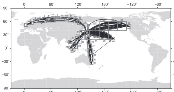
Figure 2. Flight tracks of all of the CONTRAIL CME observations in 2010 used in this study. The number next to each box area indicates its area number.
5 Comparison methods
5.1 Area comparisons
Here, we used the level flight CO2 data of CONTRAIL
CME observations in 2010 to validate the quality of UTLS CO2 data from the TANSO-FTS TIR V1 L2 CO2
product. The level flight data obtained from the follow-ing eight airline routes of the CONTRAIL CME ob-servations were used in this study: Tokyo–Amsterdam (NRT–AMS) and Tokyo–Moscow (NRT–DME), Tokyo– Vancouver (NRT–VYR), Tokyo–Honolulu (NRT–HNL), Tokyo–Bangkok (NRT–BKK), Tokyo–Singapore (NRT– SIN) and Tokyo–Jakarta (NRT–CGK), and Tokyo–Sydney (NRT–SYD). We merged the level flight data of Tokyo– Amsterdam and Tokyo–Moscow into “Tokyo–Europe”, and the data of Tokyo–Singapore and Tokyo–Jakarta into “Tokyo–East Asia”. Figure 2 shows the flight tracks of all of the CONTRAIL CME observations in 2010 used in this study. As shown in the figure, we divided the CON-TRAIL CME level flight data into 40 areas following Niwa et al. (2012), and compared them with TANSO-FTS TIR CO2
data in each area in each season. The amount of level flight data varied depending on the area and season. The largest amount of data was obtained in area 15 over Narita Air-port, where 4694–9306 data points were obtained. A rela-tively small amount of level flight data, 79–222 data points, was obtained in area 1 over Amsterdam. In all 40 areas, we collected sufficient level flight data to undertake comparison analysis based on the average values, except for seasons and regions with no flights.
5.2 Comparisons of CME profiles with and without averaging kernels
In comparisons of TIR V1 L2 CO2 data with the
CON-TRAIL CME level flight data, it is difficult to smooth the CME data by applying TIR CO2averaging kernels, because
CO2 concentrations below and above the CME flight levels
were not observed. Here, we evaluated the impact of con-sidering averaging kernel functions on CO2 concentrations
using the CME profile data. We regarded the CME data ob-tained during the ascent and descent flights over the nine air-ports as part of CO2 vertical profiles, and investigated
dif-ferences between TIR and CME CO2data with and without
applying averaging kernel functions in the altitude regions around the CME level flight observations. We assumed the CME ascending/descending CO2concentration at the
upper-most altitude level to be constant up to the tropopause height, following the method proposed by Araki et al. (2010). We used stratospheric CO2data taken from the Nonhydrostatic
Icosahedral Atmospheric Model (NICAM)–Transport Model (TM) (Niwa et al., 2011, 2012) to create whole CO2
ver-tical profiles over the airports. The NICAM-TM CO2 data
used here introduced CONTRAIL CO2 data to the inverse
model in addition to surface CO2data, and therefore could
simulate upper-atmospheric CO2concentrations well (Niwa
et al., 2012). We determined the stratospheric CO2 profile
by assuming the CO2concentration gradients, calculated on
the basis of the NICAM-TM CO2data above the tropopause
height.
To compare these CME CO2profiles with TIR CO2data,
we calculated a weighted average of all the CME CO2data
included in each of the 28 retrieval grid layers with respect to altitude, and defined the CO2 data in the 28 layers as
“CONTRAIL (raw)” data. Then, we selected TIR CO2data
from Narita airport, and a 3-day difference of each other ob-servation. We applied TIR CO2 averaging kernel functions
to the corresponding CONTRAIL (raw) profile, as follows (Rodgers and Connor, 2003):
xCONTRAIL (AK)=xa priori+A xCONTRAIL (raw)−xa priori
. (5)
Here, xCONTRAIL (raw) and xa priori are CONTRAIL (raw)
and a priori CO2profiles. We defined the CONTRAIL (raw)
data with TIR CO2 averaging kernel functions as
“CON-TRAIL (AK)” data.
5.3 Level flight comparisons
In this study, we made comparisons between TIR and CON-TRAIL CME level flight CO2 data in two ways. The first
was a direct comparison with original CME CO2data, i.e.,
CONTRAIL (raw) data. The second was a comparison with CONTRAIL (AK) data in the altitude regions around the CME level flight observations that were based on “assumed CO2profiles” created at each of the measurement locations
of all the CME level flight data. In the first comparison with CONTRAIL (raw) data, the CME level flight data in each of the 40 areas were averaged for each season (MAM, JJA, SON, and JF/DJF). The average altitude of all of the CME level flight data used here was 11.245 km. The airline routes of Tokyo–Europe, Tokyo–Vancouver, and Tokyo–Honolulu contained both tropospheric and stratospheric data in the ar-eas along their routes; therefore, we calculated the average and standard deviation values separately. Here, we differen-tiated between the tropospheric and stratospheric level flight data on the basis of temperature lapse rates from the JMA GPV data that were interpolated to the CONTRAIL CME measurement locations. The average altitudes of the tropo-spheric and stratotropo-spheric level flight data from the airline route between Tokyo and Europe were 10.84 and 11.18 km, respectively.
In the comparison with CONTRAIL (raw) data, we se-lected TANSO-FTS TIR V1 L2 CO2 data that were in the
altitude range within ±1 km of the average altitude of the CME level flight data for each area for each season, and we calculated their averages and standard deviations. Similarly, we calculated the averages and standard deviations of the cor-responding a priori CO2data for each area for each season.
For the airline routes of Tokyo–Europe, Tokyo–Vancouver, and Tokyo–Honolulu, the averages and standard deviations of TIR V1 CO2data and the corresponding a priori CO2data
were calculated separately for the tropospheric and strato-spheric data. In this calculation, we first selected TIR V1 CO2 data that were collected in a range within ±1 km of
the average altitudes of the CONTRAIL tropospheric and stratospheric CO2 data for each area. Then, we classified
each of the selected TIR CO2 data points into tropospheric
and stratospheric data on the basis of the temperature lapse rates from the JMA GPV data that were interpolated to the TANSO-FTS measurement locations, and we calculated the
0 5000 10 000 15 000 20 000 25 000
Level 8 Level 9 Level 10 Level 11
N
um
be
r of
da
ta
poi
nt
s
Retrieval layer level
NRT_DME_AMS T
NRT_DME_AMS S
NRT_YVR T
NRT_YVR S
NRT_HNL T
NRT_HNL S
NRT_BKK
NRT_SIN_CGK
NRT_SYD
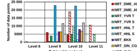
Figure 3. The number of GOSAT/TANSO-FTS TIR CO2 data
points compared to the CONTRAIL CME level flight data for each retrieval grid layer level for each flight. The num-bers of TIR CO2 data points in the troposphere (“T”) and stratosphere (“S”) are shown separately for the Tokyo–Europe (NRT_DME_AMS), Tokyo–Vancouver (NRT_YVR), and Tokyo– Honolulu (NRT_HNL) flight routes.
seasonal averages and standard deviations for the reselected tropospheric and stratospheric TIR CO2data. This procedure
was required for two reasons: (1) tropopause height at each TANSO-FTS measurement location should differ on a daily basis, and (2) because TIR CO2 data were selected within
the range of 2 km, some tropospheric TIR CO2 data were
selected on the basis of the CONTRAIL stratospheric level flight data, and vice versa. Figure 3 shows the number of TANSO-FTS TIR CO2data points that were finally selected
in each retrieval layer for each of the airline routes. The TIR CO2data used in the comparative analysis were mainly from
layers 9 and 10 (from 287 to 196 hPa) for the tropospheric comparison and from layers 10 and 11 (from 237 to 162 hPa) for the stratospheric comparison.
In the second comparison, we assumed a CO2 vertical
profile on the basis of CONTRAIL (raw) data at each of the CONTRAIL CME level flight locations and applied TIR CO2averaging kernel functions to the assumed profiles. For
this purpose, realistic CO2 vertical profiles were required
along the eight airline routes. In this study, we created a CO2profile at each CME level flight measurement location
from CarbonTracker CT2013B monthly-mean CO2data
(Pe-ters et al., 2007). The CarbonTracker CT2013B CO2data are
available to the public, and therefore readers can refer to the data set that we used as a CO2climatological data set. The
method for creating a CO2 vertical profile from the
CON-TRAIL (raw) and CarbonTracker CT2013B data is as fol-lows. We first averaged all of the CarbonTracker CT2013B monthly-mean data included in each of the 40 areas to cre-ate area-averaged CarbonTracker CT2013B profiles. Then, we shifted the area-averaged CarbonTracker CT2013B pro-file so that its concentration fit to each of the CONTRAIL (raw) data at CME level flight altitude. Finally, we applied area-averaged TIR CO2averaging kernel functions to each of
the shifted area-averaged CO2profiles and created profiles of
We compared the CONTRAIL (AK) data with TIR CO2
data at the altitude regions around the CME level flight ob-servations for each area in each season. We extracted CON-TRAIL (AK) data that corresponded to the TIR retrieval layers where TIR CO2data were compared to CONTRAIL
(raw) data, and we averaged them for each area for each season. For the airline routes of Tokyo–Europe, Tokyo– Vancouver, and Tokyo–Honolulu, we separately averaged CONTRAIL (AK) data created from tropospheric and strato-spheric CONTRAIL (raw) data and defined the averages as tropospheric and stratospheric CONTRAIL (AK) data, re-spectively. As shown in Fig. 3, the CONTRAIL (AK) data used for the comparison during flights between Tokyo and Sydney consisted of CO2concentrations in layers 9 and 10 of
the CONTRAIL (AK) profiles. For the flights between Tokyo and Europe, the CONTRAIL (AK) data used for the tropo-spheric and stratotropo-spheric comparisons were based on CO2
concentrations in layers 9 and 10 and in layers 10 and 11 of CONTRAIL (AK) profiles, respectively.
6 Comparison results
6.1 Impacts of averaging kernels on CME profiles
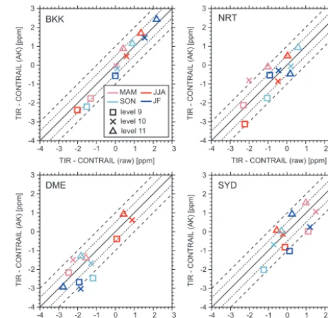
Figure 4 shows comparisons of the differences between TANSO-FTS TIR and CONTRAIL (raw) CO2data, and the
differences between TIR and CONTRAIL (AK) CO2 data
at low (BKK), middle (NRT and SYD), and high (DME) latitudes in layers 9, 10, and 11. At low latitudes, the dif-ferences between CONTRAIL (raw) and CONTRAIL (AK) were mostly less than 0.5 ppm in all seasons. This is be-cause the tropopause heights there were much higher than the altitude levels of CONTRAIL CME level flight measure-ments, and CO2concentrations did not change much in the
altitude regions where we compared TIR and CONTRAIL CME data. The same was true for other airports at low lati-tudes. While the differences between CONTRAIL (raw) and CONTRAIL (AK) were larger at middle and high latitudes than at low latitudes, they were in most cases less than 1 ppm in all seasons. In conclusion, the impact of applying the TIR CO2 averaging kernels on CONTRAIL CME CO2 data at
around the CME level flight altitudes (∼11 km) was on av-erage less than 0.5 ppm at low latitudes and less than 1 ppm at middle and high latitudes.
6.2 Comparisons during level flight
The airline route between Tokyo and Sydney covered a wide latitude range from the northern middle latitudes (35◦N) to southern middle latitudes (34◦S). Figure 5 shows comparisons among CONTRAIL (raw), CONTRAIL (AK), TANSO-FTS TIR, and a priori CO2data during flights
be-tween Tokyo and Sydney in northern hemispheric spring. In this case, we averaged CO2 data mainly from layers 9 and
10 of the TIR retrieval layer levels. The 1σ values of the
av-DME
NRT
SYD
JJA SON
level 10 level 9 MAM
JF
level 11 -4
-3 -2 -1 0 1 2 3
TIR - CONTRAIL (AK) [ppm]
-4 -3 -2 -1 0 1 2 3
TIR - CONTRAIL (raw) [ppm]
BKK
-4 -3 -2 -1 0 1 2 3
TIR - CONTRAIL (AK) [ppm]
-4 -3 -2 -1 0 1 2 3
TIR - CONTRAIL (raw) [ppm]
-4 -3 -2 -1 0 1 2 3
TIR - CONTRAIL (AK) [ppm]
-4 -3 -2 -1 0 1 2 3
TIR - CONTRAIL (raw) [ppm]
-4 -3 -2 -1 0 1 2 3
TIR - CONTRAIL (AK) [ppm]
-4 -3 -2 -1 0 1 2 3
TIR - CONTRAIL (raw) [ppm]
Figure 4. Scatterplots of GOSAT/TANSO-FTS TIR and
CON-TRAIL (raw) CO2differences and GOSAT/TANSO-FTS TIR and
CONTRAIL (AK) CO2differences in layers 9, 10, and 11 for each season.
384 386 388 390 392
CO
2
[ppm]
Latitude
-40 -30 -20 -10 0 10 20 30 40
CONTRAIL (raw) TIR A priori CONTRAIL (AK)
Figure 5. Comparisons among CONTRAIL (raw), CONTRAIL (AK), GOSAT/TANSO-FTS TIR, and a priori (NIES TM 05) CO2 data during flights between Tokyo and Sydney (NRT_SYD) in northern hemispheric spring (MAM), shown by black, gray, red, and green lines, respectively. The means and their 1σstandard de-viations were calculated in each area during the flight for all four data sets.
erages show the variability of CO2 concentrations in these
UTLS layers. The average of the TIR CO2data agreed
bet-ter with the averages of the CONTRAIL (raw) and (AK) CO2data than the a priori CO2data at all latitudes. The
CO
2
[ppm]
(a) (b) (c)
384 386 388 390 392
Longitude
105 120 135 150
0 15 30 45 60 75 90
Longitude
105 120 135 150
0 15 30 45 60 75 90
Longitude
105 120 135 150
0 15 30 45 60 75 90
CONTRAIL (raw) TIRA priori CONTRAIL (AK)
Figure 6. Same as Fig. 5 but for flights between Tokyo and Europe (NRT_DME_AMS) in winter (JF). (a) All of the data, (b) only data in the troposphere, and (c) only data in the stratosphere. See the text for the classification of tropospheric and stratospheric data.
monthly-mean data. In the Southern Hemisphere, the aver-age of the TIR CO2data was within 0.1 % of the averages of
the CONTRAIL (raw) and CONTRAIL (AK) CO2data. In
the Northern Hemisphere, the average of the TIR CO2data
agreed with the averages of the CONTRAIL (raw) and CON-TRAIL (AK) CO2data to within 0.5 %, although the
agree-ment was slightly worse there than in the Southern Hemi-sphere.
Along the airline route between Tokyo and Europe, both tropospheric and stratospheric CO2 data were obtained in
the CONTRAIL CME observations. Therefore, we were able to validate the quality of TANSO-FTS TIR CO2 data for
this route both in the upper troposphere and lower strato-sphere using the UTLS CME CO2 data. Here, we
aver-aged CO2data mainly from layers 9 and 10 for the
upper-tropospheric comparison and from layers 10 and 11 for the lower-stratospheric comparison. As shown in Fig. 6, the dif-ferences between CONTRAIL (raw) and CONTRAIL (AK) were again approximately 0.5 ppm when CONTRAIL CME data were divided into the upper troposphere and lower stratosphere, which is consistent with the result shown in Fig. 4. Figure 6b and c shows that the differences between the upper-tropospheric and lower-stratospheric CO2
concen-trations of CONTRAIL CME data were approximately 2– 3 ppm in winter (maximum of 4.24 ppm in area 14). The upper-tropospheric and lower-stratospheric CO2
concentra-tions from TANSO-FTS TIR V1 data also clearly differed, while the upper-tropospheric and lower-stratospheric CO2
concentrations from a priori data were similar. The upper-tropospheric TIR CO2concentrations were in a good
agree-ment within 1 ppm with the corresponding CONTRAIL (raw) and CONTRAIL (AK) data (Fig. 6b). In the lower stratosphere in winter (Fig. 6c), the averages of the CON-TRAIL (raw), CONCON-TRAIL (AK), TANSO-FTS TIR, and a priori CO2data were all within 0.5–1 ppm of each other.
Figure 7 shows the results of all of the comparisons among CONTRAIL (raw), CONTRAIL (AK), TANSO-FTS TIR, and a priori CO2 data in the upper troposphere (left) and
lower stratosphere (right) for each season. We divided the
data for all four data sets in each of the 40 areas into six lat-itude bands: 40–20◦S (areas 30 and 31), 20–0◦S (areas 21, 28, and 29), 0–20◦N (areas 16, 17, 20, 22, 23, 26, and 27), 20–40◦N (areas 15, 18, 19, 24, 25, and 37–40), 40–60◦N (areas 1, 2, 14, and 32–36), and 60–70◦N (areas 3–13). As for the lower stratosphere, we showed the results at northern latitudes of 40◦N where an adequate amount of data was ob-tained. Overall, the black and gray lines (TIR average minus CONTRAIL (raw) average, and TIR average minus CON-TRAIL (AK) average) were closer to zero than the green lines (a priori average minus CONTRAIL (raw) average), which means that TIR CO2 data agreed better with
CON-TRAIL CME CO2data than a priori CO2data.
The left panels of Fig. 7 show that the agreements between TIR and CONTRAIL (raw) and CONTRAIL (AK) CO2
av-erage data were worse in spring and summer than in fall and winter in the Northern Hemisphere in the upper troposphere. The differences between TIR and CONTRAIL (raw) and CONTRAIL (AK) CO2data were on average within 1 ppm
in fall and winter in the northern troposphere. At 0–40◦N in summer, in contrast, the TIR and a priori CO2average data
were 2.3 ppm lower than the CONTRAIL (AK) CO2average
data. At 20–40◦N in spring, the differences between TIR and CONTRAIL (AK) CO2average data were 2.4 ppm, although
the TIR CO2data had a better agreement with CONTRAIL
CME CO2data than a priori CO2data. On the other hand, the
averages of the TIR CO2data were within 0–0.7 ppm of the
averages of the CONTRAIL (AK) CO2data in the Southern
Hemisphere in all seasons, as in the comparison in northern hemispheric spring shown in Fig. 5.
In the lower stratosphere, the agreements between the av-erage TANSO-FTS TIR and CONTRAIL CME CO2data did
not have a smaller seasonality than in the upper troposphere. The averages of TIR and CONTRAIL (raw) and CONTRAIL (AK) CO2 data agreed with each other within 0.5 % in all
-4 -3 -2 -1 0 1 2 3 CO 2
ave. difference [ppm]
Latitude
-40 -20 0 20 40 60
-4 -3 -2 -1 0 1 2 3 CO 2
ave. difference [ppm]
Latitude
-40 -20 0 20 40 60
-4 -3 -2 -1 0 1 2 3 CO 2
ave. difference [ppm]
Latitude
-40 -20 0 20 40 60
-4 -3 -2 -1 0 1 2 3 CO 2
ave. difference [ppm]
Latitude
-40 -20 0 20 40 60
MAM JJA SON JF T T T T S S S S 40 60 Latitude -4 -3 -2 -1 0 1 2 3 40 60 Latitude -4 -3 -2 -1 0 1 2 3 40 60 Latitude -4 -3 -2 -1 0 1 2 3 40 60 Latitude -4 -3 -2 -1 0 1 2 3
Figure 7. Differences between GOSAT/TANSO-FTS TIR and CONTRAIL (raw) averaged CO2data (TIR average minus CON-TRAIL (raw) average), TIR and CONCON-TRAIL (AK) averaged CO2 data (TIR average minus CONTRAIL (AK) average), and a priori (NIES TM 05) and CONTRAIL (raw) averaged CO2data (a priori average minus CONTRAIL (raw) average) for each season for each latitude band (40–20◦S, 20–0◦S, 0–20◦N, 20–40◦N, 40–60◦N, 60–70◦N), shown by black, gray, and green lines, respectively. Left and right panels show the differences in the upper troposphere and lower stratosphere, respectively. The 1σ standard deviations of the latitudinal averages of TANSO-FTS TIR CO2data are shown by vertical bars.
7 Discussion
As shown in Fig. 7, TANSO-FTS TIR V1 L2 CO2data had a
negative bias of 2.3–2.4 ppm against CONTRAIL CME CO2
data at the northern low and middle latitudes in spring and summer. Uncertainties in surface parameters and temperature profiles could affect CO2retrieval in thermal infrared
spec-tral regions. As described above, retrieving surface ters simultaneously instead of using initial surface parame-ters did not affect CO2concentrations in the UTLS regions
in the TIR V1 CO2retrieval. We compared simultaneously
retrieved temperature profiles with a priori JMA GPV tem-perature profiles in the UTLS region and did not find any dif-ference between the two which could explain the largest TIR CO2negative bias at the northern low and middle latitudes in
spring and summer. In the UTLS regions, temperature vari-ability is relatively large, and therefore comprehensive vali-dation analysis of both the a priori and retrieved temperature profiles should be required using reliable and independent temperature data such as radiosonde data.
Uncertainty in a priori data could result in uncertainty in retrieved CO2data. Here, we arbitrarily decreased the a
pri-ori concentration by 1 % in a test TIR CO2retrieval and then
compared the retrieved CO2 concentrations with those
re-trieved using the original a priori data. At the northern low and middle latitudes in spring and summer where the DF values of TIR V1 CO2 data were around 1.8 and more, a
1 % negative bias in a priori data could yield up to a 0.7 % negative bias in retrieved CO2concentrations in the altitude
regions where we did comparisons between TIR and CON-TRAIL CME data, although the magnitude of the bias varied depending on retrievals. As shown by the green lines in Fig-ure 7, a priori CO2 concentrations were underestimated by
2–4 ppm at the northern low and middle latitudes in spring and summer. The test TIR CO2 retrieval demonstrated that
the negative bias of a priori CO2 data against CONTRAIL
CME data is a possible cause of the TIR CO2negative bias
in the UTLS regions at the northern low and middle latitudes in spring and summer.
In general, the information content of CO2 observations
made by TIR sensors is higher at middle and high latitudes in spring and summer than in fall and winter because of the thermal contrast in the atmosphere, with less seasonal depen-dence at low latitudes. Therefore, in spring and summer, re-trieved CO2data contain more measurement information and
are less constrained by a priori data at all latitudes. However, as shown in Fig. 7, the retrieved TIR CO2data at the
north-ern low and middle latitudes did not sufficiently reduce the negative bias of the a priori CO2 data in the UTLS regions
in spring and summer. This implies the existence of factors that worsened CO2 retrieval results other than the a priori
data, especially in spring and summer. Another possible fac-tor that worsened CO2retrieval results is the uncertainty in
the calibration of TIR V161.160 L1B spectra. As reported in Kataoka et al. (2014), TANSO-FTS TIR V130.130 L1B radi-ance spectra had a wavelength-dependent bias ranging from 0.1 to 2 K. Although the characteristics of the spectral bias in V161.160 L1B data used in TIR V1 L2 CO2retrievals are
equation:
dCO2 =GCO2dspec. (6)
Here, GCO2 is a gain matrix for CO2 retrieval, dspec is a
spectral bias vector based on the evaluation by Kataoka et al. (2014), and dCO2 is a vector of bias errors in retrieved
CO2concentrations attributable to the spectral bias. The
re-sult showed that a wavelength-dependent bias comparable to V130.130 L1B spectra could yield up to 0.3 and 0.5 % uncer-tainties in retrieved CO2concentration in the UTLS regions
at the northern middle latitude in spring and at the north-ern low latitude in summer, respectively. Uncertainty in the radiometric calibration of TANSO-FTS L1B spectra causes the spectral bias inherent in TIR L1B spectra. The tempera-tures of the internal blackbody on board the TANSO-FTS in-strument partly reflect the environmental thermal conditions inside the instrument. The temperatures of FTS mechanics and aft optics on the optical bench of the TANSO-FTS in-strument are precisely controlled at 23◦C. The difference in temperature between the environment inside the instrument and the optical bench could cause the uncertainty in the ra-diometric calibration of TANSO-FTS L1B spectra. Thus, the temperatures of the internal blackbody on board the TANSO-FTS instrument could be a parameter used to evaluate the TANSO-FTS TIR L1B spectral bias.
Figure 8 shows the averages of the partial degree of free-dom of TANSO-FTS TIR V1 L2 CO2 data for each of the
areas along the airline routes between Tokyo and Europe in the upper troposphere (a) and the lower stratosphere (b) for each season. The partial DF is defined as the diagonal el-ement of the averaging kernels corresponding to TIR CO2
data that were compared to CONTRAIL CME level flight data, which is equal to the 9th, 10th, or 11th diagonal ele-ment of matrix A. As shown in Fig. 8, the average values of the partial DF of TIR lower-stratospheric CO2data were
clearly lower than those of TIR upper-tropospheric CO2data
for all of the fights between Tokyo and Europe. TIR upper-tropospheric CO2data were from layers 9 and 10, and TIR
lower-stratospheric CO2 data were from layers 10 and 11,
as shown in Fig. 3, which led to a clear difference in partial DF values between the TIR upper-tropospheric and lower-stratospheric CO2data. The partial DF values of TIR
upper-tropospheric CO2data were 0.13–0.20 in all of the areas for
all seasons. In contrast, the partial DF values of TIR lower-stratospheric CO2data in spring, fall, and winter were∼0.05
in almost all of the areas, although they were as high as 0.1– 0.14 in summer. From the results shown in Figs. 6c and 8, we conclude that TIR CO2 retrieval results in the lower
strato-sphere in winter were constrained to the relatively good a pri-ori CO2data due to the low information content and
conse-quently had a good agreement with CONTRAIL CME CO2
data. The comparisons in the areas during the airline route between Tokyo and Europe were included in the compari-son results of 60–70◦N in the right panels of Fig. 7. In this
Longitude
105 120 135 150 90
60
30 45 75
15 0 0.00 0.05 0.10 0.15 0.20 0.25
Partial DF
0.00 0.05 0.10 0.15 0.20 0.25
Partial DF
MAM
JJA SONJF
(a)
(b)
Figure 8. Partial degree of freedom (DF) for GOSAT/TANSO-FTS TIR CO2data in the upper troposphere (a) and the lower strato-sphere (b) for each area of the flight between Tokyo and Europe (NRT_DME_AMS). The means and their 1σ standard deviations of the partial DF data were calculated in spring (MAM), summer (JJA), fall (SON), and winter (JF), as shown by the pink, red, light blue, and blue lines, respectively.
region, the average differences between a priori and CON-TRAIL (raw) data were 1–2 ppm in summer and fall, while they were less than 0.5 ppm in spring and winter. In summer, TIR CO2retrievals had a relatively high information content
compared to the other seasons, which led to an agreement between TIR and CONTRAIL (raw) and CONTRAIL (AK) CO2 data of within 0.5 ppm. In fall, TIR CO2 retrieval
re-sults in the lower stratosphere were more constrained to the a priori CO2 data and therefore had a negative bias of
ap-proximately 1–2 ppm against CONTRAIL (raw) and CON-TRAIL (AK) CO2 data. In conclusion, the quality of TIR
V1 CO2 data in the lower stratosphere depends largely on
the information content compared to the upper troposphere. In the case of high-latitude measurements, TIR V1 lower-stratospheric CO2data are only valid in summer.
We investigated the differences between TIR and CON-TRAIL CO2 comparison results in layers 9–11 with and
without applying averaging kernel functions over the nine airports where CO2 vertical profiles were observed during
mid-Table 2. Bias values of GOSAT/TANSO-FTS TIR V1 CO2data against CONTRAIL (AK) CO2data for each season and each latitude region in the upper troposphere and lower stratosphere in units of parts per million (ppm). Significant bias values larger than±2 ppm are indicated by boldface.
UT LS MAM JJA SON JF
60–70◦N −1.0 −0.8 −0.2 −0.5 −1.0 −1.1 0.3 −0.5
40–60◦N −1.7 0.3 −1.6 −1.3 −1.1 −0.9 −0.5 −0.5
20–40◦N −2.4 −2.3 −1.1 0.3
0–20◦N −1.2 −2.3 −0.5 0.5
20–0◦S −0.1 −0.6 0.4 0.0
40–20◦S −0.2 −0.4 −0.7 −0.5
dle latitudes in spring (SYD in Fig. 4); CONTRAIL (AK) was on average 1.1 and 0.4 ppm higher than CONTRAIL (raw) in layers 9 and 10. This means that CO2
concentra-tions in layers 9 and 10 were more affected by stratospheric air with relatively low CO2 concentrations at the northern
middle latitude in spring, when considering averaging ker-nels. This is consistent with the result of Sawa et al. (2012) showing that the difference between upper-tropospheric and lower-stratospheric CO2 concentrations was larger in the
Northern Hemisphere in spring.
Using CONTRAIL CME level flight observations that covered wide spatial areas allowed us to discuss the longi-tudinal differences in the characteristics of TIR UTLS CO2
data. In the comparison results of the airline routes of Tokyo– Europe (Fig. 6) and Tokyo–Vancouver (not shown here), the magnitudes of the differences between TIR and CON-TRAIL (raw) and (AK) CO2 data did not have a clear
lon-gitudinal dependence. Table 2 summarizes the latitudinal de-pendence of the magnitudes of the differences between TIR and CONTRAIL (AK) CO2data. In the upper troposphere
within 0–60◦N, negative biases in TIR CO2 data against
CONTRAIL CME CO2 data ranged from 1.2 to 2.4 ppm
in spring and summer when applying averaging kernels to the assumed CME CO2 profiles created based on
Carbon-Tracker CT2013B monthly-mean profiles. It is the negative biases at the northern low and middle latitudes that we should in particular be concerned about when using TIR V1 L2 CO2data in any scientific analysis. In the upper troposphere
at the northern middle latitudes, CO2 concentrations reach
the maximum from spring through early summer. The neg-ative biases in TIR CO2data resulted in the maximum TIR
CO2concentrations being lower than that of the CONTRAIL
CME CO2concentrations, which led to an underestimate of
the amplitude of the CO2seasonal variation when using TIR
CO2data without taking their negative biases into account.
8 Summary
In this study, we conducted a comprehensive validation of the UTLS CO2 concentrations from the
GOSAT/TANSO-FTS TIR V1 L2 CO2 product. The TIR V1 L2 CO2
algo-rithm used both the CO2 10 and 15 µm absorption bands
(690–750, 790–795, 930–990, and 1040–1090 cm−1)and si-multaneously retrieved vertical profiles of CO2, water vapor,
ozone, and temperature in these wavelength regions. Because the TANSO-FTS TIR V161.160 L1B radiance data used in the TIR V1 L2 CO2retrieval had a spectral bias, we
simul-taneously derived surface temperature and surface emissivity in the same wavelength regions as a corrective parameter, other than temperature and gas profiles, to correct the spec-tral bias. The simultaneous retrieval of surface temperature greatly increased the number of normally retrieved CO2
pro-files.
To validate the quality of TIR V1 upper-atmospheric CO2 data, we compared them with the level flight CO2
data of CONTRAIL CME observations along the fol-lowing airline routes in 2010: Tokyo–Europe (Amsterdam and Moscow), Tokyo–Vancouver, Tokyo–Honolulu, Tokyo– Bangkok, Tokyo–East Asia (Singapore and Jakarta), and Tokyo–Sydney. For the CONTRAIL data obtained during the northern high-latitude flights, we made comparisons among CONTRAIL, TIR, and a priori CO2 data separately in the
upper troposphere and in the lower stratosphere. The TIR upper-tropospheric and lower-stratospheric CO2 data that
were compared were mainly from layers 9 and 10 (287– 196 hPa) and from layers 10 and 11 (237–162 hPa), respec-tively. In this study, we evaluated the impact of considering TIR CO2averaging kernel functions on CO2concentrations
using the CME profile data over the nine airports; the impact at around the CME level flight altitudes (∼11 km) was on av-erage less than 0.5 ppm at low latitudes and less than 1 ppm at middle and high latitudes.
In the Southern Hemisphere, the averages of TANSO-FTS TIR V1 upper-atmospheric CO2 data were within 0.1 % of
the averages of CONTRAIL CO2 data with and without
TIR CO2averaging kernels for all seasons, from the limited
comparisons made during flights between Tokyo and Syd-ney, while TIR CO2data had a better agreement with
CON-TRAIL CO2 data than a priori CO2 data, with the
agree-ment being on average within 0.5 % in the Northern Hemi-sphere. The northern high-latitude comparisons suggest that the quality of TIR lower-stratospheric CO2 data depends
lower-stratospheric CO2data are only valid in summer, when
their information content is highest. Overall, the agreements of TIR and CONTRAIL CME CO2data were worse in spring
and summer than in fall and winter in the Northern Hemi-sphere in the upper tropoHemi-sphere. TIR CO2data had a
nega-tive bias up to 2.4 ppm against CONTRAIL CO2data with
TIR CO2 averaging kernels at the northern low and middle
latitudes in spring and summer. This is partly because of the larger negative bias in the a priori CO2 data. The spectral
bias inherent to TANSO-FTS TIR L1B radiance data could cause a negative bias in retrieved CO2concentrations,
partic-ularly in summer. TIR sensors can make more observations than SWIR sensors. When using the TIR UTLS CO2data,
the seasonally and regionally dependent negative biases of the TIR V1 L2 CO2data presented here should be taken into
account.
Data availability
GOSAT/TANSO-FTS TIR and a priori CO2 data and TIR
CO2 averaging kernel data are provided at http://www.
gosat.nies.go.jp/en/. Contact the CONTRAIL project (http:// www.cger.nies.go.jp/contrail/index.html) to access the CON-TRAIL CME CO2 data. CarbonTracker CT2013B and
up-dated results are provided at http://carbontracker.noaa.gov.
Acknowledgements. We thank all of the members of the GOSAT
Science Team and their associates. We are also grateful to the engineers of Japan Airlines, the JAL Foundation, and JAMCO Tokyo for supporting the CONTRAIL project. We thank Y. Niwa for providing the outputs of NICAM-TM CO2 simulations. We thank T. Saeki and S. Maksyutov for providing information on the a priori data set. CarbonTracker CT2013B results were provided by NOAA Earth System Research Laboratory (ESRL), Boulder, Colorado, USA, from the website at http://carbontracker.noaa.gov. This study was supported by the Green Network of Excellence (GRENE-ei) of the Ministry of Education, Culture, Sports, and Technology. This study was performed within the framework of the GOSAT Research Announcement.
Edited by: H. Worden
References
Araki, M., Morino, I., Machida, T., Sawa, Y., Matsueda, H., Ohyama, H., Yokota, T., and Uchino, O.: CO2column-averaged volume mixing ratio derived over Tsukuba from measurements by commercial airlines, Atmos. Chem. Phys., 10, 7659–7667, doi:10.5194/acp-10-7659-2010, 2010.
Bakwin, P. S., Tans, P. P., Hurst, D. F., and Zhao, C.: Measure-ments of carbon dioxide on very tall towers: results of the NOAA/CMDL program, Tellus, 50B, 401–415, 1998.
Baldridge, A. M., Hook, S. J., Grove, C. I., and Rivera, G.: The ASTER spectral library version 2.0, Remote Sens. Environ., 113, 711–715, doi:10.1016/j.rse.2008.11.007, 2009.
Barkley, M. P., Frieß, U., and Monks, P. S.: Measuring atmospheric CO2 from space using Full Spectral Initiation (FSI) WFM-DOAS, Atmos. Chem. Phys., 6, 3517–3534, doi:10.5194/acp-6-3517-2006, 2006.
Basu, S., Guerlet, S., Butz, A., Houweling, S., Hasekamp, O., Aben, I., Krummel, P., Steele, P., Langenfelds, R., Torn, M., Biraud, S., Stephens, B., Andrews, A., and Worthy, D.: Global CO2fluxes estimated from GOSAT retrievals of total column CO2, Atmos. Chem. Phys., 13, 8695–8717, 2013.
Basu, S., Krol, M., Butz, A., Clerbaux, C., Sawa, Y., Machida, T., Matsueda, H., Frankenberg, C., Hasekamp, O. P., and Aben, I.: The seasonal variation of the CO2flux over Tropical Asia es-timated from GOSAT, CONTRAIL, and IASI, Geophys. Res. Lett., 41, 1809–1815, 2014.
Brenninkmeijer, C. A. M., Crutzen, P., Boumard, F., Dauer, T., Dix, B., Ebinghaus, R., Filippi, D., Fischer, H., Franke, H., Frieß, U., Heintzenberg, J., Helleis, F., Hermann, M., Kock, H. H., Koep-pel, C., Lelieveld, J., Leuenberger, M., Martinsson, B. G., Miem-czyk, S., Moret, H. P., Nguyen, H. N., Nyfeler, P., Oram, D., O’Sullivan, D., Penkett, S., Platt, U., Pupek, M., Ramonet, M., Randa, B., Reichelt, M., Rhee, T. S., Rohwer, J., Rosenfeld, K., Scharffe, D., Schlager, H., Schumann, U., Slemr, F., Sprung, D., Stock, P., Thaler, R., Valentino, F., van Velthoven, P., Waibel, A., Wandel, A., Waschitschek, K., Wiedensohler, A., Xueref-Remy, I., Zahn, A., Zech, U., and Ziereis, H.: Civil Aircraft for the reg-ular investigation of the atmosphere based on an instrumented container: The new CARIBIC system, Atmos. Chem. Phys., 7, 4953–4976, doi:10.5194/acp-7-4953-2007, 2007.
Buchwitz, M., de Beek, R., Burrows, J. P., Bovensmann, H., Warneke, T., Notholt, J., Meirink, J. F., Goede, A. P. H., Bergam-aschi, P., Körner, S., Heimann, M., and Schulz, A.: Atmospheric methane and carbon dioxide from SCIAMACHY satellite data: initial comparison with chemistry and transport models, Atmos. Chem. Phys., 5, 941–962, doi:10.5194/acp-5-941-2005, 2005. Butz, A., Guerlet, S., Hasekamp, O., Schepers, D., Galli, A.,
Aben, I., Frankenberg, C., Hartmann, J.-M., Tran, H., Kuze, A., Keppel-Aleks, G., Toon, G., Wunch, D., Wennberg, P., Deutscher, N., Griffith, D., Macatangay, R., Messerschmidt, J., Notholt, J., Warneke, T.: Toward accurate CO2 and CH4 observations from GOSAT, Geophys. Res. Lett., 38, L14812, doi:10.1029/2011GL047888, 2011.
Chahine, M., Barnet, C., Olsen, E. T., Chen, L., and Maddy, E.: On the determination of atmospheric minor gases by the method of vanishing partial derivatives with application to CO2, Geophys. Res. Lett., 32, L22803, doi:10.1029/2005GL024165, 2005. Chédin, A., Serrar, S., Armante, R., Scott, N. A., and Hollingsworth,
A.: Signatures of annual and seasonal variations of CO2 and other greenhouse gases from comparisons between NOAA TOVS observations and radiation model simulations, J. Climate, 15, 95–116, 2002.
Chédin, A., Serrar, S., Scott, N. A., Crevoisier, C., and Ar-mante, R.: First global measurement of midtropospheric CO2 from NOAA polar satellites, J. Geophys. Res., 108, 4581, doi:10.1029/2003JD003439, 2003.
Chevallier, F., Fisher, M., Peylin, P., Serrar, S., Bousquet, P., Bréon, F.-M., Chédin, A., and Ciais, P.: Inferring CO2 sources and sinks from satellite observations: Method and application to TOVS data, J. Geophys. Res., 110, D24309, doi:10.1029/2005JD006390, 2005.
Chevallier, F., Palmer, P. I., Feng, L., Boesch, H., O’Dell, C. W., and Bousquet, P.: Toward robust and consistent regional CO2 flux estimates from in situ and spaceborne measurements of atmo-spheric CO2, Geophys. Res. Lett., 41, 1065–1070, 2014. Climate Modeling and Diagnostics Laboratory (CMDL): Climate
Modeling and Diagnostics Laboratory Summary Report No. 27 2002–2003, Boulder, Colorado, USA, 2004.
Cogan, A. J., Boesch, H., Parker, R. J., Feng, L., Palmer, P. I., Blavier, J.-F. L., Deutscher, N. M., Macatangay, R., Notholt, J., Roehl, C., Warneke, T., and Wunch, D.: Atmospheric carbon dioxide retrieved from the Greenhouse gases Observing SATel-lite (GOSAT): Comparison with ground-based TCCON obser-vations and GEOS-Chem model calculations, J. Geophys. Res., 117, D21301, doi:10.1029/2012JD018087, 2012.
Comprehensive Observation Network for TRace gases by AIrLiner project: CONTRAIL project, available at: http://www.cger.nies. go.jp/contrail/index.html, last access: 15 October 2015. Crevoisier, C., Heilliette, S., Chédin, A., Serrar, S., Armante, R.,
and Scott, N. A.: Midtropospheric CO2 concentration retrieval from AIRS observations in the tropics, Geophys. Res. Lett., 31, L17106, doi:10.1029/2004GL020141, 2004.
Crevoisier, C., Chédin, A., Matsueda, H., Machida, T., Armante, R., and Scott, N. A.: First year of upper tropospheric integrated con-tent of CO2from IASI hyperspectral infrared observations, At-mos. Chem. Phys., 9, 4797–4810, doi:10.5194/acp-9-4797-2009, 2009.
Crevoisier, C., Sweeney, C., Gloor, M., Sarmiento, J. L., and Tans, P. P.: Regional US carbon sinks from three-dimensional atmo-spheric CO2sampling, PNAS, 107, 18348–18353, 2010. Greenhouse gases Observing SATellite project: GOSAT project,
available at: http://www.gosat.nies.go.jp/en/, last access: 15 Oc-tober 2015.
Hamazaki, T., Kaneko, Y., Kuze, A., and Kondo, K.: Fourier trans-form spectrometer for Greenhouse Gases Observing Satellite (GOSAT), P. Soc. Photo-Opt. Inst., 5659, 73–80, 2005. Imasu, R., Hayashi, Y., Inagoya, A., Saitoh, N., and Shiomi, K.:
Retrieval of minor constituents from thermal infrared spectra ob-served by GOSAT TANSO-FTS sensor, P. Soc. Photo-Opt. Inst., 7857, 785708, doi:10.1117/12.870684, 2010.
Inoue, M., Morino, I., Uchino, O., Miyamoto, Y., Yoshida, Y., Yokota, T., Machida, T., Sawa, Y., Matsueda, H., Sweeney, C., Tans, P. P., Andrews, A. E., Biraud, S. C., Tanaka, T., Kawakami, S., and Patra, P. K.: Validation of XCO2 derived from SWIR spectra of GOSAT TANSO-FTS with aircraft measurement data, Atmos. Chem. Phys., 13, 9771–9788, doi:10.5194/acp-13-9771-2013, 2013.
Intergovernmental Panel on Climate Change (IPCC): Contribution of Working Group I to the Fifth Assessment Report of the Inter-governmental Panel on Climate Change, Cambridge University Press, Cambridge, UK and New York, NY, USA, 2013. Ishida, H. and Nakajima, T. Y.: Development of an unbiased cloud
detection algorithm for a spaceborne multispectral imager, J. Geophys. Res., 114, D07206, doi:10.1029/2008JD010710, 2009.
Ishida, H., Nakjima, T. Y., Yokota, T., Kikuchi, N., and Watanabe, H.: Investigation of GOSAT TANSO-CAI Cloud Screening Abil-ity through an Intersatellite Comparison, J. Appl. Meteorol., 50, 1571–1586, 2011.
Karion, A., Sweeney, C., and Tans, P. P.; AirCore: An innovative atmospheric sampling system, J. Atmos. Ocean Tech., 27, 1839– 1853, 2010.
Kataoka, F., Knuteson, R. O., Kuze, A., Suto, H., Shiomi, K., Harada, M., Garms, E. M., Roman, J. A., Tobin, D. C., Taylor, J. K., Revercomb, H. E., Sekio, N., Higuchi, R., and Mitomi, Y.: TIR spectral radiance calibration of the GOSAT satellite borne TANSO-FTS with the aircraft-based S-HIS and the ground-based S-AERI at the Railroad Valley desert playa, IEEE T. Geosci. Re-mote, 52, 89–105, 2014.
Keeling, C. D., Bacastow, R. B., Bainbridge, A. E., Ekdahl, C. A., Guenther, P. R., Waterman, L. S., and Chin, J. F. S.; Atmospheric carbon dioxide variations at Mauna Loa Observatory, Hawaii, Tellus, 28, 538–551, 1976a.
Keeling, C. D., Adams, J. A., Ekdahl, C. A., and Guenther, P. R.: Atmospheric carbon dioxide variations at the South Pole, Tellus, 28, 553–564, 1976b.
Keeling, C. D., Chin, J. F. S., and Whorf, T. P.: Increased activity of northern vegetation inferred from atmospheric CO2 measure-ments, Nature, 382, 146–149, 1996.
Kulawik, S. S., Jones, D. B. A., Nassar, R., Irion, F. W., Wor-den, J. R., Bowman, K. W., Machida, T., Matsueda, H., Sawa, Y., Biraud, S. C., Fischer, M. L., and Jacobson, A. R.: Char-acterization of Tropospheric Emission Spectrometer (TES) CO2 for carbon cycle science, Atmos. Chem. Phys., 10, 5601–5623, doi:10.5194/acp-10-5601-2010, 2010.
Kulawik, S. S., Worden, J. R., Wofsy, S. C., Biraud, S. C., Nassar, R., Jones, D. B. A., Olsen, E. T., Jimenez, R., Park, S., Santoni, G. W., Daube, B. C., Pittman, J. V., Stephens, B. B., Kort, E. A., Osterman, G. B., and TES team: Comparison of improved Aura Tropospheric Emission Spectrometer CO2with HIPPO and SGP aircraft profile measurements, Atmos. Chem. Phys., 13, 3205– 3225, doi:10.5194/acp-13-3205-2013, 2013.
Kuze, A., Suto, H., Nakajima, M., and Hamazaki, T.: Thermal and near infrared sensor for carbon observation Fourier-transform spectrometer on the Greenhouse Gases Observing Satellite for greenhouse gases monitoring, Appl. Optics, 48, 6716–6733, 2009.
Kuze, A., Suto, H., Shiomi, K., Urabe, T., Nakajima, M., Yoshida, J., Kawashima, T., Yamamoto, Y., Kataoka, F., and Buijs, H.: Level 1 algorithms for TANSO on GOSAT: processing and on-orbit calibrations, Atmos. Meas. Tech., 5, 2447–2467, doi:10.5194/amt-5-2447-2012, 2012.
Machida, T., Matsueda, H., Sawa, Y., Nakagawa, Y., Hirotani, K., Kondo, N., Goto, K., Nakazawa, T., Ishikawa, K., and Ogawa, T.: Worldwide measurements of atmospheric CO2and other trace gas species using commercial airlines, J. Atmos. Ocean Tech., 25, 1744–1754, 2008.