www.nonlin-processes-geophys.net/14/681/2007/ © Author(s) 2007. This work is licensed
under a Creative Commons License.
Nonlinear Processes
in Geophysics
Fluctuation-Response Relation and modeling in systems with fast
and slow dynamics
G. Lacorata1and A. Vulpiani2
1Institute of Atmospheric and Climate Sciences, National Research Council, Str. Monteroni, 73100 Lecce, Italy 2Department of Physics and INFN, University of Rome “La Sapienza”, P.le A. Moro 2, 00185 Roma, Italy
Received: 27 June 2007 – Revised: 13 September 2007 – Accepted: 18 October 2007 – Published: 31 October 2007
Abstract. We show how a general formulation of the Fluctuation-Response Relation is able to describe in detail the connection between response properties to external per-turbations and spontaneous fluctuations in systems with fast and slow variables. The method is tested by using the 360-variable Lorenz-96 model, where slow and fast 360-variables are coupled to one another with reciprocal feedback, and a sim-plified low dimensional system. In the Fluctuation-Response context, the influence of the fast dynamics on the slow dy-namics relies in a non trivial behavior of a suitable quadratic response function. This has important consequences for the modeling of the slow dynamics in terms of a Langevin equa-tion: beyond a certain intrinsic time interval even the optimal model can give just statistical prediction.
1 Introduction
One important aspect of climate dynamics is the study of the response to perturbations of the external forcings, or of the control parameters. In very general terms, let us consider the symbolic evolution equation:
dX
dt =Q(X) (1)
whereX is the state vector for the system, and Q(X) rep-resents complicated dynamical processes. As far as climate modeling is concerned, one of the most interesting proper-ties to study is the so-called Fluctuation-Response relation (FRR), i.e. the possibility, at least in principle, to understand the behavior of the system (1) under perturbations (e.g. a volcanic eruption, or a change of the CO2concentration) in
terms of the knowledge obtained from its past time history (Leith, 1975, 1978; Dymnikov and Gritsoun, 2001).
Correspondence to: G. Lacorata ([email protected])
The average effect on the variableXi(t )of an infinitesimal perturbationδf(t )in Eq. (1), i.e. Q(X)→Q(X)+δf(t ), can be written in terms of the response matrix Rij(t ). Ifδf(t )=0 fort <0 one has:
δXi(t )=
X
j
Z t
0
Rij(t−t0)δfj(t0)dt0 (2)
where Rij(t )is the average response of the variable Xi at timetwith respect to a perturbation ofXjat time 0.
The basic point is, of course, how to express Rij(t ) in terms of correlation functions of the unperturbed system. The answer to this problem is the issue of the Fluctuation-Response theory. This field has been initially developed in the context of equilibrium statistical mechanics of Hamilto-nian systems; this generated some confusion and mislead-ing ideas on its validity. As a matter of fact, it is possible to show that a generalized FRR holds under rather general hypotheses (Deker and Haake, 1975; Falcioni et al., 1990): the FRR is also valid in non Hamiltonian systems. It is in-teresting to note that, although stochastic and deterministic systems, from a conceptual (and technical) point of view, are somehow rather different, the same FRR holds in both cases, see Appendix A. For this reason, in the following, we will not separate the two cases. In addition, a FRR holds also for not infinitesimal perturbation (Boffetta et al., 2003). From many aspects, the FRR issues in climate systems are rather similar to those in fluids dynamics: we have to deal with non Hamiltonian and non linear systems whose invari-ant measure is non Gaussian (Kraichnan, 2000). On the other hand, it is obviously impossible to model climate dynamics with equations obtained from first principles, so typically it is necessary to work with simple raw models or just to deal with experimental signals (Ditlevsen, 1999; Marwan et al., 2003). In addition, in climate problems (and more in gen-eral in Geophysics) the study of infinitesimal perturbation is rather academic, while a much more interesting question is the relaxation of large perturbations in the system due to
682 G. Lacorata and A. Vulpiani: FRR with fast and slow dynamics fast changes of the parameters. Numerical simulations show
that, in systems with one single time scale (e.g. low dimen-sional chaotic model as the Lorenz one), the amplitude of the perturbation is not so important, (see Appendix A, and Boffetta et al., 2003). On the contrary, in the case of dif-ferent characteristic times, the amplitude of the perturbation can play a major role in determining the response, because different amplitudes may affect features with different time properties (Boffetta et al., 2003). Starting from the semi-nal works of Leith (1975, 1978), who proposed the use of FRR for the response of the climatic system to changes in the external forcing, many authors tried to apply this relation to different geophysical problems, ranging from simplified models (Bell, 1980), to general circulation models (North et al., 1999; Cionni et al., 2004) and to the covariance of satel-lite radiance spectra (Haskins et al., 1999). For recent works on the application of the FRR to the sensitivity problem and the predictability see Gritsoun and Dymnikov (1999), Grit-soun (2001), GritGrit-soun et al. (2002), Dymnikov and GritGrit-soun (2005), Dymnikov (2004), Abramov and Majda (2007), and Gritsoun and Branstator (2007). In most works, the FRR has been invoked in its Gaussian version, see below, which has been used as a kind of approximation, often without a pre-cise idea of its limits of applicability. In principle, according to Lorenz (1996), one has to consider two kinds of sensitiv-ity: to the initial conditions (first kind) and to the parameters (e.g. external forcing) of the system (second kind). On the other hand, if one considers just infinitesimal perturbations, it is possible to describe the second kind problem in terms of the first one. Unfortunately, this is not true for non infinitesi-mal perturbations.
In this paper we study, in the FRR framework, systems with more than one characteristic time. In Sect. 2 we recall the theoretical basis of the FRR issue. In Sect. 3 we describe the analysis we have performed on two dynamical systems. The first one, is a model introduced by Lorenz (1996), which contains some of the relevant features of climate systems, i.e. the presence of fast and slow variables (see Fraedrich, 2003, for a discussion about short and long-term properties of complex multiscale systems like the atmosphere). We con-sider, at this regard, the problem of the parameterization of the fast variables via a suitable renormalization of the param-eters appearing in the slow dynamics equations, and the addi-tion of a random forcing. The second one is a very simplified system consisting, basically, of a slow variable which fluctu-ates around two stfluctu-ates, coupled to fast chaotic variables. The specific structure of this system suggests a modeling of the slow variable in terms of a stochastic differential equation. We will see how, even in absence of a Gaussian statistics, the correlation functions of the slow (fast) variables have, at least, a qualitative resemblance with response functions to perturbations on the slow (fast) degrees of freedom. In ad-dition, although the average response of a slow variable to perturbations of the fast components is zero, the influence of the fast dynamics on the slow dynamics cannot be
ne-glected. This fact is well highlighted by a non trivial be-havior of a suitable quadratic response function (Hohenberg and Shraiman, 1989). In the framework of the complexity in random dynamical systems, one has to deal with a simi-lar behavior: the relevant “complexity” of the system is ob-tained by considering the divergence of nearby trajectories evolving with two different noise realizations (Paladin et al., 1995). This has important consequences for the modeling of the slow dynamics in terms of a Langevin equation: beyond a certain intrinsic time interval (determined by the shape of the quadratic response function) even the optimal model can give just statistical predictions (for general discussion about the skills and the limits of predictability of climatic models see Cane, 2003). The conclusions and the discussion of the results obtained in this work are contained in Sect. 4, while the Appendices are devoted to some technical aspects.
2 Theoretical background on FRR
For the sake of completeness we summarize here some basic results regarding the FRR (see Appendix A for technical details). Let us consider a dynamical system
X(0)→X(t )=UtX(0)whose time evolution can even be not completely deterministic (e.g. stochastic differential equa-tions), with states X belonging to a N-dimensional vector space. We assume: a) the existence of an invariant proba-bility distributionρ(X), for which some “absolute continu-ity” type conditions are required (see Appendix A); b) the mixing1 character of the system (from which its ergodicity follows).
At time t=0 we introduce a perturbation δX(0) on the variable X(0). For the quantityδXi(t ), in the case of an infinitesimal perturbation δX(0)=(δX1(0)· · ·δXN(0)) one obtains:
δXi(t )=
X
j
Rij(t )δXj(0) (3)
where the linear response functions (according to FRR) are
Rij(t )= −
* Xi(t )
∂lnρ(X) ∂Xj
t=0 +
. (4)
In the followingh()iindicates the average on the unperturbed system, while()indicates the mean value of perturbed quan-tities. The operating definition of Rij(t )in numerical simu-lations is the following. We perturbe the variableXj at time
t=t0with a small perturbation of amplitudeδXj(0)and then evaluate the separation componentδXi(t|t0)between the two
trajectoriesX(t )andX0(t )which are integrated up to a pre-scribed timet1=t0+1t. At timet=t1, the variableXj of the reference trajectory is again perturbed with the sameδXj(0),
1A dynamical system is mixing if, for t→∞,
hf (UtX)g(X)i→hf (X)ihg(X)i, where the average is over
the invariant probability distribution andf andgareL2functions.
and a new sampleδX(t|t1)is computed and so forth. The
procedure is repeatedM1 times and the mean response is then given by:
Rij(τ )= 1
M
M
X
k=1
δXi(tk+τ|tk)
δXj(0)
.
Usually, in non Hamiltonian systems, the shape ofρ(X)is not known, therefore relation (4) does not give a very detailed information. On the other hand the above relation shows that, anyway, there exists a connection between the mean response function Rij and some suitable correlation function, com-puted in the unperturbed systems.
In the case of multivariate Gaussian distribution, lnρ(X)=−1
2 P
i,jαijXiXj+const.where{αij}is a positive symmetric matrix, the elements of the linear response matrix can be written in terms of the usual correlation functions,
Cik=hXi(t )Xk(0)i/hXiXki, as:
Rij(t )=
X
k
αj k
D
Xi(t )Xk(0)
E
. (5)
One important nontrivial class of systems with a Gaussian invariant measure is the inviscid hydrodynamics2, where the Liouville theorem holds, and a quadratic invariant exists (Kraichnan, 1959; Kraichnan and Montgomery, 1980; Bohr et al., 1998). Sometimes in the applications, in absence of detailed information about the shape ofρ, formula (5) is as-sumed to hold to some extent. Numerical studies of simpli-fied models which mimic the chaotic behavior of turbulent fluids show that, since that stationary probability distribution is not Gaussian, Eq. (5) does not hold. On the other hand, the correlation functions and the response functions have similar quantitative behavior. In particular, in fully developed tur-bulence, as one can expect on intuitive ground, one has that the times characterizing the responses approximate the char-acteristic correlation times (Biferale et al., 2002; Boffetta et al., 2003). This is in agreement with numerical investigation (Kraichnan, 1966) at moderate Reynolds number of the Di-rect Interaction Approximation equations, showing that, al-thoughRii(t )is not exactly proportional to the autocorrela-tion funcautocorrela-tionCii(t ), if one compares the correlation times
τC(ki)(e.g. the time after which the correlation function be-comes lower than 1/2) and the response timeτR(ki)(e.g. the time after which the response function becomes lower than 1/2), the ratioτC(ka)/τR(ka)remains constant through the inertial range. In the turbulence context, Xi indicates the Fourier component of the velocity field corresponding to a wave vectorki.
We would like briefly to remark a subtle point. From a rather general argument (see Appendix B), one has that all
2There exist also inviscid hydrodynamic systems with non
quadratic conservation laws, and, therefore, non Gaussian invariant measure. Such cases can have relevance in the statistical mechanics of fluids (Pasmanter, 1994).
the (typical) correlation functions, at large time delay, have to relax to zero with the same characteristic time, related to spectral properties of the operatorL which rules the time evo-ˆ lution of the probability density functionP (X, t ):
∂
∂tP (X, t )= ˆLP (X, t ) . (6)
Using this result in a blind way, one has the apparently para-doxical conclusion that, in any kind of systems, all the cor-relation functions, relative to degrees of freedom at differ-ent scales, relax to zero with the same characteristic time. On the contrary, in systems with many different character-istic times (e.g. fully developed turbulence), one expects a whole hierarchy of times distinguishing the behavior at dif-ferent scales (Frisch, 1995). The paradox is, of course, only apparent since the above argument is valid just at very long times, i.e. much longer than the longest characteristic time, and therefore, in systems with fluctuations over many differ-ent time-scales, this is not very helpful.
3 Response of fast and slow variables
Systems with a large number of components and/or with many time scales, e.g. climate dynamics models, present clear practical difficulties if one wants to understand their behavior in detail. Even using modern supercomputers, it is not possible to simulate all the relevant scales of the cli-mate dynamics, which involves processes with characteris-tic times ranging from days (atmosphere) to 102–103 years (deep ocean and ice shields), see Majda et al. (2005) and Majda and Wang (2006).
For the sake of simplicity, we consider the case in which the state variables evolve over two very different time scales:
dXs
dt =f(Xs,Xf) (7)
dXf
dt =
1
g(Xs,Xf) (8)
whereXs andXf indicate the slow and fast state vectors, respectively, 1 is the ratio between fast and slow char-acteristic times, and both f and g areO(1). A rather general issue is to understand the role of the fast variables in the slow dynamics. From the practical point of view, one basic ques-tion is to derive effective equaques-tions for the slow variables, e.g. the climatic observable, in which the effects of the fast variables, e.g. high frequency forcings, are taken into account by means of stochastic parameterization. Under rather gen-eral conditions (Givon et al., 2004), one has the result that, in the limit of small, the slow dynamics is ruled by a Langevin equation with multiplicative noise:
dXs
dt =feff(Xs)+bσ (Xs)η (9)
where η is a white-noise vector, i.e. its compo-nents are Gaussian processes such that hηi(t )i=0 and
684 G. Lacorata and A. Vulpiani: FRR with fast and slow dynamics
Figures
-0.4 -0.2 0 0.2 0.4 0.6 0.8 1
0 0.1 0.2 0.3 0.4 0.5 0.6 0.7 0.8 0.9 1 Cjj
(t), R
jj
(t)
t
Fig. 1. Lorenz-96 model: autocorrelationCjj(t)(full line) and self-responseRjj(t)(+) of the fast variable
yk,j(t)(k= 3, j= 3). The statistical error bars onRjj(t)are of the same size as the graphic symbols used in the plot.
23
Fig. 1. Lorenz-96 model: autocorrelationCjj(t )(full line) and
self-responseRjj(t )(+) of the fast variableyk,j(t )(k=3, j=3).
The statistical error bars on Rjj(t ) are of the same size as the
graphic symbols used in the plot.
-0.4 -0.2 0 0.2 0.4 0.6 0.8 1
0 0.5 1 1.5 2 2.5 Ckk
(t), R
kk
(t)
t
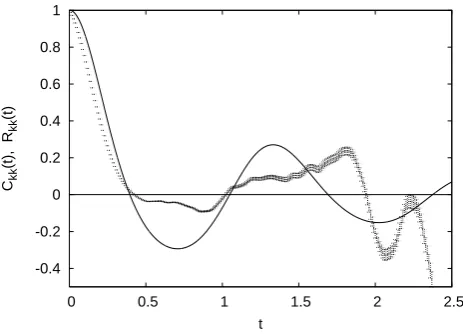
Fig. 2. Lorenz-96 model: autocorrelationCkk(t)(full line) and self-responseRkk(t), with statistical error bars,
of the slow variablexk(t)(k= 3).
24
Fig. 2. Lorenz-96 model: autocorrelationCkk(t )(full line) and
self-responseRkk(t ), with statistical error bars, of the slow variable
xk(t )(k=3).
hηi(t )ηj(t0)i=δijδ(t−t0). Although there exist general mathematical results (Givon et al., 2004) on the possibility to derive Eq. (9) from Eqs. (7) and (8), in practice one has to invoke (rather crude) approximations based on physical intuition to determine the shape of feff andbσ (Mazzino et
al., 2005). At this regard, see also the contribution to the volume by Imkeller and von Storch (2001) about stochastic climate models. For a more rigorous approach in some climate problems see Majda et al. (1999, 2001) and Majda and Franzke (2006).
In the following, we analyse and discuss two models which, in spite of their apparent simplicity, contain the ba-sic features, and the same difficulties, of the general
multi--0.4 -0.2 0 0.2 0.4 0.6 0.8 1
0 0.5 1 1.5 2 2.5 Ckk
(t), C
zk
(t)
t
Fig. 3. Lorenz-96 model: autocorrelationCzk(t)(dashed line) of the cumulative variablezk(t)compared to
the autocorrelationCkk(t)ofxk(t)(full line).
25
Fig. 3. Lorenz-96 model: autocorrelationCzk(t )(dashed line)
of the cumulative variablezk(t )compared to the autocorrelation
Ckk(t )ofxk(t )(full line).
scale approach: the Lorenz-96 model (Lorenz, 1996) and a double-well potential with deterministic chaotic forcing. 3.1 The Lorenz-96 model
First, let us consider the Lorenz-96 system (Lorenz, 1996), introduced as a simplified model for the atmospheric circula-tion. Define the set{xk(t )}, fork=1, ..., Nk, and{yk,j(t )}, for j=1, ..., Nj, as the slow large-scale variables and the fast small-scale variables, respectively (being Nk=36 and
Nj=10). Roughly speaking, the{xk}’s represent the synop-tic scales while the{yk,j}’s represent the convective scales. The forced dissipative equations of motion are:
dxk
dt = −xk−1(xk−2−xk+1)−νxk+F +c1
Nj X
j=1
yk,j (10)
dyk,j
dt = −cbyk,j+1(yk,j+2−yk,j−1)−cνyk,j+c1xk (11)
where:F=10 is the forcing term,ν=1 is the linear damping coefficient,c=10 is the ratio between slow and fast charac-teristic times,b=10 is the relative amplitude between large scale and small scale variables, andc1=c/b=1 is the
cou-pling constant that determines the amount of reciprocal feed-back.
Let us consider, first, the response properties of fast and slow variables, see Figs. 1 and 2.
In Fig. 1, the autocorrelation Cjj(t ) and self-response
Rjj(t )refer to the fast variableyk,j(t ), with fixedkandj. It is well evident how, even in absence of a precise agree-ment between autocorrelations and self-response functions (due to the non Gaussian character of the system), one has that the correlation of the slow (fast) variables have at least a
10 15 20 25 30 35 40 45 50 xk
(t)
t
Fig. 4. Lorenz-96 model: time signal sample of the slow variablexk(t)(k= 3) for the deterministic model
(full line) and for the stochastic model (dashed line). For clarity, the two signals have been shifted from each
other along the vertical axis.
26
Fig. 4. Lorenz-96 model: time signal sample of the slow
vari-ablexk(t )(k=3) for the deterministic model (full line) and for the
stochastic model (dashed line). For clarity, the two signals have been shifted from each other along the vertical axis.
qualitative resemblance with the response of the slow (fast) variables themselves.
The structure of the Lorenz-96 model includes a rather nat-ural set of quantities that suggests how to parameterize the effects of the fast variables on the slow variables, for each
k. Let us indicate with zk=P Nj
j=1yk,j the term containing
all theNjfast terms in the equations for theNkslow modes. In the following, we will see that, replacing the determinis-tic terms{zk}’s in the equations for the{xk}’s with suitable stochastic processes, one obtains an effective model able to reproduce the main statistical features of the slow compo-nents of the original system.
It’s worth-noting, from Fig. 3, thatCkk(t )andCzk(t ), the
autocorrelation of the cumulative variable zk(t ), are rather close to each other. This suggests thatzk(t )must be corre-lated toxk(t ), in other words, the cumulative effects of the
Nj fast variablesyk,j(t )onxk(t )are equivalent to an effec-tive slow term, proportional toxk(t ).
We look, therefore, for a conditional white noise parame-terization that takes into account this important information given by the structure of the Lorenz-96 model equations. Let us write the effective equations for the slow modes as
dxk
dt = −xk−1(xk−2−xk+1)−(ν+ν
0
)xk+(F+F0)+c2·ηk (12)
whereηkare uncorrelated and normalized white-noise terms. Some authors, Majda et al. (1999, 2001) and Majda and Franzke (2006), using multiscale methods, have obtained ef-fective Langevin equations for the slow variables of systems having the same structure as the Lorenz-96 model.
Basically we can say that, in the effective model for the slow variables, one parameterizes the effects of the fast variables with a suitable renormalization of the forcing,
F→F+F0, of the viscosity,ν→ν+ν0, and the addition of a
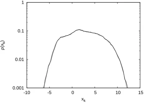
0.001 0.01 0.1 1
-10 -5 0 5 10 15
ρ
(zk
)
zk
Fig. 5. Lorenz-96 model: PDFs of the cumulative variablezk(k= 3), see definition in the text for the two
cases, for the deterministic model (full line) and the stochastic model (dashed line).
27
Fig. 5. Lorenz-96 model: PDFs of the cumulative variablezk
(k=3), see definition in the text for the two cases, for the
deter-ministic model (full line) and the stochastic model (dashed line).
0.001 0.01 0.1 1
-10 -5 0 5 10 15
ρ
(xk
)
xk
Fig. 6. Lorenz-96 model: PDFs of the slow variablexk(k= 3) for the deterministic model (full line) and the
stochastic model (dashed line).
28
Fig. 6. Lorenz-96 model: PDFs of the slow variablexk(k=3) for
the deterministic model (full line) and the stochastic model (dashed line).
random term. In other words, we replace thezk=P Nj
j=1yk,j terms in Eq. (10) with stochastic processeszek depending on the slow variablesxk:
dxk
dt = −xk−1(xk−2−xk+1)−νxk+F +ce1zek (13)
where
e zk=
1
e c1
−ν0xk+F0+c2ηk (14) withce1is a new coupling constant. We notice that Eq. (13)
has the same form of Eq. (10). With a proper choice ofν0,
F0 andc2 in Eq. (12),ν0=−0.3, F0=0.25,c2=0.3, which
impliesce1=0.25 in Eq. (13), one can reproduce the statistics
686 G. Lacorata and A. Vulpiani: FRR with fast and slow dynamics
-0.4 -0.2 0 0.2 0.4 0.6 0.8 1
0 0.5 1 1.5 2 2.5 Ckk
(t), R
kk
(t)
t
Fig. 7. Lorenz-96 model: autocorrelationCkk(t)(full line) and self-responseRkk(t), with statistical error bars,
of the slow variablexk(t)for the stochastic model.
29
Fig. 7. Lorenz-96 model: autocorrelationCkk(t )(full line) and
self-responseRkk(t ), with statistical error bars, of the slow variable
xk(t )for the stochastic model.
ofxkandzk to a very good extent, see at this regard Figs. 4, 5 and 6. Of course the above described parameterization of the fast variables is inspired to the general “philosophy” of the Large-Eddy Simulation of turbulent geophysical flows at high Reynolds numbers (Moeng, 1984; Moeng and Sullivan, 1994; Sullivan et al., 1994).
The FR properties of the stochastic Lorenz-96 slow vari-ables are reported in Fig. 7.
Let us come back to the response problem. Of course the mean response of a slow variable to a perturbation on a fast variable is zero. However, this does not mean that the effect of the fast variables on the slow dynamics is not statistically relevant. Let us introduce the quadratic response of xk(t ) with respect to an infinitesimal perturbation onyk,j(0), for fixedkandj:
Rkj(q)(t )=
h δxk(t )2
i1/2
δyk,j(0)
(15) Considered that in all simulations the initial impulsive per-turbations on the yk,j is kept constant, δyk,j(0)=1, with
1hyk,j2 i1/2, it is convenient to take the average of Eq. (15) over allj’s, at a fixedk, and introduce the quantity:
Rsf(q)(t )= 1
Nj Nj X
j=1
Rkj(q)(t ) (16)
where withsandf we label the slow and fast variables, re-spectively. In the case of the Lorenz-96 system, all theyk,j variables, at fixed k, are statistically equivalent, and have identical coupling withxk, so thatRsf(q)(t )/1coincides with
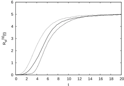
Rkj(q)(t ). We report in Fig. 8 the behavior ofRsf(q)(t ), for both Eqs. (10) and (13). As regards to the stochastic model, the analogous of Eq. (16) is defined as follows. One studies the
0 1 2 3 4 5 6
0 2 4 6 8 10 12 14 16 18 20 Rsf
(q)
(t)
t
Fig. 8. Lorenz-96 model: quadratic cross-response functionR(sfq)(t)for the deterministic model (full line), for
the stochastic model when the slow variables evolve with the same noise realization for all components except
one (dashed line), and when the slow variables evolve with a different noise realization for every component
(dotted line).
30
Fig. 8. Lorenz-96 model: quadratic cross-response function
Rsf(q)(t )for the deterministic model (full line), for the stochastic
model when the slow variables evolve with the same noise realiza-tion for all components except one (dashed line), and when the slow variables evolve with a different noise realization for every compo-nent (dotted line).
evolution ofδxk(t )as difference of two trajectories obtained with two different realizations of the{ηk}’s. It is worth stress-ing that the behavior ofδxk(t )under two noise realizations can be very different from the behavior ofδxk(t )under the same noise realization (see Appendix C). This aspect will be considered again in the next section.
3.2 A simplified model
In order to grasp the essence of systems with fast and slow variables, we discuss now a toy climate model in which the “climatic” variable fluctuates between two states. Consider a four dimensional state vectorq=(q0, q1, q2, q3)whose
evo-lution is given by:
dq0
dt =2
√
H q0−q03+cq1 (17)
dq1
dt =
1
e
[−σL(q1−q2)] (18)
dq2
dt =
1
e
[−q1q3+rLq1−q2] (19) dq3
dt =
1
e
[q1q2−bLq3] (20)
This four equation system will be named the deterministic DW model. The subsystem formed by Eqs. (18), (19) and (20) is nothing but the well-known Lorenz-63 model (Lorenz 1963), in which the constante has the function of rescal-ing the characteristic time. In absence of couplrescal-ing (c=0) be-tweenq0andq1, the unforced motion equation holds for the
-4 -3 -2 -1 0 1 2 3 4
0 50 100 150 200 250 300 350 400 450 500 q0
(t)
t
Fig. 9. DW model withe= 1: time signal sample of the slow variableq0(t). The ratio between fast and slow
characteristic times is∼0.1(see text).
31
Fig. 9. DW model withe=1: time signal sample of the slow
vari-ableq0(t ). The ratio between fast and slow characteristic times is
∼0.1 (see text).
slow variablex=q0: dx
dt = −
∂V
∂x =2
√
H x−x3
with
V (x)=H−
√
H x2+1 4x
4 (21)
The system (21) has one unstable steady state inx0=0
cor-responding to the top of the hill of heightH, and two stable steady states inx1/2=±(4H )1/4, i.e. the bottom of the
val-leys. The presence of the coupling (c6=0) between slow and fast variables can induce transitions between the two valleys. The parameters in Eqs. (17), (18), (19), and (20) are fixed to the following values: σL=10, rL=28, bL=8/3, i.e. the classical set-up corresponding to the chaotic regime for the Lorenz-63 system; H=4, the height of the barrier; c=0.5, the coupling constant that rules the transition time scale of
q0(t )between the two valleys; by settinge=1, the ratio
be-tween fast and slow characteristic times, see Eqs. (7) and (8), isO(10−1).
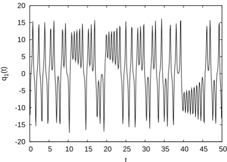
Since the time scale of theq0(t )well-to-well transitions
may be considerably longer, depending on 1/c, than the char-acteristic time ofq1(t ), of orderO(1), we refer toq0as the
slow variable, or the low-frequency observable, and toq1as
the fast variable, or the high-frequency forcing, of the deter-ministic DW model. It can be easily shown that, forc=0, small perturbations 1q0 around the two potential minima
at±(4H )1/4 relax exponentially to zero with characteristic time 1/4
√
H. For sufficiently large values ofc, the climatic variableq0(t )jumps aperiodically back and forth between
the two valleys, driven by the chaotic signalq1(t ), see Figs. 9
and 10.
The main statistical quantities investigated to analyse the DW model are the following:
-20 -15 -10 -5 0 5 10 15 20
0 5 10 15 20 25 30 35 40 45 50 q1
(t)
t
Fig. 10. DW model withe= 1: time signal sample of the fast variableq1(t).
32
Fig. 10. DW model withe=1: time signal sample of the fast
vari-ableq1(t ).
a) the probability density function of the slow variableq0;
b) the probability density function of the well-to-well tran-sition timete,ρ(te);
c) the slow and fast auto-correlation functions (ACF)
Cii(t )=hqi(t )qi(0)i/hqi2i, withi=0,1;
d) the slow and fast self-response functions (ARF)
Rii(t )=δqi(t )/δqi(0), withi=0,1;
e) the quadratic cross-response function of the slow vari-ableq0(t )with respect to the fast variableq1(0).
Of courseR01(t ), i.e. the mean response ofq0(t )to a
per-turbation onq1(0), is zero for trivial symmetry arguments.
On the other hand, the quadratic response:
R01(q)(t )=
h δq0(t )2
i1/2
δq1(0)
(22) can give relevant physical information. Even in this case, since in all simulations the initial perturbation on q1(0)is
kept constant,δq1(0)=1hq12i1/2, it is convenient to define
as mean quadratic response of the slow variable (s) with re-spect to the fast variable (f) the quantityRsf(q)(t )=1·R(q)01(t ). The long-time saturation level ofRsf(q)(t )is of the order of the distance between the two climatic states.
With the current set-up, slow and fast variable have char-acteristic times which differ by an order of magnitude from each other, while the statistics ofq0 is strongly non
Gaus-sian. Because of the skew structure of the system, i.e. the fast dynamics drives the slow dynamics but without counter-feedback, one expects that, at the least in the limit of large time scale separation, the joint PDF can be factorized, with an asymptotic PDF forq0of the formρ0=K·e−Veff(q0), where Kis a normalization constant.
688 G. Lacorata and A. Vulpiani: FRR with fast and slow dynamics
-0.2 0 0.2 0.4 0.6 0.8 1
0 0.2 0.4 0.6 0.8 1 1.2 1.4 1.6 1.8 2 R11
(t), C
11
(t)
t
Fig. 11. DW model withe= 1: autocorrelationC11(t)(full line) and self-responseR11(t), with statistical
error bars, for the fast variableq1.
33
Fig. 11. DW model withe=1: autocorrelationC11(t )(full line)
and self-responseR11(t ), with statistical error bars, for the fast
vari-ableq1.
-0.2 0 0.2 0.4 0.6 0.8 1
0 2 4 6 8 10 12 14 16 18 20 R00
(t), C
00
(t)
t
Fig. 12. DW model withe= 1: AutocorrelationC00(t)(full line) and self-responseR00(t), with statistical
error bars, for the slow variableq0.
34
Fig. 12. DW model withe=1: AutocorrelationC00(t )(full line)
and self-responseR00(t ), with statistical error bars, for the slow
variableq0.
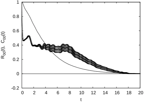
The FR properties of the deterministic DW model, for the fast and slow variables, are shown in Figs. 11 and 12, respec-tively.
The slow self-responseR00(t )initially decreases
exponen-tially with characteristic time 1/4 √
H (H=4), i.e. the same behavior of the relaxation of a small perturbation near the bottom of a valley for c=0. Then, R00(t )relaxes to zero
much more slowly. It is natural to assume that this is due to the long-time jumps between the valleys. It is well evident thatR00behaves rather differently fromC00, whileR11 and C11 have, at least, the same qualitative shape. On the other
hand, the autocorrelation (self-response) time scales of the two variables differ from each other of a factor∼10, compat-ibly with the fact that the ratio between fast and slow charac-teristic times is∼0.1, for the current set-up (e=1).
-0.2 0 0.2 0.4 0.6 0.8 1
0 5 10 15 20 R00
(t), C
00
(t), C(t)
t
Fig. 13. DW model withe= 0.01, implying∼10
−3
: autocorrelationC00(t)(dashed line), self-response
R00(t), with statistical error bars, and the correlation functionC(t)predicted by the FRR (full line) which is actually undistinguishable from the response.
35
Fig. 13. DW model withe=0.01, implying∼10
−3:
autocorrela-tionC00(t )(dashed line), self-responseR00(t ), with statistical error
bars, and the correlation functionC(t )predicted by the FRR (full
line) which is actually undistinguishable from the response.
Since the statistics is far from being Gaussian, the “cor-rect” correlation function which satisfies the FR theorem, for the slow variable, has the form:
C(t )= −
q0(t )
∂ρ(q0, q1, q2, q3) ∂q0
t=0
(23) whereρ(q0, q1, q2, q3)is the (unknown) joint PDF of the
state variable of the system at a fixed. In the limit of large time separation, i.e. fore→0, one expects that the asymptotic PDFρ0(q0, q1, q2, q3)is factorized:
ρ0(q0, q1, q2, q3)=Ke−Veff(q0)ρL(q1, q2, q3) (24)
whereK is a normalization constant, andρLis the PDF of the Lorenz-63 state variable. Under this condition, the right correlation function predicted by the FRR has a relatively simple form:
C(t )=
q0(t )
∂Veff(q0) ∂q0
t=0
(25) whereVeffindicates the effective potential. For∼10−1
(cor-responding toe=1) we have checked numerically that the joint PDF is not yet factorized, while for a very small ra-tio between the characteristic times,∼10−3(corresponding toe=10−2), the form (24) holds and, takingVeff ∝ V, we
obtain a very good agreement betweenR00(t )andC(t ), see
Fig. 13.
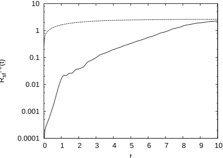
The cross-response properties of the DW model, measured by the quantity R(q)sf (t ), are reported in Fig. 18. We will consider again later this issue when discussing the stochas-tic modeling. While the mean (slow-to-fast) cross-response is null (not shown), its fluctuations grow with time. This means that an initial uncertainty on the fast variables has con-sequences for the predictability of the slow variable, since it
0.0001 0.001 0.01 0.1
0 10 20 30 40 50 60 70
ρ
(te
)
te
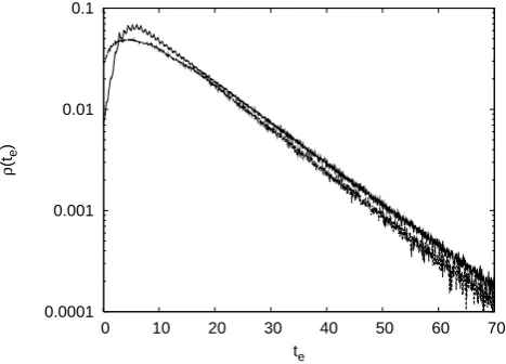
Fig. 14. Comparison of the PDFs of the transition timetebetween the two climatic states for the DW model
(full line) and the WNDW model (dashed line), fore= 1(∼0.1).
36
Fig. 14. Comparison of the PDFs of the transition timetebetween
the two climatic states for the DW model (full line) and the WNDW
model (dashed line), fore=1 (∼0.1).
induces a mean separation growth between two initially close “climatic” states of theq0variable. At small times,Rsf(q)(t )
grows exponentially in time, i.e. it is driven by the chaotic character of the fast variable while, at very long times, the well-to-well aperiodic jumps play the dominant role and the growth speed eventually decreases to zero until saturation sets in.
Let us now consider a stochastic model for the slow vari-ableq0(t ), obtained by replacing the fast variableq1, in the
equation for q0, with a white noise. One has a Langevin
equation of the kind:
dq0 dt (t )=2
√
H q0(t )−q03+σ·ξ(t ) (26)
where ξ(t ) is a Gaussian process with hξ(t )i=0 and hξ(t )ξ(t0)i=δ(t−t0). We call Eq. (26) the WNDW model. The valueσ=19.75 is determined by requiring that the PDFs of the well-to-well transition times have the same asymptotic behavior (i.e. exponential tail with the same exponent), see Fig. 14.
Let us notice that, in this case, because of the skew struc-ture of the original system, the stochastic modeling is (rel-atively) simple and, differently from the generic case, the noise is additive. The time signalq0(t )obtained from the
WNWD model is reported in Fig. 15. One observes strong similarities in the long-time transition statistics with respect to the deterministic model, even though the PDFs of the slow variable are quite different from one another, see Fig. 16.
The FR properties of the WNDW model are reported in Fig. 17. The slow variable is distributed according to ∼e−V (q0)/K, withK=σ2/2, and the FR theorem prediction is verified, i.e. one has a good agreement betweenR00(t )and
the correlation functionC(t ).
-4 -3 -2 -1 0 1 2 3 4
0 50 100 150 200 250 300 350 400 450 500 q0
(t)
t
Fig. 15. WNDW model: time signal sample of the slow variableq0(t).
37
Fig. 15. WNDW model: time signal sample of the slow variable
q0(t ).
0 0.1 0.2 0.3 0.4 0.5 0.6 0.7
-3 -2 -1 0 1 2 3
ρ
(q
0
)
q0
Fig. 16. PDFs of the slow variableq0for the DW model withe= 1, i.e.∼0.1(full line), the WNDW model
(dashed line) and the DW model withe= 10 −2
, i.e.∼10−3
(dotted line). In the limit→0, the PDFs of the deterministic model and of the stochastic model collapse.
38
Fig. 16. PDFs of the slow variableq0for the DW model withe=1,
i.e.∼0.1 (full line), the WNDW model (dashed line) and the DW
model withe=10−2, i.e.∼10−3(dotted line). In the limit→0,
the PDFs of the deterministic model and of the stochastic model collapse.
We redefine, as already seen when discussing the stochas-tic model approximating the Lorenz-96 system, the quadrastochas-tic cross-response function R(q)sf (t ) as the root mean square growth of the errorδq0(t )induced by two different noise
re-alizations.
In Fig. 18, the behavior ofR(q)sf (t )for the deterministic DW system and its stochastic model is reported. The WNDW model is not able to reproduce the two-time behavior of the deterministic model, mainly due to the impossibility to con-trol the amplitude of the initial perturbation. Because of that, the error on the climatic state of the system saturate very quickly, as soon as the trajectory starts jumping between the wells.
690 G. Lacorata and A. Vulpiani: FRR with fast and slow dynamics
-0.2 0 0.2 0.4 0.6 0.8 1
0 2 4 6 8 10 12 14 16 18 20 R00
(t), C
00
(t), C(t)
t
Fig. 17. WNDW model: autocorrelationC00(t)(dashed line), self-responseR00(t), with statistical error bars,
and the correlation functionC(t)predicted by the FRR (full line).
39
Fig. 17. WNDW model: autocorrelationC00(t )(dashed line),
self-responseR00(t ), with statistical error bars, and the correlation
func-tionC(t )predicted by the FRR (full line).
4 Discussion and conclusive remarks
In this paper we have presented a detailed investigation of the Fluctuation-Response properties of chaotic systems with fast and slow dynamics. The numerical study has been performed on two models, namely the 360-variable Lorenz-96 system, with reciprocal feedback between fast and slow variables, and a simplified low dimensional system, both of which are able to capture the main features, and related difficulties, typ-ical of the multiscale systems. The first point we wish to emphasize is how, even in non Hamiltonian systems, a gen-eralized Fluctuation-Response Relation (FRR) holds. This allows for a link between the average relaxation of pertur-bations and the statistical properties (correlation functions) of the unperturbed system. Although one has non Gaus-sian statistics, the correlation functions of the slow (fast) variables have at least a qualitative resemblance with the re-sponse functions to perturbations on the slow (fast) degrees of freedom. The average response function of a slow variable to perturbations of the fast degrees of freedom is zero, never-theless the impact of the fast dynamics on the slowly varying components cannot be neglected. This fact is clearly high-lighted by the behavior of a suitable quadratic response func-tion. Such a phenomenon, which can be regarded as a sort of sensitivity of the slow variables to variations of the fast components, has an important consequence for the modeling of the slow dynamics in terms of a Langevin equation. Even an optimal model (i.e. able to mimic autocorrelation and self-response of the slow variable), beyond a certain intrinsic time interval, can give just statistical predictions, in the sense that, at most, one can hope to have an agreement among the statis-tical features of system and model. In stochastic dynamical systems, one has to deal with a similar behavior: the relevant “complexity” of the systems is obtained by considering the
0.0001 0.001 0.01 0.1 1 10
0 1 2 3 4 5 6 7 8 9 10 Rsf
(q)
(t)
t
Fig. 18. Quadratic cross-response functionR(sfq)(t)for the DW model (full line) and the WNDW model (dashed
line). The growth rates ofR(sfq)(t)for the DW model are compatible with the two characteristic times of the system, while for the WNDW modelR(sfq)(t)quickly saturates in a very short time.
40
Fig. 18. Quadratic cross-response functionRsf(q)(t )for the DW model (full line) and the WNDW model (dashed line). The growth
rates ofRsf(q)(t )for the DW model are compatible with the two
char-acteristic times of the system, while for the WNDW modelRsf(q)(t )
quickly saturates in a very short time.
divergence of nearby trajectories evolving under two differ-ent noise realizations. Therefore a good model for the slow dynamics (e.g. a Langevin equation) must show a sensitivity to the noise.
Appendix A
Generalized FRR
In this Appendix we give a derivation, under general rather hypothesis, of a generalized FRR. Consider a dynamical sys-tem x(0)→x(t )=Utx(0) with states x belonging to a N -dimensional vector space. For the sake of generality, we will consider the case in which the time evolution can also be not completely deterministic (e.g. stochastic differential equations). We assume the existence of an invariant proba-bility distributionρ(x), for which some “absolute continuity” type conditions are required (see later), and the mixing char-acter of the system (from which its ergodicity follows). Note that no assumption is made onN.
Our aim is to express the average response of a generic observableAto a perturbation, in terms of suitable correla-tion funccorrela-tions, computed according to the invariant measure of the unperturbed system. At the first step we study the behavior of one component of x, sayxi, when the system, described by ρ(x), is subjected to an initial (non-random) perturbation such that x(0)→x(0)+1x0. This instantaneous
kick3modifies the density of the system intoρ0(x), related to
3The study of an “impulsive” perturbation is not a severe
limita-tion, e.g. in the linear regime from the (differential) linear response
the invariant distribution byρ0(x)=ρ(x−1x0). We introduce
the probability of transition from x0 at time 0 to x at time t, W (x0,0→x, t ). For a deterministic system, with
evolu-tion law x(t )=Utx(0), the probability of transition reduces to
W (x0,0→x, t )=δ(x−Utx0), whereδ(·)is the Dirac’s delta.
Then we can write an expression for the mean value of the variablexi, computed with the density of the perturbed sys-tem:
D xi(t )
E0
=
Z Z
xiρ0(x0)W (x0,0→x, t ) dxdx0. (A1)
The mean value ofxi during the unperturbed evolution can be written in a similar way:
D xi(t )
E
=
Z Z
xiρ(x0)W (x0,0→x, t ) dxdx0. (A2)
Therefore, definingδxi=hxii0−hxii, we have:
δxi(t )=
Z Z
xi F (x0, 1x0) ρ(x0)W (x0,0→x, t ) dxdx0
=Dxi(t ) F (x0, 1x0) E
(A3) where
F (x0, 1x0)= ρ(x
0−1x0)−ρ(x0) ρ(x0)
. (A4)
Let us note here that the mixing property of the system is re-quired so that the decay to zero of the time-correlation func-tions assures the switching off of the deviafunc-tions from equi-librium.
For an infinitesimal perturbationδx(0)=(δx1(0)· · ·δxN
(0)), ifρ(x)is non-vanishing and differentiable, the function in Eq. (A4) can be expanded to first order and one obtains:
δxi(t )= −
X
j
* xi(t )
∂lnρ(x) ∂xj
t=0 +
δxj(0)
≡X
j
Rij(t )δxj(0) (A5)
which defines the linear response
Rij(t )= −
* xi(t )
∂lnρ(x) ∂xj
t=0 +
(A6)
of the variablexi with respect to a perturbation ofxj. One can easily repeat the computation for a generic observable
A(x):
δA (t )= −X j
*
A(x(t )) ∂lnρ(x) ∂xj
t=0 +
δxj(0) . (A7)
For Langevin equations, the differentiability ofρ(X)is well established. On the contrary, one could argue that in a
one understands the effect of a generic perturbation.
chaotic deterministic dissipative system the above machin-ery cannot be applied, because the invariant measure is not smooth at all. Typically the invariant measure of a chaotic at-tractor has a multifractal character and its Renyi dimensions
dq are not constant (Paladin and Vulpiani, 1987). In chaotic dissipative systems the invariant measure is singular, how-ever the previous derivation of the FRR is still valid if one considers perturbations along the expanding directions. For a mathematically oriented presentation see Ruelle (1998). A general response function has two contributions, correspond-ing respectively to the expandcorrespond-ing (unstable) and the contract-ing (stable) directions of the dynamics. The first contribution can be associated to some correlation function of the dynam-ics on the attractor (i.e. the unperturbed system). On the con-trary this is not true for the second contribution (from the contracting directions), this part to the response is very dif-ficult to extract numerically (Cessac and Sepulchre, 2007). In chaotic deterministic systems, in order to have a differ-entiable invariant measure, one has to invoke the stochastic regularization (Zeeman, 1990). If such a method is not feasi-ble, one can use the direct approach by Abramov and Majda (2007). For a study of the FRR in chaotic atmospheric sys-tems, see Dymnikov and Gritsoun (2005) and Gritsoun and Branstator (2007).
Let us notice that a small amount of noise, that is always present in a physical system, smoothen theρ(x)and the FRR can be derived. We recall that this “beneficial” noise has the important role of selecting the natural measure, and, in the numerical experiments, it is provided by the round-off errors of the computer. We stress that the assumption on the smoothness of the invariant measure allows to avoid subtle technical difficulties.
Appendix B
A general remark on the decay of correlation functions
Using some general arguments one has that all the (typical) correlation functions at large time delay have to relax to zero with the same characteristic time, related to spectral proper-ties of the operatorL which rules the time evolution of theˆ
P (X, t ):
∂
∂tP (X, t )= ˆLP (X, t ) . (B1)
In the case of ordinary differential equations
dXi/dt=Qi(X) i=1,· · ·, N (B2) the operatorL has the shapeˆ
ˆ
LP (X, t )= −X i
∂ ∂Xi
Qi(X)P (X, t )
. (B3)
692 G. Lacorata and A. Vulpiani: FRR with fast and slow dynamics For Langevin equations i.e. in Eq. (B2)Qi is replaced by
Qi+ηi where{ηi}are Gaussian processes with<ηi(t )>=0 and<ηi(t )ηj(t0)>=23i,jδ(t−t0), one has
ˆ
LP (X, t )= −P
i ∂X∂i
Qi(X)P (X, t )
+P
ab3i,j ∂
2
∂Xi∂XiP (X, t ) .
(B4)
Let us introduce the eigenvalues{αk}and the eigenfunc-tions{ψk}ofL:
ˆ
Lψk=αkψk. (B5)
Of courseψ0=Pinv andα0=0, and typically in mixing
sys-temsRe αk<0 fork=1,2, .... Furthermore assuming that co-efficient{g1, g2, ...}and{h1, h2, ...}exist such that functions g(X)andh(X)are uniquely expanded as
g(X)=X
k=0
gkψk(X) , h(X)=
X
k=0
hkψk(X) , (B6)
so we have
Cg,f(t )=
X
k=1
gkhk< ψk2> e
αkt, (B7)
where Cg,f(t )=<g(X(t ))h(X(t ))>−<g(X)><h(X)>. For “generic” functions g and f, i.e. if they are not or-thogonal to ψ1 so thatg16=0 and h16=0, at large time the
correlationCg,f(t )approaches to zero as
Cg,f(t )∼e−t /τc , τc= 1 |Re α1|
. (B8)
In some cases, e.g. very intermittent systems like the Lorenz model atr'166.07,Re α1=0 so the decay is not
ex-ponentially fast.
Appendix C
Lyapunov exponent in dynamical systems with noise
In systems with noise, the simplest way to introduce the Lyapunov exponent is to treat the random term as a time-dependent term. Basically one considers the separation of two close trajectories with the same realization of noise. Only for sake of simplicity consider a one-dimensional Langevin equation
dx
dt = −
∂V (x)
∂x +σ η , (C1)
whereη(t )is a white noise andV (x)diverges for|x| →∞, like, e.g., the usual double well potentialV=−x2/2+x4/4.
The Lyapunov exponentλσ, associated with the separation rate of two nearby trajectories with the same realization of
η(t ), is defined as
λσ = lim t→∞
1
t ln|z(t )| (C2)
where the evolution of the tangent vector is given by:
dz
dt = −
∂2V (x(t ))
∂x2 z(t ). (C3)
The quantityλσ obtained in the previous way, although well defined, i.e. the Oseledec theorem (Bohr et al., 1998) holds, it is not always a useful characterization of complexity.
Since the system is ergodic with invariant probability dis-tribution P (x)=C1e−V (x)/C2, where C1 is a normalization
constant andC2=σ2/2, one has: λσ =limt→∞1t ln|z(t )|
= −limt→∞1t Rt
0∂ 2
xxV (x(t 0))dt0
= −C1R ∂xx2 V (x)e−V (x)/C2 dx = −C1
C2
R
(∂xV (x))2e−V (x)/C2 dx <0.
(C4)
This has a rather intuitive meaning: the trajectoryx(t )spends most of the time in one of the “valleys” where−∂xx2 V (x)<0 and only short intervals on the “hills” where−∂xx2 V (x)>0, so that the distance between two trajectories evolving with the same noise realization decreases on average. The previ-ous result for the 1-D Langevin equation can easily be gen-eralized to any dimension for gradient systems if the noise is small enough (Loreto et al., 1996).
A negative value ofλσ implies a fully predictable process only if the realization of the noise is known. In the case of two initially close trajectories evolving under two different noise realizations, after a certain timeTσ, the two trajecto-ries can be very distant, because they can be in two different valleys. Forσ→0, due to the Kramers formula (Gardiner, 1990), one hasTσ∼e1V /σ
2
, where1V is the difference be-tween the values ofV on the top of the hill and at the bottom of the valley.
Let us now discuss the main difficulties in defining the no-tion of “complexity” of an evoluno-tion law with a random per-turbation, discussing a simple case. Consider the 1-D map
x(t+1)=f[x(t ), t] +σ w(t ), (C5)
wheretis an integer andw(t )is an uncorrelated random pro-cess, e.g.ware independent random variables uniformly dis-tributed in[−1/2,1/2]. For the largest LEλσ, as defined in (C2), now one has to study the equation
z(t+1)=f0[x(t ), t]z(t ), (C6)
wheref0=df/dx.
Following the approach in (Paladin et al., 1995) letx(t )be the trajectory starting atx(0)andx0(t )be the trajectory start-ing fromx0(0)=x(0)+δx(0). Letδ0≡|δx(0)|and indicate by τ1the minimum time such that|x0(τ1)−x(τ1)|≥1. Then, we
putx0(τ1)=x(τ1)+δx(0)and defineτ2as the time such that
|x0(τ1+τ2)−x(τ1+τ2)|>1for the first time, and so on. In
this way the Lyapunov exponent can be defined as
λ= 1
τ ln
1
δ0
(C7)
beingτ=P
τi/N whereN is the number of the intervals in the sequence. If the above procedure is applied by con-sidering the same noise realization for both trajectories,λin Eq. (C2) coincides withλσ (ifλσ>0). Differently, by con-sidering two different realizations of the noise for the two trajectories, we have a new quantity
Kσ = 1
τ ln
1 δ0
, (C8)
which naturally arises in the framework of information the-ory and algorithmic complexity thethe-ory: note thatKσ/ln 2 is the number of bits per unit time one has to specify in order to transmit the sequence with a precisionδ0, The generalization
of the above treatment toN-dimensional maps or to ordinary differential equations is straightforward.
If the fluctuations of the effective Lyapunov expo-nent γ (t ) (in the case of Eq. C5 γ (t ) is nothing but ln|f0(x(t ))|) are very small (i.e. weak intermittency) one has
Kσ=λ+O(σ/1).
The interesting situation happens for strong intermittency when there are alternations of positive and negativeγduring long time intervals: this induces a dramatic change for the value ofKσ. Numerical results on intermittent maps (Pal-adin et al., 1995) show that the same system can be regarded either as regular (i.e.λσ<0), when the same noise realiza-tion is considered for two nearby trajectories, or as chaotic (i.e.Kσ>0), when two different noise realizations are con-sidered. We can say that a negativeλσ for some value of
σ in not an indication that “noise induces order”; a correct conclusion is that noise can induce synchronization.
Acknowledgements. We warmly thank A. Mazzino, S. Musacchio, R. Pasmanter and A. Puglisi for interesting discussions and suggestions, and two anonymous referees for their contructive criticism in reviewing this paper.
Edited by: O. Talagrand
Reviewed by: two anonymous referees
References
Abramov, R. and Majda, A.: New approximations and tests of lin-ear fluctuation-response for chaotic nonlinlin-ear forced-dissipative dynamical systems, J. Nonlinear Sci., accepted, 2007.
Bell, T. L.: Climate sensitivity from fluctuation-dissipation: some simple model tests, J. Atmos. Sci., 37, 1700–1707, 1980. Biferale, L., Daumont, I., Lacorata, G., and Vulpiani, A.:
Fluctuation-response relation in turbulent systems, Phys. Rev. E, 65, 016302, 016302-1–016302-7, 2002.
Boffetta, G., Lacorata, G., Musacchio, S., and Vulpiani, A.: Relax-ation of finite perturbRelax-ations: Beyond the FluctuRelax-ation-Response relation, Chaos, 13, 806–811, 2003.
Bohr, T., Jensen, M. H., Paladin, G., and Vulpiani, A.: Dynami-cal systems approach to turbulence, Cambridge University Press, UK, 1998.
Cane, M.: Understanding and predicting the world’s climate sys-tem, Chaos in geophysical flows, Chaos in geophysical flows, edited by: Boffetta, G., Lacorata, G., Visconti, G., and Vulpiani, A., Otto Eds., Torino, Italy, 2003.
Cessac, B. and Sepulchre, J.-A.: Linear response, susceptibility and resonance in chaotic toy models, Physica D, 225, 13–28, 2007. Cionni, I., Visconti, G., and Sassi, F.: Fluctuation-dissipation
the-orem in a general circulation model, Geophys. Res. Lett., 31, L09206, doi:10.1029/2004GL019739, 2004.
Deker, U. and Haake, F.: Fluctuation-dissipation theorems for clas-sical processes, Phys. Rev. A, 11, 2043–2056, 1975.
Ditlevsen, P. D.: Observation ofα-stable noise induced millennial
climate changes from an ice-core record, Geophys. Res. Lett., 26(10), 1441–1444, 1999.
Dymnikov, V. P.: Potential Predictability of Large-Scale Atmo-spheric Processes, Izvestiya, AtmoAtmo-spheric and Oceanic Physics, 40(5), 513–519, 2004.
Dymnikov, V. P. and Gritsoun, A. S.: Climate model attractors: chaos, quasi-regularity and sensitivity to small perturbations of external forcing, Nonlin. Processes Geophys., 8, 201–209, 2001, http://www.nonlin-processes-geophys.net/8/201/2001/.
Dymnikov, V. P. and Gritsoun, A. S.: Current problems in the math-ematical theory of climate, Izvestiya, Atmospheric and Oceanic Physics, 41, 294–314, 2005.
Falcioni, M., Isola, S., and Vulpiani, A.: Correlation functions and relaxation properties in chaotic dynamics and statistical mechan-ics, Phys. Lett. A, 144, 341–346, 1990.
Fraedrich, K.: Predictability: short and long-term memory of the atmosphere, Chaos in geophysical flows, Chaos in geophysical flows, edited by: Boffetta, G., Lacorata, G., Visconti, G., and Vulpiani, A., Otto Eds., Torino, Italy, 2003.
Frisch, U.: Turbulence, Cambridge University Press, UK, 1995. Gardiner, C. W.: Handbook of stochastic methods for Physics,
Chemistry and the Natural Sciences, Springer-Verlag, Berlin, Germany, 1990.
Givon, D., Kupferman, R., and Stuart, A.: Extracting macroscopic dynamics: model problems and algorithms, Nonlinearity, 17, 55– 127, 2004.
Gritsoun, A. S.: Fluctuation-dissipation theorem on attractors of atmospheric models, Russ. J. Numer. Analysis Math. Modelling, 16, 115–133, 2001.
Gritsoun, A. S. and Branstator, G.: Climate Response Using a Three-Dimensional Operator Based on the Fluctuation Dissipa-tion Theorem, J. Atmos. Sci., 64(7), 2558-2575, 2007.
Gritsoun, A. S., Branstator, G., and Dymnikov, V. P.: Construction of the linear response operator of an atmospheric general circu-lation model to small external forcing, Russ. J. Numer. Analysis Math. Modelling, 17, 399–416, 2002.
Gritsoun, A. S. and Dymnikov, V. P.: Barotropic atmosphere re-sponse to small external action: theory and numerical experi-ments, Izvestiya, Atmospheric and Oceanic Physics, 35, 511– 525, 1999.
Haskins, R., Goody, R., and Chen, L.: Radiance covariance and climate models, J. Climate, 12, 1409–1422, 1999.
Hohenberg, P. C. and Shraiman, B. I.: Chaotic behavior of an ex-tended system, Physica D, 37, 109–115, 1989.
Imkeller, P. and von Storch, J.-S. (Eds.): Stochastic Climate Mod-els, Birkh¨auser, Basel, Switzerland, 2001.
Kraichnan, R. H.: Classical fluctuation-relaxation theorem, Phys.
694 G. Lacorata and A. Vulpiani: FRR with fast and slow dynamics
Rev., 113, 1181–1182, 1959.
Kraichnan, R. H.: Deviations from fluctuation-relaxation relations, Physica A, 279, 30–36, 2000.
Kraichnan, R. H. and Montgomery, D.: Two-dimensional turbu-lence, Rep. Prog. Phys., 43, 547–619, 1980.
Kubo, R.: The fluctuation-dissipation theorem, Rep. Prog. Phys., 29, 255–284, 1966.
Kubo, R.: Brownian motion and nonequilibrium statistical mechan-ics, Science, 233, 330–334, 1986.
Leith, C. E.: Climate response and fluctuation-dissipation, J. At-mos. Sci., 32, 2022–2026, 1975.
Leith, C. E.: Predictability of climate, Nature, 276, 352–355, 1978. Lorenz, E. N.: Deterministic nonperiodic flow, J. Atmos. Sci., 20,
130–141, 1963.
Lorenz, E. N.: Predictability – a problem partly solved, Proceed-ings, Seminar on Predictability ECMWF, 1, 1–18, 1996. Loreto, V., Paladin, G., and Vulpiani, A.: On the concept of
com-plexity for random dynamical systems, Phys. Rev. E, 53, 2087– 2098, 1996.
Majda, A. J., Abramov, R., and Grote, M.: Information theory and stochastics for multiscale nonlinear systems, CRM monograph series 25, American Mathematical Society, 2005.
Majda, A. J. and Franzke, C.: Low Order Stochastic Mode Reduc-tion for a Prototype Atmospheric GCM, J. Atmos. Sci., 63(2), 457-479, 2006.
Majda, A. J., Timofeyev, I., and Vanden-Eijnden, E.: Models for stochastic climate prediction, Proc. Natl. Acad. Sci. USA, 96, 14 687–14 691, 1999.
Majda, A. J., Timofeyev, I., and Vanden-Eijnden, E.: A mathe-matical framework for stochastic climate models, Commun. Pure Appl. Math., 54, 891–974, 2001.
Majda, A. J. and Wang, X.: Nonlinear Dynamics and Statistical Theories for Basic Geophysical Flows, Cambridge University Press, UK, 2006.
Marwan, N., Trauth, M., Vuille, M., and Kurths, J.: Comparing modern and Pleistocene ENSO-like influences in NW Argentina using nonlinear time series analysis methods, Clim. Dynam., 21, 317–326, 2003.
Matsumoto, K. and Tsuda, I.: Noise-induced order, J. Stat. Phys., 31, 87–106, 1983.
Mazzino, A., Musacchio, S., and Vulpiani, A.: Multiple scale analy-sis and renormalization for preasymptotic scalar transport, Phys. Rev. E, 71, 011113, 1–11, 2005.
McComb, W. D. and Kiyani, K.: Eulerian spectral closures for isotropic turbulence using a time-ordered fluctuation-dissipation relation, Phys. Rev. E, 72, 016309, 016309-1–016309-12, 2005. Moeng, C.-H.: A Large-Eddy Simulation model for the study of planetary boundary layer turbulence, J. Atmos. Sci., 41, 2052– 2062, 1984.
Moeng, C.-H. and Sullivan, P. P.: A comparison of shear and buoy-ancy driven planetary boundary layer flows, J. Atmos. Sci., 51, 999–1021, 1994.
North, G. R., Bell, R. E., and Hardin, J. W.: Fluctuation dissipation in a general circulation model, Clim. Dynam., 8, 259–264, 1993. Paladin, G., Serva, M., and Vulpiani, A.: Complexity in dynamical
systems with noise, Phys. Rev. Lett., 74, 66–69, 1995.
Paladin, G. and Vulpiani, A.: Anomalous scaling laws in multifrac-tal objects, Phys. Rep., 156, 147–225, 1987.
Pasmanter, R. A.: On long-lived vortices in 2-D viscous flows, most probable states of inviscid 2-D flows and a soliton equa-tion, Phys. Fluids, 6, 1236–1241, 1994.
Pikovsky, A., Rosenblum, M., and Kurths, J.: Synchronization: a universal concept in nonlinear sciences, Cambridge University Press, UK, 2003.
Rose, R. H. and Sulem, P. L.: Fully developed turbulence and sta-tistical mechanics, J. Phys., 39, 441–484, 1978.
Ruelle, D.: General linear response formula in statistical mechan-ics, and the fluctuation-dissipation theorem far from equilibrium, Phys. Lett. A, 245, 220–224, 1998.
Sullivan, P. P., McWilliams, J.-C., and Moeng, C.-H.: A subgrid-scale model for large-eddy simulation of planetary boundary layer flows, Bound. Layer Meteorol., 71, 247–276, 1994. Zeeman, E. C.: Stability of dynamical systems, Nonlinearity, 1,
115–135, 1988.