A Semi-Supervised Machine Learning Approach Using K-Means Algorithm to Prevent Burst Header Packet Flooding Attack in Optical Burst Switching Network

Baghdad Science Journal

Vol.16(3) Supplement 2019

A Semi-Supervised Machine Learning Approach Using K-Means Algorithm to

Prevent Burst Header Packet Flooding Attack in Optical Burst Switching

Network

Muhammad Kamrul Hossain Patwary

Md. Mokammel Haque

Received 3/1/2019, Accepted 20/5/2019, Published 23/9/2019

This work is licensed under a Creative Commons Attribution 4.0 International License.

Abstract:

Optical burst switching (OBS) network is a new generation optical communication technology. In an OBS network, an edge node first sends a control packet, called burst header packet (BHP) which reserves the necessary resources for the upcoming data burst (DB). Once the reservation is complete, the DB starts travelling to its destination through the reserved path. A notable attack on OBS network is BHP flooding attack where an edge node sends BHPs to reserve resources, but never actually sends the associated DB. As a result the reserved resources are wasted and when this happen in sufficiently large scale, a denial of service (DoS) may take place. In this study, we propose a semi-supervised machine learning approach using k-means algorithm, to detect malicious nodes in an OBS network. The proposed semi-supervised model was trained and validated with small amount data from a selected dataset. Experiments show that the model can classify the nodes into either behaving or not-behaving classes with 90% accuracy when trained with just 20% of data. When the nodes are classified into behaving, not-behaving and potentially not-behaving classes, the model shows 65.15% and 71.84% accuracy if trained with 20% and 30% of data respectively. Comparison with some notable works revealed that the proposed model outperforms them in many respects.

Key words: Burst Header Packet Flooding Attack, K-Means Algorithm, Machine Learning, Optical Burst Switching Network, Semi-supervised Learning.

Introduction:

This Optical network (ON) is an effective data communication network that uses light pulses to send and receive data. Optical burst switching (OBS) is a kind of optical network that employs a tradeoff concerning optical circuit switching and optical packet switching (1). The principle of OBS network is simple yet it yields a powerful communication system. After receiving user datagram packets (UDP), the OBS network assembles them in an edge node (ingress node). This is called data burst (DB). At the same time another packet is generated which is called burst header packet (BHP). A BHP holds information about the DB and the destination of the DB. Once the DBs are assembled, the BHP is transmitted form the edge node to reserve the resources of the core nodes needed for the DB to travel to its destination. After a specified interval of sending BHP, the DB is transmitted and it follows the path reserved by the BHP.

Department of Computer Science and Engineering, Chittagong University of Engineering and Technology, Chittagong-4349, Bangladesh

*

Corresponding Author:

[email protected]

DB. In (7) authors designed and implemented an algorithm to classify the ingress nodes of an OBS network into three classes, i.e. Trusted, Blocked, and Suspicious. Based on the node’s behavior and the amount of unutilized reserved resources, the classification was performed. According to the authors, the model can be integrated in the OBS core switch which can enable it to classify the nodes.

The methods described above make heavy use of expert’s opinion to assign labels to the behavior and collected data, i.e. marking whether a behavior is good or bad. Getting expert’s hand-assigned data is not always feasible. In this respect, machine learning architecture can provide a great support in classification of OBS network traffic. Machine learning (ML) has been used profusely in a variety of application areas, including network traffic filtering and classification. ML tries to construct algorithms and models that can learn to make decisions using hidden correlations discovered from historical data. Automatically detecting a misbehaving node is possible using ML based on data related to the node’s behaviors such as packet drop rate, packet received rate, delay time, amount of bandwidth use etc. Thus, it can offer a promising solution to the BHP flood attacks in OBS network. One major application of ML is classification where a model or classifier is constructed to predict class (categorical) labels. The attribute whose value is to be predicted is called target attribute. A classifier predicts the target attribute’s value after going through a learning process using the recorded set of data. In this study, we shall build a classifier to predict the label of an OBS node based on a learning process using the recorded OBS data.

Existing ML algorithms can be divided into at least three categories: supervised learning (SL), Semi-supervised learning (SSML), and unsupervised learning (USL). SL techniques conduct classification tasks using labeled data, while USL techniques focus on classifying the sample sets into different groups, i.e. clusters, using unlabeled data. SSML (8,9) technique makes use of both labeled and unlabeled data when learning. Generally in SSML, labeled instances are used to learn class models and unlabeled instances are used to improve the learning performance. Though SL algorithms generally outperform USL and SSML algorithms, it is not always easy to find properly labeled training data. Labeling data is time consuming, expensive, and sometimes dangerous, e.g. landmine detection. On the other hand, it is much easier to obtain unlabeled data. SSML can make a good use of a big amount of unlabeled data and a relatively small amount of labeled data. With

help of SSML algorithm and proper data, a good classifier can be constructed to classify the nodes of OBS network. One of the most popular and effective yet simple unsupervised machine learning algorithm is k-means algorithm (10). K-means was used to provide promising solutions to numerous problems in diverse application areas (11,12). In this study, we shall use k-means algorithm in a semi-supervised approach. At first, a small set of unlabeled data will be used to train the k-means model. Then, a similar sized labeled data will be used to validate the model. After that, a large dataset will be used to evaluate the performance of the model. In this way, a model will be constructed which will be able to classify the nodes of OBS network into malicious and non-malicious classes.

Decision tree algorithm was used to extract If-Then rules which were used to classify the ingress nodes of OBS network into either Behaving or Misbehaving nodes. The authors further classified the Misbehaving ingress nodes into four sub-classes, i.e. No Block, Misbehaving-Wait, Misbehaving-Block and Behaving-No Block. First, they built a dataset of 1075 records using network simulation software and expert’s hand-assigned target class labels. Then, the dataset was used to perform the training and testing of decision tree model. Their model showed 93% accuracy in case of two class classification, and 87% accuracy in case of four class classification.

This paper proposes a semi-supervised machine learning approach using k-means algorithm. We believe that this study, to our best knowledge, is among the earliest to propose and implement a semi-supervised ML technique using k-means algorithm to prevent BHP flooding attacks by predicting malicious node in an OBS network

Methodology:

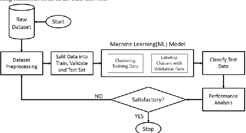
Semi-supervised learning(SSML) deals with small labeled data and relatively big amount of unlabeled data. The small amount of labeled data is used to train a machine learning model which predicts labels for the remaining unlabeled data. In this paper, we used a SSML architecture depicted in Fig. 1. Firstly, we selected a suitable dataset of OBS network node’s data. After preprocessing this raw dataset we split the dataset into three portions, i.e. train, validate and test data. The train data was used for training an unsupervised learning(USL) model. After the training, we validated the clusters obtained from the model. Validation gives labels to the clusters. Using this validated model, the test data was classified and assigned labels. To measure the accuracy of our model’s classification, we compared the actual labels with the predicted labels of test dataset.

Figure 1. The proposed semi-supervised learning architecture to prevent BHP flood attack

Semi-Supervised Model Building through Validation

In order to transform a USL model into a SSML model, a relatively limited amount of labeled data was fed into the model. The labeled data was used to set the labels of the clusters discovered by the USL model. This is called validation. During the splitting of the preprocessed dataset, we take a portion as validate set. This validate set contains a small amount of labeled data. After training a USL model with train data, it predicts the cluster number for each validation set data record. After the prediction, it compares the predicted labels with the actual labels of validate set data. The result of the comparison is used to set the label for each cluster.

Algorithm: SSML model building Method←USL Algorithm

Begin

Retrieve Preprocessed Dataset

Split Dataset into Train, Test, Validate Set ML Model Training with Train Set(method) ML Model Validation with Validate Set(method) Predict cluster number for each validate set record Compute the majority vote for each type of predicted cluster number

Set the label of each cluster based on majority vote ML Model Testing with Test Set(method)

Assess Performance Save Model

End

K-Means Clustering Algorithm:

In this study, we choose k-means algorithm as a USL model. Clustering with k-means algorithm is an unsupervised learning (20). The k-means algorithm clusters the data points into k groups where k is pre-calculated. Initially, k points are chosen at random as cluster centers. Then each data points are assigned to their nearest cluster center based on the Euclidean distance function. After that the centroid or mean of all data points in each cluster is calculated. The process is repeated until the cluster membership of data points stabilizes. The output of the algorithm is the centroids of the k clusters. These centroids can be used to label new data. The goal of k-means algorithm is to minimize the total intra-cluster variance, which is to minimize the sum of the squared error for all the k clusters.

The objective function to minimize is as follows (21):

𝐽(𝑃) = ∑ ∑ ‖𝑧_𝑖− 𝜇_𝑘‖2 𝑧𝑖∈𝑝𝑘

𝐾

𝑘=1

Where, Z = {zi}, i = 1,..,n is set of n d-dimensional points to be clustered

P = {pk}, k = 1,…,K is set of k clusters μk = mean of cluster pk

J(P) = is sum of the squared error over all k clusters

The main steps of k-means algorithm are as follows:

Select an initial partition with k clusters; repeat step (ii) and step (iii) until cluster membership become stable.

Compute a new partition by assigning each data point to its nearest cluster center.

Generate new cluster centers.

Dataset Selection:

The scarcity of reliable data has made the use of machine learning very challenging in detecting malicious attacks in OBS networks. The a trustworthy dataset was collected from popular dataset repository, UCI Machine Learning Repository (22). The dataset has 1075 records with 22 attributes. First 10 rows of the dataset are shown in Table 1. The attributes from A to Z represent all the 22 attributes of the dataset. A brief introduction to the attributes is given below.

Table 1. Dataset(part 1)

A B C D E F G H I J K

3 0.822038 0.190381 1000 0.004815 19.03149 19.03813 0.809619 822.0375 177.9625 1440 9 0.275513 0.729111 100 0.004815 72.88904 72.91114 0.270889 27.55125 72.44875 1440 3 0.923707 0.090383 900 0.000633 9.035834 9.038339 0.909617 831.336 68.664 1440 9 0.368775 0.63771 100 0.000552 63.73784 63.771 0.36229 36.8775 63.1225 1440 3 0.905217 0.10867 800 0.000497 10.86421 10.86698 0.89133 724.1738 75.82625 1440

Table 1. Dataset(part 2)

L M N O P Q R S T U V

90324 73128 17196 1.3E+08 1.05E+08 0.146594 0.780936 0.001838 B 0.023455 NB-No-Block 9048 2451 6598 13029120 3529440 0.517669 0.242451 0.002236 NB 0.460725 Block 81276 73930 7346 1.17E+08 1.06E+08 0.058749 0.886758 0.001751 B 0 No-Block 9048 3278 5770 13029120 4720320 0.522922 0.324522 0.001776 NB 0.439255 Block 72228 64379 7849 1.04E+08 92705760 0.076069 0.869009 0.001767 B 0 No-Block

The letters after the names of the attributes represent the A to Z label of table 1.

Node(A): this is the label of edge node. These nodes send and receive packet.

Utilized bandwidth rate(B): the amount which can be reserved from the allocated bandwidth, i.e. from full bandwidth column.

Packet drop rate(C): packet drop rate for individual node, in percentage

Full bandwidth(D): this is user allocated initial reserved bandwidth for individual node. it is also called reserved bandwidth.

Percentage of lost packet rate(F): packets drop rate, in percentage for individual node.

Percentage of lost byte rate(G): lost byte rate, in percentage for individual node.

Packet received rate(H): total packets received per second for individual node on the basis of reserved bandwidth.

Amount of used bandwidth(I): the amount each individual node could reserve from allocated bandwidth, i.e. from D column.

Lost bandwidth(J): the lost amount of assigned bandwidth.

Packet size byte(K): packets size allocated in byte for individual node to send.

Packet transmitted(L): the amount of total packets transmitted per second for individual node on the basis of allocated bandwidth.

Packet received(M): the amount of total packets received per second for individual node on the basis of reserved bandwidth.

Packet lost(N): the amount of total packets lost per second for individual node on the basis of lost bandwidth.

Transmitted byte(O): total bytes transmitted per second for individual node.

Received byte(P): this is total byte received per second for individual node on the basis of reserved bandwidth.

10-run-avg-drop-rate(Q): this is average of packet drop rate(C) for ten successive iterations in simulation.

10-run-avg-bandwith-use(R): this is the average of bandwidth utilized(B) for ten successive iterations in simulation.

10-run-delay(S): the average of delay time for ten successive iterations in simulation.

Node Status(T): it is the classification of nodes into one of three classes, behaving, potentially not behaving and not behaving.

Flood status(U): the amount of flood per node, in percentage on the basis of packet drop rate.

Class(V): it is the classification of the nodes into one of four classes; NB-No-Block, block, no-block and NB-wait.

The dataset was built from rigorous simulation runs using an OBS network simulator software (23). With the assistance of a domain expert, the authors labeled the dataset’s two categorical attributes, i.e. (B and NB) for the ‘Node Status’ attribute, and (No-Block, NB-No-Block, NB-Wait, and Block) for the ‘Class’ attribute. The category wise label assignments were done based on the intentional false resource utilization rate and the real packet drop rate. Three attributes: avg-bandwith-use, avg-drop-rate, 10-run-delay, each one symbolizes an average value calculated from ten consecutive iterations in the

simulator. This was done to retain the statistical significance and minimize the bias within the node performance results (19). The attributes ‘Node Status(T)’ and ‘Class(V)’ are our target attributes. Discussion about these two attributes is given in later section of this paper.

Implementation Tools:

To perform experimental analysis on our dataset, we used H2O (version 3.18.0.2) (24) which is an open-source data modeling software. Python programming language (25) was chosen for coding, data preprocessing, model building, and performance analysis.

Dataset Preprocessing:

Dataset preprocessing is a vital step in the application of machine learning. It involves transformation of real-world data into an appropriate form so that an ML algorithm can make a good use of it. Real-world data collection process is often loosely controlled which results in incomplete, inconsistent, out of range and missing values. Knowledge discovery with such data is difficult. To resolve such issues data preprocessing is necessary. Data preprocessing includes several step-by-step processes like data cleaning, data transformation, feature selection etc. The preprocessing applied to our OBS network dataset is described below.

Data Cleaning: If an attribute had missing values then those missing fields were filled with the mean of all values of that attribute. The attributes with constant values were removed from dataset because they did not provide any insight in knowledge discovery.

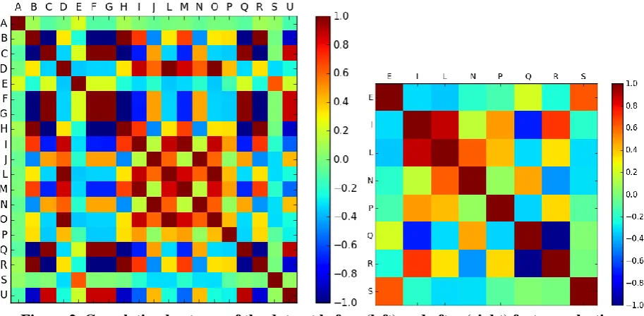
target attribute. After calculating the PCC for every pair of remaining attributes from our OBS network dataset, we found many pairs of positively correlated attributes. Using this PCC values, we generated a correlation matrix in python programming language with the help of ‘pandas’

library. With the help of ‘matplotlib’ library we generated a heatmap to visualize the obtained PCC, as depicted in Fig. 2(left). The bar on the right side of figure shows the relation between color and the value of PCC.

Figure 2. Correlation heatmap of the dataset before (left) and after (right) feature selection

With the help of PCC, 11 attributes were identified as redundant and hence can be removed from the dataset. These 11 attributes are A, B, C, D, F, G, H, J, M, O and U as shown in Table 1. As a result, apart from two target attribute ‘Node Status(T)’ and ‘Class(V)’, 8 attributes are available to be used in training the desired ML model. Those are:

Average delay time per sec (E) Amount of used bandwidth (I) Packet transmitted (L)

Packet lost (N) Received byte (P)

10-run AVG drop rate (Q) 10-run delay (S)

10-run AVG bandwidth use (R)

Dataset Splitting

We started by taking 20% of the total data as training data, 10% as validation data and the remaining 70% as test data. After applying our SSML model, we measured the performance. When desired performance was not obtained, we increased the size of training data. For instance, we took 30% data as train and 10% as validate data while remaining 60% data as test data; and so on. In this way, we analyzed the performance of our classifier. We split the dataset using H2O split function which does not give an exact split. The developers of H2O explained that it was designed as such for big data analysis and using a probabilistic method for

splitting rather than making an exact split results in a better outcome (28).

Test Setting

The dataset has an attribute named ‘Node Status’ which holds one of three values for each row: B, NB and PNB. It also has an attribute named ‘Class’ which holds one of four values for each row: block, no-block, NB-wait, and NB-No-Block

We divided our test cases into three categories. First Case: we trained our model to classify the nodes(rows) in the dataset into two distinct classes: behaving(B) and not behaving(NB) based on the target attribute ‘Node Status’.

Second Case: we trained our model to classify the nodes into three distinct classes: behaving(B), not behaving(NB) and potentially not behaving(PNB) based on the target attribute ‘Node Status’.

Third Case: we trained our model to classify the nodes into four distinct classes based on the target attribute ‘Class’ which has four distinct class values: block, no-block, NB-wait, and NB-No-Block.

criterion (AIC) and Bayesian information criterion (BIC) (29) that the k-means performs best when k was assigned the aforementioned values.

Results and Discussion:

Two Class Classifications with 20% Data:

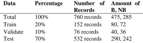
In this experiment, we trained our model with very few data from the dataset to classify a node into either of the two classes: B and NB. Here, B means behaving and NB means not behaving. A behaving node is a good node that is behaving rightly and not causing intentional congestion in the network. On the contrary, a not behaving node is a node that is declared to be harmful based on several features indicated in the dataset. We began the test by seperating 20% data from the preprocessed dataset for training and 10% data for validation using H2O split function. Rest of the data was used for testing performance. Table 2 describes the selection in detail.

Table 2. Dataset split for two class classification taking 20% training data

Data Percentage Number of

Records

Amount of B, NB Total 100% 760 records 475, 285 Train 20% 152 records 80, 72 Validate 10% 76 records 40, 36 Test 70% 532 records 290, 242

After splitting the dataset into train, test and validate set, we applied k-means algorithm on them following the procedure mentioned in the methodology in previous section. Examining the performance of the model on test data, we found that the model predicted the test data with an accuracy of 90.2%. The match-mismatches statistics and the confusion matrix are given in Table 3. The confusion matrix or error matrix (30) is used to find error rate or the classification accuracy in most of the machine learning model. It showed that the k-means algorithm with just 20% training data(152 records) from the preprocessed dataset gives 90.2 percent accurate prediction for two category classification. This result is very significant as it tells that the distribution of the data points in case of two category classification has a uniform separation. This also indicates that k-means is ideal for such dataset classification.

Table 3. Two Class Classification result and confusion matrix for 20% data

Dataset Mislabeled Accuracy Confusion matrix

Test set

(total record= 532, Class B=290, Class NB = 242)

53 out of 532

90.2% Predicted class

0 1 Actual

Class 0 1

263 27 26 216 0 = B, 1 = NB

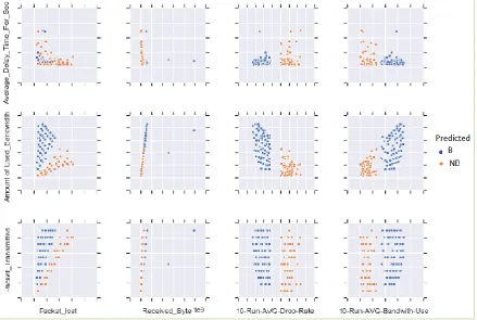
In Fig. 4, a portion of the classification result is plotted for the test dataset. Three attributes

Figure 4. Plot of predicted labels for the test dataset

Three Class Classifications with 20% Data Following the similar steps like two class classification of previous section, we applied the model on three class dataset where the data will be classified into either of B, NB, and PNB label. B and NB classes were discussed in the previous

section. The PNB stands for potentially not behaving. We call a node PNB when it has a mixture of both the behavior of B and NB such that some attribute’s values are similar to B class and some are similar to NB class. Table 4 describes the data splitting in detail.

Table 4. Dataset split for three class classification taking 20% training data

Data Percentage Number of Records Amount of B, NB,

PNB

Total 100% 1075 records 475, 285, 315

Train 20% 215 records 80, 55, 80

Validate 10% 108 records 33, 40, 35

Test 70% 752 records 223, 265, 264

After applying the model, we found that the model predicted the test data with 65.15% accuracy.

The match-mismatches statistics and the confusion matrix are given below in Table 5.

Table 5. Classification result and confusion matrix for 20% data

Dataset Mislabeled Accuracy Confusion matrix

Test set

(total records= 752, Class B=223, Class NB =265, Class PNB=264 )

263 out of 752

65.15%

0 = NB, 1 = PNB, 2 = B Predicted class

0 1 2

Actual class

0 1 2

163 0 102 11 166 87 0 63 160

Four Class Classifications with 20% Data: The original dataset has an attribute called ‘Class’ which has four probable sub-classes, i.e.

Block, No-Block, NB-Wait, and NB-No-Block. The meaning of these four labels is:

Misbehaving node but will not be blocked (NB-No-Block).

Misbehaving node but will not be blocked, will be in waiting state (NB-Wait).

Misbehaving node and will be blocked (Block). In this section, we classified the edge nodes into either of the four above mentioned labels. For

this we replaced the values of ‘Node Status’ attribute in our dataset with the new values from the ‘Class’ attribute of the original dataset. We followed the similar stes as described in previous sections. Table 6 describes the data splitting for this experiment.

Table 6. Dataset split for four class classification taking 20% training data

Data Percentage Number of Records Block, No-Block, NB-No-Block, NB-Wait

Total 100% 1075 records 120, 155, 500, 300

Train 20% 215 records 52, 40, 61, 62

Validate 10% 108 records 23, 40, 19, 26

Test 70% 752 records 213, 155, 299, 85

We found that the model predicted the test data with an accuracy of 41.61%. The

match-mismatches statistics and the confusion matrix are given below in Table 7.

Table 7. Classification result and confusion matrix for 20% data

Dataset Mislabeled Accuracy Confusion matrix

Test set

(Total records= 752, Block= 213, No-Block= 155, NB-No-Block=299, NB-Wait=85)

440 out of 752

41.61%

0=NB-No-Block, 1=NB-Wait, 2= No-Block, 3=Block

Predicted class 0 1 2 3

Actual class

0 1 2 3

137 3 27 132 0 29 20 36 5 52 80 18 40 53 54 66

Through several runs of the algorithm, we found that the k-means gives the mentioned accuracy when trained with 20% training data(215 records) from the dataset.

Summary of the Test Result:

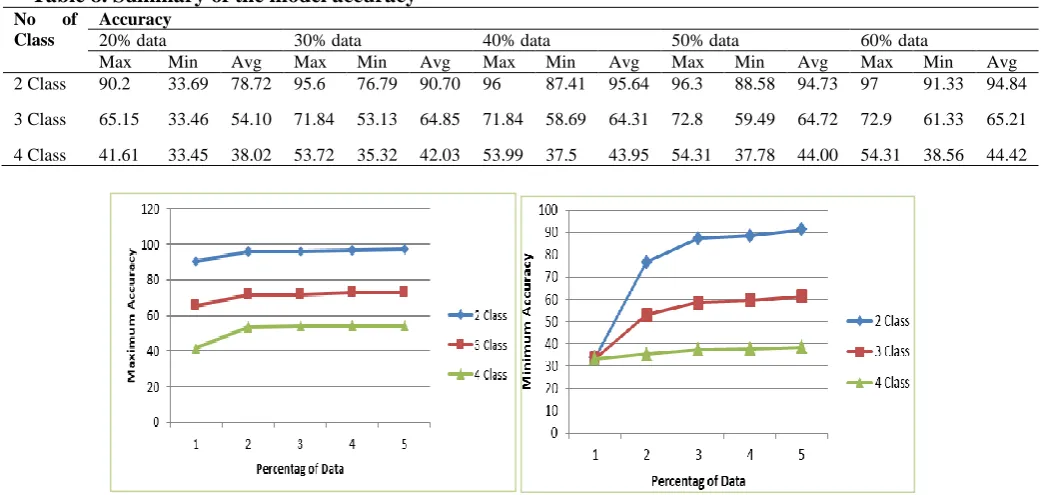
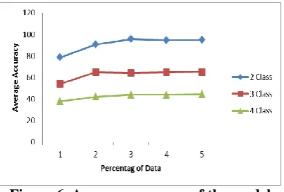
We tested the performance of the constructed model using various sized data, ranging from 20% to 60% for two, three and four classes classification. A summary of the test result is given in Table 8. Below, in Fig. 5, 6 the results are plotted.

Table 8. Summary of the model accuracy No of

Class

Accuracy

20% data 30% data 40% data 50% data 60% data

Max Min Avg Max Min Avg Max Min Avg Max Min Avg Max Min Avg 2 Class 90.2 33.69 78.72 95.6 76.79 90.70 96 87.41 95.64 96.3 88.58 94.73 97 91.33 94.84

3 Class 65.15 33.46 54.10 71.84 53.13 64.85 71.84 58.69 64.31 72.8 59.49 64.72 72.9 61.33 65.21

4 Class 41.61 33.45 38.02 53.72 35.32 42.03 53.99 37.5 43.95 54.31 37.78 44.00 54.31 38.56 44.42

Figure 6. Average accuracy of the model

Comparison of Experimental Results with Related Works:

To the best of our knowledge, there are very few works available on the classification of the nodes in an OBS network using ML techniques. We selected two significant works (7,19) from the

available literatures for a comparison with our work. We discussed about those studies in earlier section. In Table 9, we have given a summary and comparison of these two works with our proposed work.

Table 9. Comparison of the proposed work with related works

Works Type of Work Classification Policy Accuracy (%)

2 Classes 3 Classes 4 Classes

Rajab et.al. (19)

Machine learning: Supervised learning

with 1075 records

If-then rules generated from Decision tree

based model

93 NA 87

Rajab et.al. (7)

Behavior analysis: Computing packet arrival rate and packet

drop rate

Adaptive sliding range window based classifier. Finds the amount of lost burst from each ingress node

during a specific time window

NA

95 percent success rate (with maximum 5% packet drop

rate)

NA

Proposed work

Semi-supervised machine learning

Clustering with K-means algorithm

20% data

30% data

20% data

30% data

20% data

30% data

90.2 95.6 65.15 71.84 41.61 53.72

From Table 9, we see that our model outperforms others in case of two class classification. It is worth repeating that our model predicts with 90.2% accuracy when trained with only 20%(152 records) train data and 10%(76 records) validate data. The model also gives a moderate performance in case of three label classification. But in case of four class classification, it fails to give a satisfactory performance. The reson behind this lower accuracy is that, the K-means algorithm is one of the distance based clustering algorithms that works best with circular/spherical clusters. The dataset we are working with has very irregular shape when four class lebels are considered. That is why such result was not unexpected. This problem can be tackled well by using a clustering algorithm that can deal with arbitrary shaped clusters.

Conclusion:

several ML algorithms and evaluate their performance in detecting malicious nodes. Furthermore, we shall study other types of ML algorithms, i.e. supervised and unsupervised, to be implemented in the context of OBS network security.

Conflicts of Interest: None.

Reference:

1. Coulibaly Y, Al-Kilany AAI, Latiff MSA, Rouskas G, Mandala S, Razzaque MA. Secure burst control packet scheme for Optical Burst Switching networks. In: IBP 2015 - 2015 IEEE International Broadband and Photonics Conference. 2015.

2. Zhu J, Zhao B, Lu W, Zhu Z. Attack-Aware Service Provisioning to Enhance Physical-Layer Security in Multi-Domain EONs. J Light Technol. 2016;34(11):2645–55.

3. Zhu J, Zhao B, Zhu Z. Leveraging game theory to achieve efficient attack-aware service provisioning in EONs. J Light Technol. 2017;35(10):1785–96. 4. Skorin-Kapov N, Chen J, Wosinska L. A new

approach to optical networks security: Attack-aware routing and wavelength assignment. IEEE/ACM T. 2010;18:750–60.

5. Sliti M, Boudriga N. BHP flooding vulnerability and countermeasure. Photonic Netw Commun. 2015;29(2):198–213.

6. Sliti M, Hamdi M, Boudriga N. A novel optical firewall architecture for burst switched networks. In: 12th International Conference on Transparent Optical Networks. 2010. p. 1–5.

7. Rajab A, Huang CT, Alshargabi M, Cobb J. Countering burst header packet flooding attack in optical burst switching network. In: International Conference on Information Security Practice and Experience. Springer International Publishing; 2016. p. 315–329.

8. Sheikhpour R, Sarram MA, Gharaghani S, Chahooki MAZ. A Survey on semi-supervised feature selection methods. J Pattern Recognit. 2017;64:141–58. 9. Zhu X. Semi-Supervised Learning Literature Survey.

SciencesNew York. University of Wisconsin-Madison; 2005.

10. Arora P, Deepali, Varshney S. Analysis of K-Means and K-Medoids Algorithm for Big Data. In: International Conference on Information Security & Privacy. 2016. p. 507–512.

11. Wu J, Liu H, Xiong H, Cao J, Chen J. K-means-based consensus clustering: A unified view. IEEE Trans Knowl Data Eng. 2015;27(1):155–69.

12. Dubey AK, Gupta U, Jain S. Analysis of k-means clustering approach on the breast cancer Wisconsin dataset. Int J Comput Assist Radiol Surg. 2016;11(11):2033–47.

13. He H. A Network Traffic Classification Method Using Support Vector Machine with Feature

Weighted-degree. J Digit Inf Manag. 2017;15(2):76– 83.

14. Wang Y, Li D, Du Y, Pan Z. Anomaly detection in traffic using L1-norm minimization extreme learning machine. Neurocomputing. 2015;149:415–25. 15. Wang M, Cui Y, Wang X, Xiao S, Jiang J. Machine

Learning for Networking: Workflow, Advances and Opportunities. IEEE Netw. 2018;32(2):92–9.

16. Moore AW, Zuev D. Internet traffic classification using bayesian analysis techniques. ACM SIGMETRICS Perform Eval Rev. 2005;33(1):50–60. 17. Jayaraj A, Venkatesh T, Murthy CSR. Loss Classification in Optical Burst Switching Networks using Machine Learning Techniques: Improving the Performance of TCP. IEEE J Sel Areas Commun. 2008;26(6):45–54.

18. Levesque M, Elbiaze H. Graphical Probabilistic Routing Model for OBS Networks with Realistic Traffic Scenario. In: IEEE Global Telecommunications Conference. 2009. p. 1–6. 19. Rajab A, Huang CT, Al-Shargabi M. Decision tree

rule learning approach to counter burst header packet flooding attack in Optical Burst Switching network. Opt Switch Netw [Internet]. 2018;29:15–26.

Available from:

https://doi.org/10.1016/j.osn.2018.03.001

20. Forgy E. Cluster Analysis of Multivariate Data: Efficiency versus Interpretability of Classification. Biometrics. 1965;21:768–780.

21. Blömer J, Lammersen C, Schmidt M, Sohler C. Theoretical analysis of the k-means algorithm–A survey. Algorithm Eng. 2016;81–116.

22. UCI. BHP flooding attack on OBS Network Data Set [Internet]. Available from: https://archive.ics.uci.edu/ml/datasets/Burst+Header+ Packet+%28BHP%29+flooding+attack+on+Optical+ Burst+Switching+%28OBS%29+Network#

23. NCTUns Network Simulator and Emulator [Internet].

Available from:

http://nsl.cs.nctu.edu.tw/NSL/nctuns.html

24. H2O.ai [Internet]. Available from: http://www.h2o.ai/

25. Python programming language [Internet]. Available from: https://www.python.org/

26. Lever J, Krzywinski M, Altman N. Points of Significance: Model selection and overfitting. Nature Methods. 2016. p. 703.

27. Koo TK, Li MY. A Guideline of Selecting and Reporting Intraclass Correlation Coefficients for Reliability Research. J Chiropr Med. 2016;15(2):155–63.

28. Splitting Datasets into Training/Testing/Validating [Internet]. Available from: http://h2o- release.s3.amazonaws.com/h2o/master/3545/docs-website/h2o-docs/datamunge/splitdatasets.html 29. Dziak JJ, Coffman DL, Lanza, ST, Li R, Jermiin LS.

Sensitivity and specificity of information criteria. The Methodology Center and Department of Statistics, Penn State. 2018.

ةيمزراوخ مادختساب فارشلإل يلآ هبش يميلعت جهنم

K-Means

عافدنلاا سأر مزح ةمزح قفد موجه عنمل

ةيرصبلا تاراجفنلاا ليدبت ةكبش يف

يروتاب نيسح رمق دمحم

قحلا لماك دمحم

ةسدنهلل جنوجاتيش ةعماج ، رتويبمكلا ةسدنهو مولع مسق جنوجاتيش ، ايجولونكتلاو

-4349 شيدلاغنب ،

لا

:ةصلاخ

يرصبلا عافدنلاا ليدبت ةكبش (OBS)

ةكبش يف .ديدجلا ليجلا نم يرصب لاصتا ةينقت يه OBS

ةمزح ًلاوأ ةفاحلا ةدقع لسرت ،

عافدنلاا سأر ةمزح ىمست ، مكحت (BHP)

ةمداقلا تانايبلا ةعفدل ةمزلالا دراوملاب ظفتحت يتلا (DB).

ب ةدعاق أدبت ، زجحلا لامتكا درجم

ةكبش ىلع زراب موجه كانه .زوجحملا راسملا للاخ نم اهتهجو ىلإ كرحتلاب تانايبلا OBS

ناضيف موجه وه BHP

ةدقع لسرت ثيح

ةفاحلا BHPs دراوملا رادهإ متي ، كلذل ةجيتن .اهب ةطبترملا تانايبلا ةدعاق لسرت لا عقاولا يف نكلو ، دراوملا زجحل ثدحي امدنعو ةزوجحملا

ةمدخلا ضفر ثدحي دقف ، ةيافكلا هيف امب عساو قاطن ىلع كلذ (DoS).

ةيمزراوخ مادختساب ملعتلل ةيلآ هبش ةقيرط حرتقن ، ثحبلا هذه يف

لئاسولا k ةكبش يف ةثيبخلا دقعلا فاشتكلا ، OBS.

يب مادختساب هتحص نم ققحتلاو حرتقملا بقارملا هبش جذومنلا بيردت مت ةريغص ةيمك تانا

ةقدب فرصتت لا وأ فرصتت لوصف ىلإ دقعلا فنصي نأ نكمي جذومنلا نأ براجتلا رهظُت .ةراتخم تانايب ةعومجم نم 90

بيردتلا دنع ٪

مادختساب 20 ةقد رهظي جذومنلا نإف ، فرصتت لا امبرو ،فرصتت لا ، فرصتت لوصف ىلإ دقعلا فينصت متي امدنع .تانايبلا نم طقف ٪

65.15 و ٪ 71.84 ةبسنب هبيردت مت اذإ ٪ 20

و ٪ 30 جذومنلا نأ تفشك ةزرابلا لامعلأا ضعب عم ةنراقم .يلاوتلا ىلع تانايبلا نم ٪

يحاونلا نم ريثك يف اهيلع قوفتي حرتقملا .

:ةيحاتفملا تاملكلا

ةيمزراوخ ، ةدمعلأا سوؤر مزح ناضيف موجه K-Means

ليدبت ةكبش ، يللآا ملعتلا ، هبش ملعتلا ، ةيرصبلا تاراجفنلاا