https://doi.org/10.5194/os-14-783-2018
© Author(s) 2018. This work is distributed under the Creative Commons Attribution 4.0 License.
Acoustic Doppler current profiler observations of migration patterns
of zooplankton in the Cretan Sea
Emmanuel Potiris1,2, Constantin Frangoulis1, Alkiviadis Kalampokis1, Manolis Ntoumas1, Manos Pettas1, George Petihakis1, and Vassilis Zervakis2
1Institute of Oceanography, Hellenic Centre for Marine Research, Heraklion, Crete, 72100, Greece
2Department of Marine Sciences, School of the Environment, University of the Aegean, Mytilene, Lesvos, 81132, Greece
Correspondence:Emmanuel Potiris ([email protected])
Received: 31 January 2018 – Discussion started: 13 February 2018 Revised: 8 June 2018 – Accepted: 6 July 2018 – Published: 9 August 2018
Abstract. The lack of knowledge of the mesopelagic layer inhabitants, especially those performing strong vertical mi-gration, is an acknowledged challenge. This incomplete rep-resentation leads to the exclusion of an active carbon and nutrient pathway from the surface to the deeper layers and vice versa. The vertical migration of mesopelagic inhab-itants (macroplanktonic and micronektonic) was observed by acoustical means for almost 2.5 years in the epipelagic and mesopelagic layers of the open oligotrophic Cretan Sea (south Aegean Sea, eastern Mediterranean) at the site of an operational fixed-point observatory located at 1500 m depth. The observed organisms were categorized into four groups according to their migration patterns. The variability of the migration patterns was inspected in relation to the physical and biological environmental conditions of the study area. The stratification of the water column does not act as a barrier for the vertical motion of the strongest migrants that move up to 400 m every day. Instead, changes in light intensity (lunar cycle, daylight duration, cloudiness) and the presence of prey and predators seem to explain the observed daily, monthly and seasonal variability. The continuous presence of these organisms, which are capable of vertical motion despite the profound circulation variability at the site of the observatory, implies their presence in the broader study area. The funda-mental implications of the above regarding biogeochemical processing in oligotrophic seas due to the intimate link be-tween the carbon (C) and nutrient cycles, are discussed.
1 Introduction
The biological organic carbon pump is the major oceanic process that photosynthetically converts the dissolved CO2 in the surface layers of the ocean to particulate organic car-bon. This organic carbon is then consumed by pelagic biota, and exported to depth by a combination of sinking parti-cles, advection or vertical mixing of dissolved organic mat-ter and transport by animals (Turner, 2015). Buesseler and Boyd (2009) noted that “the surface ocean” is “where the “strength” of the biological pump is set” whereas “the sub-surface ocean” is “where the “efficiency” of the biological pump is determined”.
to explain some cases where DVM occurs at depths below 1000 m, where light cannot penetrate (van Haren, 2014, and references therein).
There are also still gaps in the knowledge regarding mid-water depths, which severely limit our ability to quantify the efficiency of the biological pump (Robinson et al., 2010). Concerning zooplankton DVM, one of the methodologi-cal limitations is that the populations of large individuals (macrozooplankton) that belong to important and common predatory groups capable of strong migrations, such as the chaetognaths, amphipods, euphausiids, decapods, have been underestimated. This is due to the fact that many of them escape the standard 200 µm mesh size net when towed at the recommend speed of less than 1 m s−1 (Moriarty and O’Brien, 2013). However, such large individuals can be de-tected by low frequency Acoustic Doppler current profilers (ADCPs hereafter).
Progress in ocean acoustics and marine technology during the early 1980s (Costello et al., 1989; Holliday, 1977; Holl-iday and Pieper, 1980; HollHoll-iday et al., 1989) allowed for the estimation of distribution patterns and biomass of zooplank-ton and micronekzooplank-ton to be inferred from ADCPs (Flagg and Smith, 1989). To measure currents, ADCPs transmit sound pulses in different directions. The sound is scattered by par-ticulate matter in the water column, and radial velocities are computed from the Doppler shift of the backscattered sig-nal (Gordon, 1996). The intensity of the backscattered sound can also be used in conjunction with net samples for estimat-ing the biomass of zooplankton (Ashjian et al., 2002). Whilst the estimated ADCP backscatter is a by-product (Bozzano et al., 2014), meaning that it is more suitable for qualitative than quantitative analysis (Brierley et al., 1998), field stud-ies complemented with ADCP-derived sound scattering have been used to describe biological patterns in the interior of the ocean, such as zooplankton aggregations (Zhou and Dorland, 2004) and vertical migration (Postel et al., 2007), in remark-able detail.
In the Mediterranean Sea, there have been several studies on vertically migrating zooplankton (see Table 5 in Ander-sen et al., 2001), and some have shown a substantial contri-bution to the total carbon export in deep waters via the ac-tive transport of migrants (Isla et al., 2015, and references therein). However, these Mediterranean DVM studies have mainly been based on net sampling for short total sampling periods (e.g., discontinuous sampling at a monthly frequency or continuous sampling for a few weeks). It is worth noting that studies of macrozooplankton are far less common than those regarding mesozooplankton, and that even for meso-zooplankton there are very few interannual-scale studies in the open Mediterranean Sea (Siokou-Frangou et al., 2010). Among the Mediterranean DVM studies, the majority has been centered in the western Mediterranean (see Table 5 in Andersen et al., 2001; review by Saiz et al., 2014). These studies have pointed out different species-dependent migrat-ing strategies, with some species migratmigrat-ing upwards and
oth-ers downwards at night, as well as a within species age–depth and sex–depth differential distribution. These observations were made in both the eastern and western Mediterranean (Andersen et al., 2001; Fragopoulu and Lykakis, 1990). The only DVM study in the Cretan Sea (Heraklion Bay) upper slope (300 m sea bottom) studied near-bottom macrozoo-plankton, and reported a reversed DVM, i.e., downward mi-gration during nighttime (Koulouri et al., 2009).
The Cretan Sea is the most voluminous and deep (2500 m) basin of the Aegean Sea and an area of intense mesoscale variability and multiple scale circulation patterns. Two mesoscale gyres form a dipole in the Cretan Sea (Cardin et al., 2003; Kassis et al., 2015; Theocharis et al., 1999), while it is also an area of intermediate and/or deep-water for-mation (review by Skliris et al., 2014). Such areas of wa-ter formation are key locations for the monitoring of the Mediterranean biochemical functioning (Malanotte-Rizzoli et al., 2014). Modeling studies have shown that the open Cre-tan Sea’s biochemistry is representative of a wide area of the eastern Mediterranean varying from 0.6 to 1.6×10⁶km2 de-pending on the variable (i.e., primary production – PP, sea surface temperature – SST, pH, O2, NO3, chlorophyll a) (Henson et al., 2016).
Satellite (SeaWiFS) studies of chlorophylla(Chla) have clustered the Cretan Sea in a wider bioprovince of the south-central and eastern Mediterranean that covers 60 % of the total Mediterranean area, and is generally characterized by oligotrophic conditions (D’Ortenzio and Ribera d’Alcalà, 2009). The presence of a deep chlorophyll maximum (DCM hereafter), a common Mediterranean feature, which deepens going eastwards (e.g., Lavigne et al., 2015; Nowaczyk et al., 2011), also characterizes the Cretan Sea and depends on the close coupling of biological and physical processes. In fact, whilst the DCM’s magnitude is mainly determined by bio-logical mechanisms, the DCM depth and structure are essen-tially determined by optical–physical factors (e.g., Crise et al., 1999; Mann and Lazier, 2006; Varela et al., 1994). In the Cretan Sea the vertical extent and the intensity of the mesoscale gyres, which form a dipole, govern this coupling to a large extent (Petihakis et al., 2002).
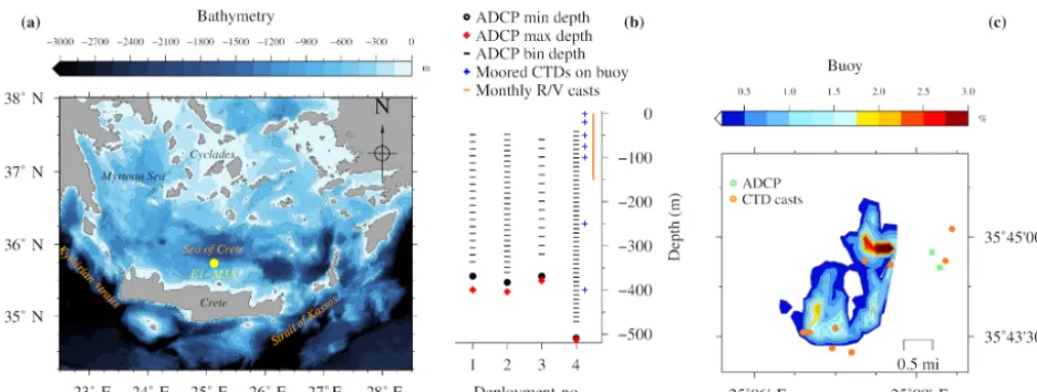
Figure 1.Topographic map of the south Aegean Sea(a). Vertical(b)and horizontal(c)views of the sampling setup at E1-M3A. Details of ADCP deployments are given in Table 1. Horizontal buoy motion is shown as a percentage of the total deployment duration spent at a location.
living macrozooplankton there is even less information. The euphausiid species found in the whole Mediterranean Sea are the same, although the predominant species are differ-ent in the eastern basin and Thyrrenian Sea to those found in the western basin, west of the Thyrrenian Sea (Wiebe and D’Abramo, 1972).
ADCP studies of DVM in the Mediterranean have been limited. In the central Ligurian Sea, Bozzano et al. (2014) used an upward looking ADCP positioned at a depth of 100 m. They found that the main migration pattern is the daytime migration, in addition to the fact that deeper and stronger migration ranges are encountered during winter. In the Alboran Sea, van Haren (2014) implemented an upward looking ADCP positioned at a depth of approximately 800 m and found DVM to be related to internal waves. To our knowledge, there have been no ADCP studies of DVM in the eastern Mediterranean. However, during a study of the cur-rent velocities in the Cretan Sea in 2000, Cardin et al. (2003), using an ADCP (75 kHz), reported a noise in the measure-ments of vertical velocity, and migrating zooplankton was given as a possible explanation.
The present study was stimulated by this hypothesis from Cardin et al. (2003), in addition to the fact that for the 75 kHz frequency objects with a size of 5 mm (1/4 of trans-mit pulse wavelength) or more reflect sound and cause a strong backscatter signal (Thomson and Emery, 2001). Fol-lowing this hypothesis, four consecutive deployments of the same 75 kHz ADCP were carried out at the same location as Cardin et al. (2003), covering a period of two and a half years. This provided a unique opportunity to study the migra-tion patterns of zooplankton, continuously and at high fre-quency, for a long period in relation to environmental condi-tions. The aim of this paper is to present the observed dis-tribution patterns of zooplankton (focusing on DVM) and discuss their relationship to physical and biological
environ-mental conditions, such as daylight, currents, stratification and food resources.
2 Materials and methods 2.1 Experimental setup
Table 1.The deployment parameters of the upward looking 75 kHz RDI ADCP on the subsurface mooring line of E1-M3A.
Deployment Start End Bins Bin size Sampling interval First bin Average depth
(m) (s) (m) (m)
First 15 Nov 2012 23 May 2013 25 16 1800 24.59 369 Second 1 Jun 2013 19 Jan 2014 33 12 3600 20.65 383 Third 19 Jan 2014 10 Oct 2014 25 20 1800 28.58 370 Fourth 10 Oct 2014 2 Jun 2015 45 10 1800 18.76 509
only the last ADCP deployment was about 120 m deeper than the previous deployments.
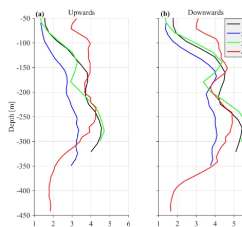
The ADCP sampling plan was optimized in terms of tem-poral and spatial resolution by setting different sampling schemes at each deployment (Table 1; Fig. 1b). The aim was to check the consistency of the vertical velocity measure-ments of zooplankton and the backscatter coefficient (defined in Sect. 2.2) between deployments. No significant difference in the vertical velocities or the backscatter coefficient be-tween deployments of variable cell length and sampling rate, is an indication of reliable/accurate measurements. Thus, it is possible to identify biases caused by the sampling scheme, instead of the velocity errors due to the ADCP accuracy and the backscatter coefficient estimation methodology.
One parameter used to potentially identify the optimal cell extension and sampling interval for the most appropri-ate recording of zooplankton signals was the hereafter de-fined “burst speed”. The burst speeds of each cell are dede-fined as the highest and lowest vertical velocity measurements, re-spectively, during a one day time period. The velocity mea-surement inside a cell over the sampling interval is the result of the averaging of several pings. As the recording interval increases, the cell extension decreases and the actual zoo-plankton speed increases; we expect the actual zoozoo-plankton speed to be underestimated because zooplankton will not be inside the cell throughout the duration of the measurement, only during a fraction of it. The largest underestimation is ex-pected when the actual zooplankton migration speed is at its maximum. Thus, comparison of upward and downward burst velocities between deployments at depths around 250 m (the depth at which the highest migrating speeds were recorded) were used to identify the most appropriate sampling scheme. The challenge was to identify the lowest sampling rate that would still give an acceptable resolution for the as-cending/descending zooplankton movement, while conserv-ing power and extendconserv-ing the deployment period as much as possible. Two sampling and averaging intervals, of 30 min and 1 h, respectively, were tested in order to select the opti-mum sampling scheme. During the first deployment, a sam-pling interval of 30 min was used, which was subsequently followed by a 1 h interval during the second deployment. Comparison of the data from the two deployments revealed an underestimation of burst migration velocities in the sec-ond data set (Fig. 2a and b) due to the lower sampling rate
Figure 2.Time average burst velocities per ADCP deployment.
(1 h); thus, the initial value of 30 min was selected for the last two deployments.
In comparison, the range of the cells used (10–20 m) did not affect the burst speed or the average velocity measure-ments. Based on visual inspection, smaller cell extension during the first, third and fourth deployments (30 min sam-pling interval) did not result in smaller burst and average speeds. However, using a small bin size (10 m) during the last deployment resulted in noisy velocity measurements. The depth-integratedSv (backscatter coefficient, defined in
Sect. 2.2) between the depths observed for all deployments were also consistent. The seasonal variability of the physical properties of the water column affected the estimation ofSv
2.2 Data processing/analysis and visualization of backscatter data
The backscatter coefficientSvdBre 4πm−1is given as
follows:
Sv=C+10log10
(Tx+273.16) R2
−LDBM−PDBW +2aR+Kc(E−Er) , (1) whereC(dB)= −159.1 is an instrument constant,Tx(◦C) is
the transducer temperature,R (m) is the slant range,LDBM is the 10log10of the transmit pulse length (m),PDBWis the 10log10of the transmit power (W),a (dB m−1) is the sound absorption coefficient,Kcis a constant of proportionality for converting the incoming raw echo data to dB,E(counts) is the raw echo data andEr=min(E)(counts) is the reference raw echo per transducer when there is no signal.Svwas
cal-culated according to Deines (1999), Kc according to Hey-wood (1996), the speed of sound for the calculation of R
according to Gordon (1996) andaaccording to Ainslie and McColm (1998).
Instantaneous vertical velocity profiles were depth aver-aged and split into daily data sets to identify the hours of the day during which the zooplankton move upward or down-ward, as well as the seasonal and interannual variability in the ascent/descent hours. Another step was to select the max-imum and minmax-imum vertical velocities of each daily piece of data during the periods of upward and downward move-ment. Depending on the sampling rate, two to four samples were averaged. Finally, histograms of vertical velocity versus depth one hour before and one hour after sunrise/sunset were used to identify possible ascending/descending differences of migration patterns and evaluate the consistency between the different ADCP sampling schemes.
Climate Data Operators (CDO, 2018), Ocean Data View (Schlitzer, 2016) and Generic Mapping Tools (Wessel et al., 2013) were used for the data processing and visualization. Wind stress and sensible/latent fluxes were computed from the quality-controlled buoy data with the “air-sea” toolbox to identify the time when conditions favor the overturning of the water column (http://woodshole.er.usgs.gov/operations/ sea-mat/air_sea-html/index.html, last access: 25 July 2018). 2.3 Description and processing of auxiliary data To estimate volume backscattering, assess environmental conditions during deployments and assist with the interpre-tation of ADCP measurements, several complementary data sets have been used (Table 2).
The E1-M3A buoy measures meteorological variables (wind speed, gust and air temperature were used here) as well as temperature, conductivity and fluorescence at multi-ple depths (20, 50, 75 and 100 m). Temperature and conduc-tivity measurements are also available at the sea surface and at a depth of 250 m. The chlorophyll concentrations are mea-sured with the WETLabs ECO FLNTU fluorescence sensors
which are mounted on the moored 16plus CTDs. A down-ward looking Nortek 400 kHz ADCP is mounted to the buoy hull, measuring horizontal currents at 5 m bins from the sur-face down to a depth of 50 m. Due to the lack of compatibility between the 400 kHz ADCP and the buoy software, backscat-ter measurements are not available from this instrument. The above meteorological and marine surface parameters were downloaded from the Poseidon online database (http://www. poseidon.hcmr.gr, last access: 25 July 2018), where they are stored in real time. In addition, due to occasional problems with the real-time underwater transmission, subsurface sen-sor data were downloaded from the memory logs of the in-struments during the regular biannual maintenance. Mete-orological and sea surface measurements from the buoy’s sensors span a period of 24 months (from 22 May 2013 to 25 May 2015) and subsurface measurements a period of 20 months (from 22 May 2013 to 10 January 2015). Buoy data have undergone automated quality control, such as the rejection of stalled values and the application of min–max and spike filters. Visual inspection was the last quality con-trol step; the remaining suspect measurements were removed manually. The heat flux through the air-sea interface compu-tations were based on the air-sea interaction Matlab routines provided by Rich Pawlowitz (via the SEAMAT collection, https://sea-mat.github.io/sea-mat/, last access: 25 July 2018), applied on the E1-M3A meteorological and sea surface data.
2.4 Limitations
Several limitations of the ADCP and auxiliary data should be carefully considered.Svis a proxy for zooplankton biomass
and when integrated along the acoustical beams it can pro-vide a gross measure of the instantaneous biomass of the water column (changes in the acoustical character of zoo-plankton cannot be identified). Whilst the integratedSv is
consistent among the deployments (discrepancies between deployments were only observed for the first few bins), an analysis of this description is not meaningful with the exper-imental configuration of this study. This is due to the fact that the zooplankton are not permanently within the range of the ADCP and because of the seasonal succession of dominant species constituting the zooplankton stocks in the Cretan Sea (Gotsis-Skretas et al., 1999). The upper 50 m of the water column are not measured, which means that the depth inte-gratedSvexhibits significant variability due to the monthly
change in the depth to which the zooplankton ascend dur-ing nighttime because of moonlight. Furthermore, the whole deep scattering layer is only found inside the ADCP range for a small period of the fourth deployment, adding another source of variability that is not attributed to biomass changes of zooplankton. Another source of error, which largely de-pends on the availability of auxiliary data, is the imperfect calculation of the effects of the gradients of the upper water column in the estimation ofSv due to the changes in
en-Table 2.The type, source, time coverage and resolution of the auxiliary data. In situ data have gaps of variable lengths. Monitoring by R/V refers to the monthly monitoring program of regular R/V visits to the E1-M3A observatory site. NASA refers to the Goddard Space Flight Center.
Parameter Type Source Time coverage Time
reso-lution
Air temp & wind In situ E1-M3A buoy 2013/05–2014/10 3 h
Surface currents (0–50 m) In situ E1-M3A buoy (ADCP 400 kHz)
2013/05–2015/05 3 h
Subsurface currents (0–400 m) In situ ADCP (75 kHz) 2012/11–2015/05 0.5–1 h
Water temperature & salinity In situ In situ Reanalysis
E1-M3A buoy
Monitoring by R/VSeaDataNet
2013/05–2015/01 2010/03–2015/01 Climatology
3 h 1 m 1 m
Chla In situ
In situ
E1-M3A buoy Monitoring by R/V
2013/05–2014/06 2010/03–2015/05
3 h 1 m
Cloud fraction & optical thickness Satellite NASA 2015/02–2015/03 1 d
countered when measuring zooplankton with upward look-ing ADCPs and should be treated with caution in acoustical studies of zooplankton.
2.5 Hydrology of the Cretan Sea
The ADCP site is located at the center of the semi-permanent dipole of the Cretan Sea, which consists of a cyclone to the east and an anticyclone to the west of the observatory (Korres et al., 2014; Theocharis et al., 1999). Low frequency variabil-ity at the study site is controlled by the intensvariabil-ity and the ver-tical extent of the dipole as reported by Cardin et al. (2003). Four water masses fill the surface and subsurface layers of the Cretan Sea. Modified Atlantic Water (MAW, salinity (S)=38.5–38.9 psu) fills the 20–100 m layer. Cretan Inter-mediate Water and Levantine InterInter-mediate Water, which have similar characteristics (CIW & LIW, potential temperature (θ )=14.9–15.1◦C, S∼39.0–39.1 psu) fill the 200–500 m layer. Transitional Mediterranean Water (TMW,θ=14.2◦C,
S=38.92 psu), a mixture of Levantine Intermediate Water and Eastern Mediterranean Deep Water enters through the Cretan straits and its core lies at the 500–800 m layer (Geor-gopoulos et al., 2000; Velaoras et al., 2013) or deeper (Ve-laoras et al., 2015). Below the TMW lies the Cretan Deep Water, a water mass argued to have local (Theocharis et al., 1999) or north/central Aegean origin (Gertman et al., 2006; Zervakis et al., 2000). Inflow of Atlantic water (Theocharis et al., 1999), typically during late summer, causes a salinity minimum at the subsurface layer.
3 Results
3.1 Environmental conditions at the study site
Sea surface temperature ranged seasonally from 15 to 26◦C and salinity ranged from 38.8 to 39.5 psu (Fig. 3b and c). The salinity of the deeper layers ranged from 38.9 to 39.1 psu. The lowest temperatures were observed during February and March, while the highest temperatures were seen during Au-gust and September. The seasonal cycle of temperature pen-etrated down to 100 m and the permanent thermocline ex-tended down to 350 m (Fig. 3b). Salinity also exhibited a sea-sonal cycle down to 100 m, but the seasea-sonal signal dominated the salinity variations of the upper part of the water column (Fig. 3c). The highest salinity values were observed during calm, cloud free summer days. A salinity minimum between the surface and 100 m depth was also observed in Fig. 3c. Deep casts (Fig. 3e and f) revealed a continuous change of the water column towards fresher and colder values between 250 and 1000 m, especially from 2012 to 2016, which points to intensified horizontal motion of the subsurface layers. The temperature at the depth of the deep scattering layer around 450 m (based on the available data set; Fig. 3d, e and f), ranged from 14.55 to 14.9◦C and the salinity from 38.98 to 39.04 psu.
com-Figure 3.CTD casts collected during monitoring and maintenance visits to the E1-M3A observatory site with HCMR research vessels from 2010 to 2016. Time–depth plots of potential density anomalies (σ0)(a), potential temperature (θ)(b)and practical salinity (S)(c).θ–S plot(d)and vertical profiles ofS(e)andθ(f)are colored according to the date to reveal temporal trends.
plete data set was 0.082 Pa). Wind stress during December 2013 was more than 0.2 Pa on average, while peak values of 0.8 Pa were also observed. Consequently, the monthly aver-age sensible heat flux was about 100 W m−2 and peak val-ues were about 300 W m−2. Latent heat during that period peaked at 600 W m−2. Similar atmospheric conditions that favored convection of the upper 100 m of the water column were observed from 10 to 22 February 2015.
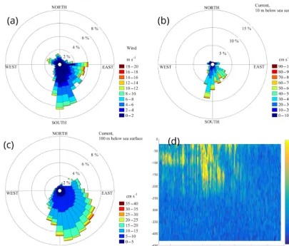
Average water velocity from the surface down to 50 m was 0.29 m s−1towards the south-southeast and was invari-ant with depth. The layer between 50 and 350 m depth was characterized by a diminishing vertical shear that was largest between a depth of 50 and 150 m and vanished below 400 m (Fig. 4d, where only the fourth deployment is displayed, since the larger bin size had caused an underestimation of the high vertical wavenumber shear in previous deployments). The average current speed below 350 m was 0.06 m s−1. The direction of the axis of maximum variance between the sur-face and 50 m was south-southeast and gradually turned to south-southwest at 200 m depth. Currents were also less uni-directional with depth. The strong currents of the surface layer exhibited the least directional variability (Fig. 4b and c). High frequency variability at the site consisted of iner-tial and tidal currents, which accounted for a small portion
of the total variance (less than 8 %) even though the inertial motions were dominant over short periods.
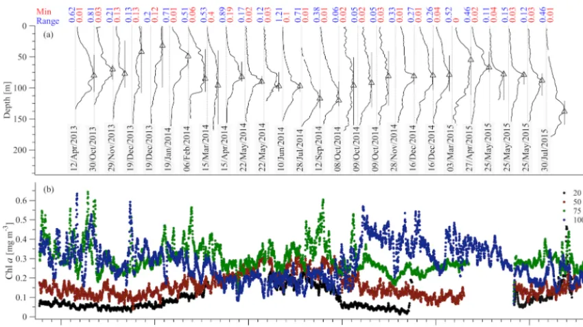
During the study period the core of the DCM was observed between 70 and 120 m and its vertical extent was around 60 m (Fig. 5a). On average, the largest chlorophyll values were observed at the buoy’s 75 and 100 m sensors (Fig. 5b). Furthermore, at these depths, the short-term variability was comparable to the variability due to the annual cycle, while for the 20 and 50 m sensors the seasonal variability was dom-inant. The DCM formed from February to April and was usu-ally destroyed by October (see changes of the depth range for which the chlorophyll concentration is above 70 % of the maximum value in Fig. 5a).
Figure 4.Rose diagrams of wind(a)and surface (10 m depth) currents from the buoy’s ADCP (400 kHz downward looking)(b), subsurface currents at 100 m depth from the upward looking 75 kHz ADCP(c)and vertical shear from the fourth deployment(d). The direction in panels (a),(b)and(c)point to the direction of the flow.
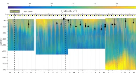
A closer examination of daily backscatter patterns (Fig. 7) allowed for the categorization of the scattering organisms into four groups according to their migration patterns; this was undertaken on the basis of distinguishable trails of vol-ume backscatter measurements from the ADCP. Three of the groups exhibited a daily migrating pattern, while the fourth remained at a constant depth. The first group (group A here-after) did not migrate. It was found at 400–450 m, and it formed a deep scattering layer (Fig. 7c).
Group B (Fig. 7) followed the normal DVM pattern, i.e., it moved close to the surface at dusk and returned to the park-ing depth at dawn, where it stayed durpark-ing the day. This group spent the daytime at a depth of 400–450 m and the nighttime between 150 m and the surface (Fig. 7). When at the bottom of the seasonally varying daytime parking layer (60–160 m), its vertical velocity decreased; however, it was still moving towards the surface. The bottom of the daytime parking layer was identified by the deceleration of upward movement and the subsequent increase of Sv (Fig. 7), as the zooplankton
spent more time in a particular cell when moving at a lower
speed. The change in the depth of the bottom of the day-time parking layer of group B was in good agreement with the time variation of the depth of the maximum chlorophyll concentration.
The backscatter coefficient at any certain depth, as long group B was above that depth, was larger during nighttime than daytime (Fig. 7). The exception to this rule was the deep scattering layer. The result was the “curtain” shape ofSvseen
in Fig. 7, which implies that a part of the zooplankton that form group B spread through the entire 50–400 m water col-umn while migrating. The smallest Sv values, close to the
system noise floor, were observed between 250 and 300 m, when group B was found at the parking depth.
Between 300 and 350 m,Sv never fell close to the noise
Figure 5.Chlorophyll concentration from the CTD casts(a)and the E1-M3A CTD sensors(b). The casts show the vertical distribution of the chlorophyll concentration in the water column (normalized, solid black lines). The minimum value of each cast is denoted by the vertical grey line and the maximum value of each cast is denoted by the black triangle. The black bars around the triangles denote the depth range for which the chlorophyll concentration is above 70 % of the maximum value of the cast. The minimum value and the range of the original chlorophyll values (in mg m−3) are shown above each cast in red and blue, respectively. The E1-M3A chlorophyll data are low passed with a one-day running mean filter.
At shallower depths a fourth group was observed (Fig. 7, Group D), which spent most of the daytime at a depth be-tween 180 and 240 m and during the night it moved to more shallow depths of between 60 and 90 m, where its trails met with those of group B. This was close to the depth where the layer with the largest concentration of phytoplankton throughout most of the year was observed. The backscatter signal of group D was not as strong as that of group B; how-ever, its trail was generally easily distinguishable during its period of upward motion, as a secondary thin strongSvtrail,
shallower than the one caused by group B; this was less ob-vious during the downward motion (Fig. 7). This signal was present in all deployments, but not throughout each deploy-ment, and its characteristics, such as depth and slope, were consistent between deployments.
3.3 Migration timing, duration and velocity
The duration of strong migration did not change with time, with two hours spent each way (four hours in total) (Fig. 8a). Descent was symmetrical with respect to the sunrise; it started one hour before and ended one hour after sunrise (Fig. 8a). Ascent started half an hour before and ended one and a half hour after sunset (Fig. 8a). Depth-averaged veloc-ities during the strong migration period were about 3 cm s−1. While the duration of the strong migration was constant, the migrating velocity changed seasonally, following the
dura-tion of the day which, at 35◦longitude, lasts 9.8 h on winter solstice and 14.5 h on summer solstice. This is clearly shown in Fig. 8b, despite the fact that the velocities are quite noisy. Downward velocity was slightly higher than the upward ve-locity – by almost 1 cm s−1on average (Fig. 8b).
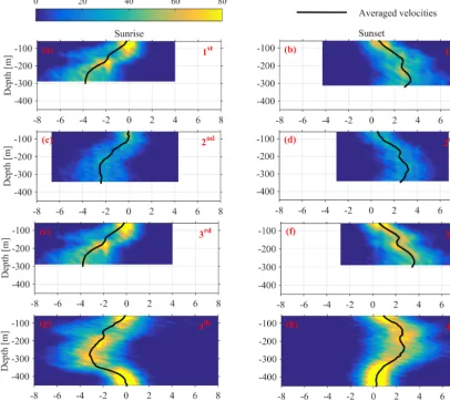
Monthly variability was observed at the depths at which strong downwards migration started (speeds higher than 2.5 cm s−1)(Fig. 9). Furthermore, in Figs. 9 and 10 it can be seen that zooplankton did not migrate at a constant ve-locity with depth. The highest upward velocities, close to 6 cm s−1were recorded between 200 and 300 m. The highest downward velocities were recorded between 250 and 350 m (Fig. 10). Since group B traveled the longest distance in the course of a day, the largest vertical velocities recorded, espe-cially between 200 and 350 m, might be due to the migration of group B. At a depth of 200 m the ADCP recorded rela-tively small vertical velocities, about 2 cm s−1(Figs. 9 and 10, all panels), which distorted the vertical profile that would be expected from group B, unless group B decelerated at the bottom of the photic zone. The dispersion of the vertical ve-locity around the average value at that depth was much less than all the other depths (Fig. 10, all panels).
It was not possible to distinguish the velocity of group B from the velocity of group C, as their Sv trails overlapped
during migration. However, utilizing theSvtrails attributed
Figure 6.The backscatter coefficient for all ADCP deployments is shown. The beginning of a year is denoted by a dashed vertical line. The yellow and black circles denote the dates of the full and new moons, respectively. The maximum chlorophyll value of available casts is denoted by the black triangle. The gray bars around the triangles represent the depth range for which the chlorophyll concentration is above 70 % of the maximum value of the cast.
Figure 8.Instantaneous depth-averaged vertical velocities of daily segments of ADCP measurements between 350 and 50 m(a), following Jiang et al. (2007). Sunrise and sunset times are superimposed. Average of the three highest upward and downward velocity values per day(b). The hours of fast zooplankton motion are also shown.
of group D. The time average vertical velocities andSv
rela-tive to sunrise and sunset hours showed that secondary peaks ofSvattributed to group D were accompanied by a small
in-crease in vertical speed (Fig. 11, all panels). According to the time average velocity measurements in Fig. 10a and b, group D migrated at an average velocity of about 0.2 cm s−1. The migrating velocity of group D, calculated indirectly us-ing the trails of Sv(Fig. 11c and d), was about 0.4 cm s−1.
The depth averaged migrating velocity of 3 cm s−1, recorded by the ADCP and attributed to group B, was consistent with the indirect calculation of the migrating speed of group B based on the distance traveled and the duration of its migra-tion (about 3.5 cm s−1).
3.4 Effect of an extreme meteorological event
Three successive harsh weather events were observed from 10 to 13, from 17 to 21 and from 23 to 25 February 2015. The sky was mostly overcast (Fig. 12a), the air tempera-ture dropped to 7.5◦C (Fig. 12b), the wind speed reached 15 m s−1and wind gusts exceeded 20 m s−1(Fig. 12c). The third event was shorter than the first two and caused an in-crease in the air temperature. The homogenization of the wa-ter column prior to the first event did not exceed a depth of 50 m (as shown from the E1-M3A time series); however, the nearest (in time) available CTD cast on 3 March revealed that the first 100 m of the water column was homogenized.
The zooplankton were distributed from the surface down to 350 m all day long (Fig. 12e), especially during the first two events, althoughSvremained larger during nighttime than at
daytime above 300 m. Moreover, only small migrating ve-locities were measured, especially during the first two events (Fig. 12d). During the second event, the core of the deep scat-tering layer became shallower, moving to a depth of 350 m. After the third event, the pattern of the backscatter coefficient above 300 m returned to “normal” conditions, but the deep scattering layer remained generally shallower and moved co-herently in the vertical direction from 450 to 350 m until the 2 April (Fig. 12e). Thus, changes in the deep scattering layer were observed, which were found well below the maximum depth at which the overturning took place.
4 Discussion
4.1 Factors affecting zooplankton migration
Figure 9.Large upward(a)and downward(b)velocity, attributed to the migration of zooplankton.
role of light. According to the rate of change hypothesis, the variation in the relative rate and direction of changes in light intensity is the cue to initiate DVM, whereas light also acts to orient and control DVM (Cohen and Forward, 2009).
A scenario that has been proposed to explain DVM is that of a photobehavior formed in order to avoid the damaging ef-fect of solar ultraviolet (UV) radiation. The UV photorecep-tors found on zooplankton have supported this (Williamson et al., 2011). However, this mechanism fails to explain the maximum depth of DVM in our case, as UV radiation in the eastern Mediterranean reaches its maximum value at a depth of 50 m (Tedetti and Sempéré, 2006).
Another approach to explain DVM proposes a photobe-havior attempting to balance the need of feeding, with avoid-ing visual predators. Therefore, DVM as a photobehavior should consider the rate of change of light combined with the rate of change of food abundance and kairomones (released by predators and detected by zooplankton). In order to max-imize the detection of downwelling light, DVM organisms have adapted their maximum visual sensitivities to wave-lengths of about 450–470 nm (although species with photo-sensitivity to wavelengths larger than 470 nm have been
re-ported as an additional adaptation to bioluminescent emis-sions) (review by Cohen and Forward, 2009).
According to the results presented here, during full moon the zooplankton prey almost 50 m deeper than during the new moon, which could be a possible behavioral response to in-creased light conditions. Twilight effects on DVM using data from a downward looking 300 kHz ADCP measuring from the surface down to 80 m were also reported by Bozzano et al. (2014) in the Ligurian Sea.
Furthermore, changes in migration depth and speed have been correlated to cloudiness. Amplitude changes of the ex-tent of DVM due to changes in cloudiness can also be found in the results of Pinot and Jansá (2001). Cloudiness may have an indirect effect on migrants, as the phytoplankton pro-duction and the related available prey concentration become lower under lower light conditions. In addition, the prey is spread downward due to convection. Thus, the migrants have to spread in a larger water column in order to obtain a suffi-cient amount of prey.
Another factor that seemed to affect migration was Chla
Figure 10.Depth distributions of the vertical velocities, measured 1 h before and 1 h after sunset and sunrise. The time average velocity at each depth is superimposed. Each row of panels refers to one deployment (first, second, third and fourth). The first column of panels corresponds to sunrise and the second column to sunset.
down to a maximum depth of 160 m. The bottom of the day-time parking layer was found at an average depth of 100 m. It was recorded deeper from May to July and shallower from November to January. The upward motion of the migrating groups decelerated at the depth of the largest chlorophyll concentration. The largest vertical velocities were recorded during spring, when the seasonal pycnocline started to form. This was the period of the year that the phytoplankton (Chla) were spread quite homogeneously throughout the up-per 160 m of the water column and the DCM was not yet formed.
The fact that the parking depth of the migrating zooplank-ton groups B and C (which is also the parking depth of the non-migrating group) is found so deep (450 m), cannot be explained by light, phytoplankton prey concentration (since these are zero below 200 m), or a temperature, salinity or density gradient at that depth. Considering that at the parking
depth of these groups the vertical shear practically vanishes, and the horizontal currents are the weakest recorded, might indicate an active behavioral adaptation to minimize energy loss by maintaining their position at a depth with minimum turbulence.
4.2 Zooplankton sampling considerations
How-Figure 11.Time average vertical velocity(a, b)and Sv (c, d)at selected depths during the third deployment. The green dashed line connects theSv peaks attributed to group D. The vertical dotted lines are used to emphasize the common peaks of vertical velocity andSvattributed to group D.
ever, it is clear that the assemblages examined in our study in-clude organisms other than copepods, since the biggest cope-pod species reported in the area (Mazzocchi et al., 1997; Siokou-Frangou et al., 1997; Siokou et al., 2013) reach a maximum size of≈3.5 mm (Razouls et al., 2018). The only qualitative indication about the nature of these migrators in the Cretan Sea is one tow made above the ADCP in De-cember 2013, which captured large organisms (larger than 5 mm) from which the known migrators were decapod lar-vae, euphausiid larlar-vae, siphonophores and chaetognaths. In-dications can also be given by studies targeted at zooplank-ton migrators in the western Mediterranean Sea by sen and collaborators (Andersen and Nival, 1991; Ander-sen and Sardou, 1992; AnderAnder-sen et al., 1992; Sardou et al., 1996). Among the several migrant species reported, the most abundant species that were present all year round (euphausi-ids, siphonophores and decapods) were concentrated above 150 m at nighttime, whereas during daytime the depth of their maximum abundance was found to be seasonally vari-able (between 300 and 500 m) (Sardou et al., 1996). These groups appeared to have similar behavior to group B in
the present study. Small euphausiids migrated from 420 to 240 m, whereas non-migrants remained below 300 m (Sar-dou et al., 1996), with similar behavior to groups C and A, respectively, in the present study.
The above work reveals a significant problem associated with the in situ sampling of the abovementioned zooplank-tonic groups. Considering that the clear majority of sam-plings in the area take place during daytime, above 100 m (when groups A, B, C and D are at the deeper part of their migration) and with an inappropriate net type and tow to cap-ture large organisms (as explained above), it is rational to as-sume that they are misrepresented in the samples. An appro-priate sampling strategy, with regular day and night sampling (monthly frequency) and an appropriate net type and tows to study diel and seasonal variation of large organisms, has been carried out in few locations such as the Ligurian Sea (Sardou et al., 1996), the ALOHA site (Al-Mutairi and Landry, 2001) and the BATS site (Jiang et al., 2007; Madin et al., 2001), with significant logistical effort.
4.3 Implications for biogeochemical cycles
Figure 12.Cloudiness(a), air and water temperature(b)and wind conditions(c)were examined in comparison to depth-averaged vertical velocities(d)and backscatter coefficient(e)during February 2015. Grey shaded areas denote the three harsh weather events referred to in the text.
has to take other parameters such as zooplankton excretions at the surface layers etc. into account.
Data availability. E1-M3A meteorological and marine parameters are available on the HCMR Poseidon web site (http://poseidon. hcmr.gr, Hellenic Center for Marine Research, 2018).
Data collected during the monthly R/V monitoring pro-gram at E1-M3A are available in the MEDITERRANEAN SEA-IN-SITU NEAR REAL TIME OBSERVATIONS product on the Copernicus Marine Environment Monitor-ing Service (http://marine.copernicus.eu/services-portfolio/ access-to-products/?option=com_csw&view=details&product_id= INSITU_MEDNRTOBSERVATIONS_013_035, CMEMS In Situ Thematic Assembly Centre, 2018).
E1-M3A RDI ADCP data are available online (Petihakis et al., 2018).
Cloud fraction and optical thickness were extracted from the MODIS Atmosphere L3 Daily Global Product (Platnick et al., 2015).
The Mediterranean Sea – Temperature and Salinity Climatology V1.1 product was downloaded from SeaDataNet (http://dx.doi.org/ 10.12770/90ae7a06-8b08-4afe-83dd-ca92bc99f5c0, SeaDataNet, 2018).
Author contributions. GP, MN and CF designed the experiment and MP, CF, MN, AK and EP carried it out. EP, CF and AK processed the data. EP, CF, AK, GP and VZ prepared the manuscript.
Competing interests. The authors declare that they have no conflict of interest.
Special issue statement. This article is part of the special issue “Coastal marine infrastructure in support of monitoring, science, and policy strategies”. It is not associated with a conference.
Acknowledgements. Part of this work was funded by the JERICO-NEXT project. This project has received funding from the European Union’s Horizon 2020 research and innovation programme under grant agreement no. 654410.
Edited by: Ingrid Puillat
Reviewed by: two anonymous referees
References
Ainslie, M. A. and McColm, J. G.: A simplified formula for viscous and chemical absorption in sea water, J. Acoust. Soc. Am., 103, 1671–1672, https://doi.org/10.1121/1.421258, 1998.
Al-Mutairi, H. and Landry, M. R.: Active export of carbon and ni-trogen at Station ALOHA by diel migrant zooplankton, Deep-Sea Res. Pt. II, 48, 2083–2103, https://doi.org/10.1016/S0967-0645(00)00174-0, 2001.
Andersen, V. and Sardou, J.: The diel migrations and ver-tical distributions of zooplankton and micronekton in the Northwestern Mediterranean Sea. 1. Euphausiids, mysids, decapods and fishes, J. Plankton Res., 14, 1129–1154, https://doi.org/10.1093/plankt/14.8.1129, 1992.
Andersen, V., Sardou, J., and Nival, P.: The diel migrations and vertical distributions of zooplankton and micronekton in the Northwestern Mediterranean Sea. 2. Siphonophores, hy-dromedusae and pyrosomids, J. Plankton Res., 14, 1155–1169, https://doi.org/10.1093/plankt/14.8.1155, 1992.
Andersen, V., Nival, P., Caparroy, P., and Gubanova, A.: Zooplank-ton community during the transition from spring bloom to olig-otrophy in the open NW Mediterranean and effects of wind events. 1. Abundance and specific composition, J. Plankton Res., 23, 227–242, https://doi.org/10.1093/plankt/23.3.227, 2001. Ashjian, C. J., Smith, S. L., Flagg, C. N., and Idrisi, N.:
Dis-tribution, annual cycle, and vertical migration of acoustically derived biomass in the Arabian Sea during 1994–1995, Deep-Sea Res. Pt. II, 49, 2377–2402, https://doi.org/10.1016/S0967-0645(02)00041-3, 2002.
Bozzano, R., Fanelli, E., Pensieri, S., Picco, P., and Schiano, M. E.: Temporal variations of zooplankton biomass in the Ligurian Sea inferred from long time series of ADCP data, Ocean Sci., 10, 93–105, https://doi.org/10.5194/os-10-93-2014, 2014.
Brierley, A. S., Brandon, M. A., and Watkins, J. L.: An as-sessment of the utility of an acoustic Doppler current profiler for biomass estimation, Deep-Sea Res. Pt. I, 45, 1555–1573, https://doi.org/10.1016/S0967-0637(98)00012-0, 1998. Buesseler, K. O. and Boyd, P. W.: Shedding light on processes
that control particle export and flux attenuation in the twilight zone of the open ocean, Limnol. Oceanogr., 54, 1210–1232, https://doi.org/10.4319/lo.2009.54.4.1210, 2009.
Cardin, V., Gacic, M., Nittis, K., Kovacevic, V., and Perini, L.: Sub-inertial variability in the Cretan Sea from the M3A buoy, Ann. Geophys., 21, 89–102, https://doi.org/10.5194/angeo-21-89-2003, 2003.
CDO: Climate Data Operators, available at: http://www.mpimet. mpg.de/cdo, last access: 25 July 2018.
CMEMS In Situ Thematic Assembly Centre: IN-SITU_MED_NRT_OBSERVATIONS_013_035, avail-able at: http://marine.copernicus.eu/services-portfolio/ access-to-products/?option=com_csw&view=details&product_ id=INSITU_MEDNRTOBSERVATIONS_013_035, last access: 25 July 2018.
Cohen, J. H. and Forward, R. B.: Zooplankton diel vertical migra-tion – A review of proximate control, Oceanogr. Mar. Biol., 47, 77–110, https://doi.org/10.1201/9781420094220.ch2, 2009. Costello, J. H., Pieper, R. E., and Holliday, D. V.:
Compari-son of acoustic and pump sampling techniques for the analy-sis of zooplankton distributions, J. Plankton Res., 11, 703–709, https://doi.org/10.1093/plankt/11.4.703, 1989.
Crise, A., Allen, J. I., Baretta, J., Crispi, G., Mosetti, R., and Solidoro, C.: The Mediterranean pelagic ecosystem re-sponse to physical forcing, Prog. Oceanogr., 44, 219–243, https://doi.org/10.1016/S0079-6611(99)00027-0, 1999. Deines, K. L.: Backscatter estimation using Broadband acoustic
Doppler current profilers, in: Proceedings of the IEEE 6th Work-ing Conference on Current Measurement, San Diego, USA, 11– 13 March 1999, 249–253, 1999.
D’Ortenzio, F. and Ribera d’Alcalà, M.: On the trophic regimes of the Mediterranean Sea: a satellite analysis, Biogeosciences, 6, 139–148, https://doi.org/10.5194/bg-6-139-2009, 2009. Flagg, C. N. and Smith, S. L.: On the use of the acoustic
Doppler current profiler to measure zooplankton abundance, Deep-Sea Res., 36, 455–474, https://doi.org/10.1016/0198-0149(89)90047-2, 1989.
Forward R. B.: Diel vertical migration: Zooplankton photobiology and behaviour, Oceanogr. Mar. Biol., 26, 361–393, 1988. Fragopoulu, N. and Lykakis, J. J.: Vertical distribution and
noctur-nal migration of zooplankton in relation to the development of the seasonal thermocline in Patraikos Gulf, Mar. Biol., 104, 381– 387, https://doi.org/10.1007/BF01314340, 1990.
Frangoulis, C., Christou, E. D., and Hecq, J. H.: Comparison of Marine Copepod Outfluxes: Nature, Rate, Fate and Role in the Carbon and Nitrogen Cycles, Adv. Mar. Biol., 47, 253–309, https://doi.org/10.1016/S0065-2881(04)47004-7, 2004. Georgopoulos, D., Chronis, G., Zervakis, V., Lykousis, V.,
Poulos, S., and Iona, A.: Hydrology and circulation in the Southern Cretan Sea during the CINCS experiment (May 1994–September 1995), Prog. Oceanogr., 46, 89–112, https://doi.org/10.1016/S0079-6611(00)00014-8, 2000. Gertman, I., Pinardi, N., Popov, Y., and Hecht, A.: Aegean Sea
Water Masses during the Early Stages of the Eastern Mediter-ranean Climatic Transient (1988–90), J. Phys. Oceanogr., 36, 1841–1859, https://doi.org/10.1175/JPO2940.1, 2006.
Gordon, R.: Acoustic Doppler Currrent Profiler: Principles of operation, a practical primer, 2nd Edn., Teledyne RD In-struments Inc., San Diego, California, USA, available at: http://misclab.umeoce.maine.edu/boss/classes/SMS_598_2012/ RDI_BroadbandPrimer_ADCP.pdf (last access: 25 July 2018), 1996.
Gotsis-Skretas, O., Pagou, K., Moraitou-Apostolopoulou, M., and Ignatiades, L.: Seasonal horizontal and vertical variability in primary production and standing stocks of phytoplankton and zooplankton in the Cretan Sea and the Straits of the Cretan Arc (March 1994–January 1995), Prog. Oceanogr., 44, 625–649, https://doi.org/10.1016/S0079-6611(99)00048-8, 1999. Hellenic Center for Marine Research – Poseidon Team:
Posei-donDataBase, available at: http://poseidon.hcmr.gr, last access: 25 July 2018.
Henson, S. A., Beaulieu, C., and Lampitt, R.: Observing climate change trends in ocean biogeochemistry: when and where, Glob. Chang. Biol., 22, 1561–1571, https://doi.org/10.1111/gcb.13152, 2016.
Heywood, K. J.: Diel vertical migration of zooplankton in the Northeast Atlantic, J. Plankton Res., 18, 163–184, https://doi.org/10.1093/plankt/18.2.163, 1996.
Holliday, D. V.: Extracting bio-physical information from the acoustic signatures of marine organisms, in: Oceanic Sound Scat-tering Prediction, vol. 5, Plenum Press, New York, USA, 619– 624, 1977.
Holliday, D. V. and Pieper, R. E.: Volume scattering strengths and zooplankton distributions at acoustic frequencies be-tween 0.5 and 3 MHz, J. Acoust. Soc. Am., 67, 135–146, https://doi.org/10.1121/1.384472, 1980.
multifre-quency acoustic technology, ICES J. Mar. Sci., 46, 52–61, https://doi.org/10.1093/icesjms/46.1.52, 1989.
Isla, A., Scharek, R., and Latasa, M.: Zooplankton diel ver-tical migration and contribution to deep active carbon flux in the NW Mediterranean, J. Marine Syst., 143, 86–97, https://doi.org/10.1016/j.jmarsys.2014.10.017, 2015.
Jiang, S., Dickey, T. D., Steinberg, D. K., and Madin, L. P.: Temporal variability of zooplankton biomass from ADCP backscatter time series data at the Bermuda Testbed Mooring site, Deep-Sea Res. Pt. I, 54, 608–636, https://doi.org/10.1016/j.dsr.2006.12.011, 2007.
Kassis, D., Korres, G., Petihakis, G., and Perivoliotis, L.: Hydrodynamic variability of the Cretan Sea derived from Argo float profiles and multi-parametric buoy measure-ments during 2010–2012, Ocean Dynam., 65, 1585–1601, https://doi.org/10.1007/s10236-015-0892-0, 2015.
Koppelmann, R., Weikert, H., Halsband-Lenk, C., and Jen-nerjahn, T.: Mesozooplankton community respiration and its relation to particle flux in the oligotrophic east-ern Mediterranean, Global Biogeochem. Cy., 18, 1–10, https://doi.org/10.1029/2003GB002121, 2004.
Korres, G., Ntoumas, M., Potiris, M., and Petihakis, G.: Assimilat-ing Ferry Box data into the Aegean Sea model, J. Marine Syst., 140, 59–72, https://doi.org/10.1016/j.jmarsys.2014.03.013, 2014.
Koulouri, P., Dounas, C., Radin, F., and Eleftheriou, A.: Near-bottom zooplankton in the continental shelf and upper slope of Heraklion Bay (Crete, Greece, Eastern Mediterranean): observa-tions on vertical distribution patterns, J. Plankton Res., 31, 753– 762, https://doi.org/10.1093/plankt/fbp023, 2009.
Lavigne, H., D’Ortenzio, F., Ribera D’Alcalà, M., Claustre, H., Sauzède, R., and Gacic, M.: On the vertical distribution of the chlorophyllaconcentration in the Mediterranean Sea: a basin-scale and seasonal approach, Biogeosciences, 12, 5021–5039, https://doi.org/10.5194/bg-12-5021-2015, 2015.
Madin, L. P., Horgan, E. F., and Steinberg, D. K.: Zooplankton at the Bermuda Atlantic Time-series Study (BATS) station: diel, seasonal and interannual variation in biomass, 1994–1998, Deep Sea Res. Pt II, 48, 2063–2082, https://doi.org/10.1016/S0967-0645(00)00171-5, 2001.
Malanotte-Rizzoli, P., Artale, V., Borzelli-Eusebi, G. L., Brenner, S., Crise, A., Gacic, M., Kress, N., Marullo, S., Ribera d’Alcalà, M., Sofianos, S., Tanhua, T., Theocharis, A., Alvarez, M., Ashke-nazy, Y., Bergamasco, A., Cardin, V., Carniel, S., Civitarese, G., D’Ortenzio, F., Font, J., Garcia-Ladona, E., Garcia-Lafuente, J. M., Gogou, A., Gregoire, M., Hainbucher, D., Kontoyannis, H., Kovacevic, V., Kraskapoulou, E., Kroskos, G., Incarbona, A., Mazzocchi, M. G., Orlic, M., Ozsoy, E., Pascual, A., Poulain, P.-M., Roether, W., Rubino, A., Schroeder, K., Siokou-Frangou, J., Souvermezoglou, E., Sprovieri, M., Tintoré, J., and Tri-antafyllou, G.: Physical forcing and physical/biochemical vari-ability of the Mediterranean Sea: a review of unresolved is-sues and directions for future research, Ocean Sci., 10, 281–322, https://doi.org/10.5194/os-10-281-2014, 2014.
Mann, K. H. and Lazier, J. R. N.: Dynamics of Marine Ecosystems, Blackwell Scientific Publications Inc., USA, 2006.
Mazzocchi, G. M., Christou, E. D., Fragopoulu, N., and Siokou-Frangou, I.: Mesozooplankton distribution from Sicily to Cyprus
(eastern Mediterranean): 1. General aspects, Oceanol. Acta, 20, 521–535, 1997.
Moriarty, R. and O’Brien, T. D.: Distribution of mesozooplankton biomass in the global ocean, Earth Syst. Sci. Data, 5, 45–55, https://doi.org/10.5194/essd-5-45-2013, 2013.
Nowaczyk, A., Carlotti, F., Thibault-Botha, D., and Pagano, M.: Distribution of epipelagic metazooplankton across the Mediter-ranean Sea during the summer BOUM cruise, Biogeosciences, 8, 2159–2177, https://doi.org/10.5194/bg-8-2159-2011, 2011. Petihakis, G., Triantafyllou, G., Allen, I. J., Hoteit, I., and
Dounas, C.: Modelling the spatial and temporal variability of the Cretan Sea ecosystem, J. Marine Syst., 36, 173–196, https://doi.org/10.1016/S0924-7963(02)00186-0, 2002. Petihakis, G., Ntoumas, M., Pettas, M., Frangoulis, C., Kalampokis,
A., and Potiris, E.: ADCP data from Poseidon E1-M3A observa-tory, Zenodo, https://doi.org/10.5281/zenodo.1311695, 2018. Pinot, J. M. and Jansá, J.: Time variability of acoustic
backscatter from zooplankton in the Ibiza Channel (west-ern Mediterranean), Deep-Sea Res. Pt. I, 48, 1651–1670, https://doi.org/10.1016/S0967-0637(00)00095-9, 2001. Platnick, S., King, M., and Hubanks, P.: MODIS
At-mosphere L3 Daily Product. NASA MODIS Adap-tive Processing System, Goddard Space Flight Center, https://doi.org/10.5067/MODIS/MOD08_D3.006, 2015. Postel, L., da Silva, A. J., Mohrholz, V., and Lass, H.-U.:
Zooplank-ton biomass variability off Angola and Namibia investigated by a lowered ADCP and net sampling, J. Marine Syst., 68, 143–166, https://doi.org/10.1016/j.jmarsys.2006.11.005, 2007.
Razouls, C., de Bovée, F., Kouwenberg, J., and Desreumaux, N.: Di-versity and Geographic Distribution of Marine Planktonic Cope-pods, available at: http://copepodes.obs-banyuls.fr/en/index.php, last access: 25 July 2018.
Ringelberg, J.: Diel vertical migration of zooplankton in lakes and oceans: causal explanations and adaptive significances, Springer Netherlands, Dordrecht, 2010.
Robinson, C., Steinberg, D. K., Anderson, T. R., Arístegui, J., Carl-son, C. A., Frost, J. R., Ghiglione, J.-F., Hernández-León, S., Jackson, G. A., Koppelmann, R., Quéguiner, B., Ragueneau, O., Rassoulzadegan, F., Robison, B. H., Tamburini, C., Tanaka, T., Wishner, K. F., and Zhang, J.: Mesopelagic zone ecology and biogeochemistry – a synthesis, Deep-Sea Res. Pt. II, 57, 1504– 1518, https://doi.org/10.1016/j.dsr2.2010.02.018, 2010. Saiz, E., Sabatés, A., and Gili, J.-M.: The Zooplankton, in: The
Mediterranean Sea: Its history and present challenges, Springer Netherlands, Dordrecht, Netherlands, 183–211, 2014.
Sardou, J., Etienne, M., and Andersen, V.: Seasonal abundance and vertical distributions of macroplankton and micronekton in the Northwestern Mediterranean Sea, Oceanol. Acta, 19, 645–656, 1996.
Schlitzer, R.: Ocean Data View, available at: https://odv.awi.de (last access: 25 July 2018), 2016.
SeaDataNet: Mediterranean Sea – Temperature and Salin-ity Climatology V1.1, available at: http://dx.doi.org/10. 12770/90ae7a06-8b08-4afe-83dd-ca92bc99f5c0, last access: 25 July 2018.
Plank-ton Res., 35, 1313–1330, https://doi.org/10.1093/plankt/fbt089, 2013.
Siokou-Frangou, I., Christou, E. D., Fragopoulu, N., and Mazzoc-chi, M. G.: Mesozooplankton distribution from Sicily to Cyprus (eastern Mediterranean): II. Copepod assemblages, Oceanol. Acta, 20, 537–548, 1997.
Siokou-Frangou, I., Christaki, U., Mazzocchi, M. G., Montresor, M., Ribera d’Alcalá, M., Vaqué, D., and Zingone, A.: Plankton in the open Mediterranean Sea: a review, Biogeosciences, 7, 1543– 1586, https://doi.org/10.5194/bg-7-1543-2010, 2010.
Skliris, N.: Past, Present and Future Patterns of the Ther-mohaline Circulation and Characteristic Water Masses of the Mediterranean Sea, in: The Mediterranean Sea, edited by: Goffredo, S. and Dubinsky, Z., Springer, Dordrecht, https://doi.org/10.1007/978-94-007-6704-1_3, 2014.
Tedetti, M. and Sempéré, R.: Penetration of ultraviolet radiation in the marine environment, A review, Photochem. Photobiol., 82, 389–397, https://doi.org/10.1562/2005-11-09-IR-733, 2006. Theocharis, A., Balopoulos, E., Kioroglou, S., Kontoyiannis, H.,
and Iona, A.: A synthesis of the circulation and hydrography of the South Aegean Sea and the Straits of the Cretan Arc (March 1994–January 1995), Prog. Oceanogr., 44, 469–509, https://doi.org/10.1016/S0079-6611(99)00041-5, 1999. Thomson, R. E. and Emery, W. J.: Data Analysis Methods in
Phys-ical Oceanography, 2nd Edn., Elsevier, USA, 2001.
Turner, J. T.: Zooplankton fecal pellets, marine snow, phytodetritus and the ocean’s biological pump, Prog. Oceanogr., 130, 205–248, https://doi.org/10.1016/j.pocean.2014.08.005, 2015.
van Haren, H.: Internal wave–zooplankton interactions in the Alb-oran Sea (W-Mediterranean), J. Plankton Res., 36, 1124–1134, https://doi.org/10.1093/plankt/fbu031, 2014.
Varela, R. A., Cruzado, A., and Tintoré, J.: A simulation analysis of various biological and physical factors influencing the deep-chlorophyll maximum structure in oligotrophic areas, J. Marine Syst., 5, 143–157, https://doi.org/10.1016/0924-7963(94)90028-0, 1994.
Velaoras, D., Krokos, G., and Theocharis, A.: An internal mecha-nism alternatively drives the preconditioning of both the Adriatic and Aegean Seas as dense water formation sites in the Eastern Mediterranean, Rapp. Comm. Int. Mer Medit., 40, p. 178, 2013. Velaoras, D., Krokos, G., and Theocharis, A.: Recurrent in-trusions of transitional waters of Eastern Mediterranean ori-gin in the Cretan Sea as a tracer of Aegean Sea dense water formation events, Prog. Oceanogr., 135, 113–124, https://doi.org/10.1016/j.pocean.2015.04.010, 2015.
Wiebe, P. H. and D’Abramo, L.: Distribution of euphausiid as-semblages in the Mediterranean Sea, Mar. Biol., 15, 139–149, https://doi.org/10.1007/BF00353642, 1972.
Williamson, C. E., Fischer J. M., Bollens S. M., Overholt E. P., and Breckenridge J. K.: Toward a more compre-hensive theory of zooplankton diel vertical migration: In-tegrating ultraviolet radiation and water transparency into the biotic paradigm, Limnol. Oceanogr., 56, 1603–1623, https://doi.org/10.4319/lo.2011.56.5.1603, 2011.
Wessel, P., Smith, W. H. F., Scharroo, R., Luis, J., and Wobbe, F.: Generic Mapping Tools: Improved Version Re-leased, Eos, Trans. Am. Geophys. Union, 94, 409–410, https://doi.org/10.1002/2013EO450001, 2013.
Zervakis, V., Georgopoulos, D., and Drakopoulos, P. G.: The role of the North Aegean in triggering the recent Eastern Mediterranean climatic changes, J. Geophys. Res.-Oceans, 105, 26103–26116, https://doi.org/10.1029/2000JC900131, 2000.