Page 357
A NOVEL TEACHING PROGRAM FOR INTER-SURFACE RADIATION EXCHANGE Tariq Muneer1, Stoyanka Ivanova2
1
School of Engineering & Built Environment, Edinburgh Napier University, Edinburgh, UK 2
University of Architecture, Civil Engineering and Geodesy, Sofia, Bulgaria
Abstract
The present article describes a possible pedagogical approach for delivering a module in inter-surface radiation exchange that will encompass the following applications and will also lend to other potential applications which may be identified by the reader: (i) building heating and cooling load, and (ii) energy balance of solar thermal air- and water collectors. The basic cases for inter-surface radiation exchange that are presented here are: (a) surfaces that may share a common edge, i.e. surfaces or extension of surfaces that are at an angle to each other, and (b) parallel surfaces.
This article will not only present solutions to the above-mentioned problems but will also be accompanied by MS-Excel/VBA codes for readers’ use.
Key words: radiation exchange, solar energy, engineering and architectural pedagogy, MS-Excel/VBA
1. INTRODUCTION
According the agreement of Paris Climate Change Conference in November 2015 the governments agreed to aim to limit the increase in the global average temperature to well below 2 °C above pre-industrial levels and to pursue efforts to limit the temperature increase to 1.5 °C above pre-pre-industrial levels, recognizing that this would significantly reduce the risks and impacts of climate change. For the second goal (1.5 °C) developed-country emissions need to be reduced to 85-95% below 1990. Presently, in the EU buildings consume about 40% of the energy produced and 72% of the electricity. They thus contribute about 30% of EU carbon emissions. The planning of Zero- and nearly Zero Energy Buildings needs advanced engineering knowledge how to manage and control the heat streams within the building and between the building and its environment.
Radiation heat transfer plays an important role in the above knowledge development as it plays an important role in very many engineering applications. An important application in this respect is within the building services sector wherein the radiant exchanges between building surfaces need to be analysed. The CIBSE (CIBSE, 2015) and ASHRAE Guides (ASHRAE, 2013) provide the background physics and the relevant mathematical formulations for radiant energy exchanges between surfaces of different configurations.
Page 358 3.1. Radiation exchange between any two surfaces
For any two black surfaces the thermal radiation exchange is given by,
1 2 2 4 1 4 2 2
1 1 4 2 4 1 2
1
(
T
T
)
A
F
(
T
T
)
A
F
Q
(1)Within thermal radiation heat transfer terminology the term F1-2 is known as "configuration factor". There are also other names for the latter such as "view factor", "geometry factor", "angle factor" or "shape factor". For any two elemental surfaces such as those shown in Fig. 1, F1-2 is given as,
1 2
1 2 2
2 1
1 2 1
cos
cos
1
A A
dA
dA
R
Φ
Φ
A
F
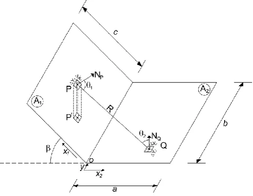
(2) where R is the distance between both differential elements dA1 and dA2; A1 and A2 are the faces of both surfaces; Φ1 and Φ2 are the angles between the normal vectors to both differential elements and the line between their centres (Fig. 2).
Page 359
Figure 2. Defining geometry for configuration factor
3.1.1. Orthogonal case
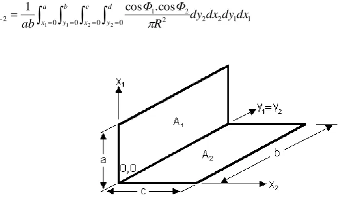
The cases, which find ready application with respect to building services, are two rectangular parallel surfaces and surfaces that are perpendicular to each other (See Fig. 3). The fundamental integral for two rectangular surfaces A1 with dimensions a × b and A2 with dimensions c × d is Equation (3),
a x
b y
c x
d
y
R
dy
dx
dy
dx
Φ
Φ
ab
F
0 0 0 0 2 2 2 1 1
2 1 2
1
1 1 2 2
cos
.
cos
1
(3)Figure 3. Two orthogonal surfaces with one common edge
For two perpendicular rectangular surfaces with a common edge b (Fig. 3), where
cos
Φ
1
x
2/
R
andR
x
Φ
/
cos
2
1 and 1 2 22 2 2
1
x
(
y
y
)
x
R
, the resulting integral is Eq. (4):
ax b y
c x
b
y
dy
dx
dy
dx
y
y
x
x
x
x
ab
F
0 0 0 0 2 2 2 2 1 1
2 1 2 2 2 1
2 1 2
1
1 1 2 2
(
)
1
Page 360
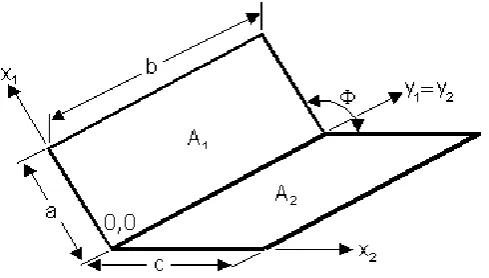
Figure 4. Two rectangular surfaces with one common edge and included angle of Φ
This generalised case, once again, has a number of applications such as solar energy reflected off ground and incident on a sloping roof, solar thermal water or air collectors or indeed photovoltaic modules. Note that for any given situation the ground reflected radiation may emanate from a conglomeration of surfaces of disparate reflectivities such as grass (ρ=0.24), tarmac (ρ=0.15), soil (ρ=0.12-0.25), other roof tops (0.13), pebbles (ρ=0.14-0.56) or water bodies (ρ=0.05-0.2).
The integration of Equation (2) for the case under discussion is rather involved. It does not lead to an exact solution, as was provided for the special case of Φ = 90o – see Equation (5). It rather leads to a partial, analytically integrable, one part, and the other part that is only numerically obtained.
If we apply Equation (3) to two rectangular surfaces A1 with dimensions a × b and A2 with dimensions c × b, with angle Φ between them (Fig. 5 and Fig. 6), then the resulting integral is Equation (6):
a
x b y
c x
b
y dy dxdydx
y y x
x x x
x x ab
F
0 0 0 0 2 2 2 2 1 1
2 1 2
1 2 2 2 1
2 2 1 2
1
1 1 2 2
) (
cos 2
sin 1
Page 361
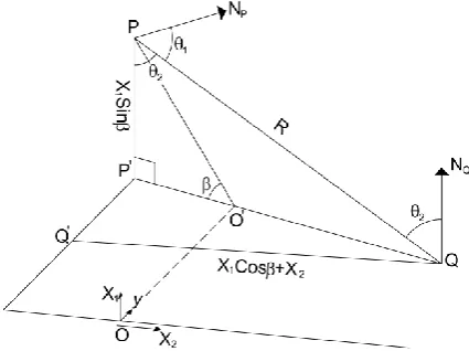
Figure 5. Projection of A1 and A2 surfaces on the X2/Y and X2/Z planes.
Figure 6. Detail of projection X2/Z plane
The solution of this integral is Equation (7). The last part of Equation (7) is unsolvable integral. This explains why a complete analytical solution of Equation (6) does not exist. The view factor F1-2 can be estimated partially analytically, partially numerically.
dz Φ z Φ z A Φ z Φ z Φ z B Φ D Φ A B D Φ A AD B Φ Φ C B C A B A B C C A A A B C C B B C B A Φ B Φ Φ A Φ A B A Φ B Φ B A B B A Φ Φ AB B Φ F B Φ Φ
0 2 2
1 2 2 1 2 2 1 1 1 1 1 2 cos 2 cos 2 2 2 2 2 2 2 2 2 2 1 2 1 2 2 2 2 1 sin 1 cos tan sin 1 cos tan sin 1 cos cos tan cos tan 2 2 sin sin 1 tan 1 tan 1 tan 1 ) 1 ( ) 1 ( ln ) 1 ( ) 1 ( ln 1 ) 1 )( 1 ( ln 1 sin 2 4 sin sin cos tan sin cos tan 2 sin 4 2 sin (7)
Page 362
j j i i
j i j i j i i j
y
y
Φ
x
x
x
x
Nb
Na
1 1 1 12 2 2
2
1 2 1 2
2
cos
(
)
.
.
(8)
where Δa = a / Na, Δb = b / Nb, Δc = c / Nc and Na, Nb, Nc are the numbers of intervals for the numeric integration in each dimension. The coordinates of each fragment’s center are: for surface i – xi=(i1–0.5)Δc; yi=(i2–0.5)Δb; for surface j – xj=(j1–0.5)Δa; yj=(j2–0.5)Δb. Such solution has one main significant advantage – it easily can be adapted for any disposition of both rectangular surfaces (Fig. 8), but also has two serious disadvantages – it gives an approximate result and to avoid this with large numbers of intervals, it needs a lot of computing time.
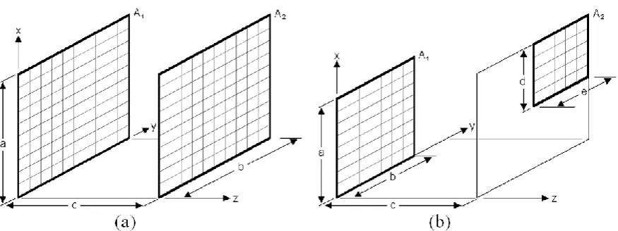
3.1.4. Derivation of a numerically integrable, general purpose VF: two parallel directly opposed rectangular surfaces Ai and Aj
For two parallel directly opposed rectangular surfaces (Fig. 7), Eq. (2) will have to be modified with these values of
2 2 1 2 2 1 2 2
1 ) ( ) ( )
(x x y y z z
R and cosΦ1cosΦ2c/R. The resulting integral for the estimation of VF1-2 is Eq. (9):
a x b y a x by dydx dydx
z z y y x x ab c F
0 0 0 0 2 2 2 2 1 1
2 1 2 2 1 2 2 1 2 2 1
1 1 2 2 ( ) ( ) ( )
1
(9)
Note that the configuration factor – solution of this integral, is Eq. (10), where X= a / c and Y= b / c:
1/2
Page 363
Figure 7. The reflecting and receiving surfaces are divided in two directions to receive a regular perpendicular grid: (a) both surfaces are identical and directly opposite; (b) two parallel surfaces –
generalized arrangement
If we consider both parallel and directly opposite rectangular surfaces Ai and Aj as composed of very many small rectangular areas, we could use numerical integration to obtain the same result with only a small loss of accuracy:
Naj Nb
j Na
i Nb
i i j i j i j
i
j
b
a
z
z
y
y
x
x
Nb
Na
c
F
1 1 1 1
2 2 2
2 2
1 2 1 2
(
)
(
)
(
)
1
.
.
(11) where c is distance between both surfaces, Δa = a / Na, Δb = b / Nb and Na, Nb are the numbers of intervals for the numerical integration in both dimensions.
4. PEDAGOGICAL EXERCISES
Equations (8) and (11) can now form the basis of numerically integrating codes to obtain view factors for the respective cases, i.e. inclined surfaces that share a common edge and parallel-opposed surfaces. The following two cases may be used for evolution of code architecture from simple-most and yet of low efficiency to highly-efficient but more complex. Those cases are:
4.1. Uniform grid
Page 364
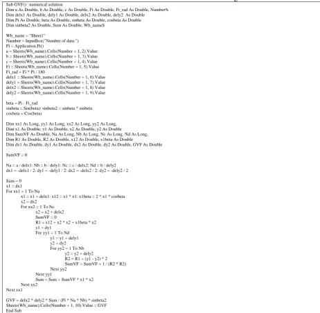
Table 1. VBA code for inclined surfaces: uniform grid
Sub GVF() ' numerical solution
Dim a As Double, b As Double, c As Double, Fi As Double, Fi_rad As Double, Number% Dim delx1 As Double, dely1 As Double, delx2 As Double, dely2 As Double
Dim Pi As Double, beta As Double, sinbeta As Double, cosbeta As Double Dim sinbeta2 As Double, Sum As Double, Wb_name$
Wb_name = "Sheet1"
Number = InputBox("Number of data:") Pi = Application.Pi()
a = Sheets(Wb_name).Cells(Number + 1, 2).Value b = Sheets(Wb_name).Cells(Number + 1, 3).Value c = Sheets(Wb_name).Cells(Number + 1, 4).Value Fi = Sheets(Wb_name).Cells(Number + 1, 5).Value Fi_rad = Fi * Pi / 180
delx1 = Sheets(Wb_name).Cells(Number + 1, 6).Value dely1 = Sheets(Wb_name).Cells(Number + 1, 7).Value delx2 = Sheets(Wb_name).Cells(Number + 1, 8).Value dely2 = Sheets(Wb_name).Cells(Number + 1, 9).Value beta = Pi - Fi_rad
sinbeta = Sin(beta): sinbeta2 = sinbeta * sinbeta cosbeta = Cos(beta)
Dim xx1 As Long, yy1 As Long, xx2 As Long, yy2 As Long, Dim x1 As Double, y1 As Double, x2 As Double, y2 As Double
Dim SumVF As Double, Na As Long, Nb As Long, Nc As Long, Nd As Long, Dim R1 As Double, R2 As Double, x12 As Double, x1beta As Double
Dim dx1 As Double, dy1 As Double, dx2 As Double, dy2 As Double, GVF As Double SumVF = 0
Na = a / delx1: Nb = b / dely1: Nc = c / delx2: Nd = b / dely2 dx1 = -delx1 / 2: dy1 = -dely1 / 2: dx2 = -delx2 / 2: dy2 = -dely2 / 2 Sum = 0
x1 = dx1 For xx1 = 1 To Na
x1 = x1 + delx1: x12 = x1 * x1: x1beta = 2 * x1 * cosbeta x2 = dx2
For xx2 = 1 To Nc x2 = x2 + delx2 SumVF = 0
R1 = x12 + x2 * x2 + x1beta * x2 y1 = dy1
For yy1 = 1 To Nd y1 = y1 + dely1 y2 = dy2 For yy2 = 1 To Nb
y2 = y2 + dely2 R2 = R1 + (y1 - y2) ^ 2 SumVF = SumVF + 1 / (R2 * R2) Next yy2
Next yy1
Sum = Sum + SumVF * x1 * x2 Next xx2
Next xx1
Page 365 4.2. Arithmetic Progression
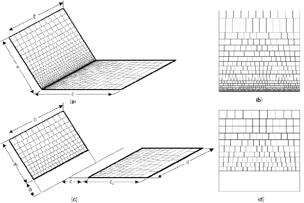
This case is applicable for inclined surfaces. A non-uniform grid in which the cell dimensions increase in an arithmetic progression as one moves from the common edge (Fig. 9). This development may be undertaken once the nature of influence of cells receding from the common edge is systematically studied. The shape of each cell is as close as possible to a square. This is especially important for the cells in the rows that are closer to the common line, because any other proportion of these cells generates significant errors in the result. The size of cell in first row of both surfaces is equal to the step in the arithmetic progression. The algorithm is the same for a composition of two surfaces with common edge and for a composition of non-intersecting rectangular surfaces that are inclined to each other. The number of square cells on the receiving surface as shown in Fig. 9a and b is Nreceiving_cells = (b/a).Na.(Na +1).(1+1/2+1/3+...+1/Na)/2, the number of square cells on the receiving surface as shown in Fig. 9c and d is Nreceiving_cells=(b/a2).Na.(Na +1).(1+1/2+1/3+...+1/Na)/2. The number of square cells on the emitting surface can be estimated by analogy. It may be shown that the total number of iterations is Nreceiving_cells.Nemitting_cells. Codes for this and other cases are provided at this website: https://www.dropbox.com/sh/8eehqf5szu1u68x/AAD4z7GFYkztzf-VgUqvHg7ea?dl=0
Figure 9. A non-uniform grid, where cell sizes increase in arithmetic progression, could be applied on: (a, b) two rectangular surfaces with one common edge; (c, d) two non-intersecting rectangular surfaces
that are inclined to each other
Some of the tutorial material that may now be developed for providing a taught module in radiation exchange is presented below:
a) Identify the practical engineering and architectural applications for radiation exchange for the configurations presented in Figs. 3, 4 and 7.
b) Consider Fig. 3. For a given parametric values of a=3, b=6 and c=6 units obtain the view factor F12 using Eq. 5. Note: you may obtain the solution using your calculator. You may then progress to using Microsoft-Excel worksheet, keying in the functions in a step-wise manner. In each case keep account of the time taken for your entire activity and the accuracy of the solution obtained. Note that the precise answer for this case is 0.292373.
c) Refer to Fig. 4. Repeat Exercise ‘b’ for the case of an inclination angle Φ=120o
.Note that the precise answer for this case is 0.129731.
Page 366
and easy going. Help is available in the form of well-written text, study guides, and training videos. An introduction to application of Excel in solving heat transfer problem takes 30 to 45 minutes of class time to demonstrate how to enter formulas into cells of Excel worksheet.
The advantage of using a spreadsheet-based computing environment such as Microsoft Excel is that the training times are of the order of, at most, a few hours to include finite element analysis (FEA) to obtain complex analysis such as those presented in the article.
A set of seven tutorial exercises were presented that will enable the pupils to gain a thorough understanding of not only the science of radiation exchange but also the use of a powerful computing medium such as Microsoft Excel-VBA to analyse complex engineering problems.
REFERENCES
ASHRAE Guide to Fundamentals (2013), American Society for Heating, Refrigeration and Air-conditioning Engineers, Atlanta, USA.
CIBSE Guide A (2015). Chartered Institution of Building Services Engineers, London, UK. Court MC (2004). The Impact of Using Excel Macros for Teaching Simulation Input and Output Analysis, International Journal of Engineering Education, 20 (6), pp. 966-973.
Karimi A (2008). AC 2008-1867: Use of spreadsheets solving heat conduction problems in fins. American Society for Engineering Education.
Liengme, B.V. (2009) A guide to Microsoft Excel 2007 for scientists and engineers, Academic Press, London, UK.
Muneer T., Kubie J. and Grassie T. (2003). Heat Transfer. A problem solving approach. Taylor & Francis Ltd, London, UK, New York, EEUU, pp. 388.