Sampling-standardized expansion and collapse of reef building
in the Phanerozoic
Wolfgang Kiessling
*
Museum fr Naturkunde der Humboldt-Universitt zu Berlin, Invalidenstraße 43, 10115 Berlin, Germany. E-mail: [email protected]
Introduction and background
Geologists have long suggested that the Phanerozoic re-cord of marine reefs fluctuated considerably through time but exactly how strong these fluctuations were is still a matter of debate. The published graphs of several authors suggest moderate fluctuations in reef abun-dance over the Phanerozoic (James 1983; Copper 1988; James & Bourque 1992; Hallock 1997), while other authors have depicted substantial variations, which increase with refinements of reef definitions (Wood 1993; Webb 1996; Kiessling et al. 1999, 2000; Kiess-ling 2002). Although there is more agreement on the timing of reef expansions and declines, the strati-graphic position and significance of reef booms are also poorly constrained. Resolving the issues of the temporal variability (= volatility) of reef growth and the position of reef booms and bursts is important for several reasons: First, identifying true peaks of reef growth can shed light on the global environmental con-ditions under which reefs tend to flourish. Second, the intensity of temporal fluctuations in reef abundance illuminates the sensitivity of reefs to extrinsic controls, be they environmental or biological. Third, insights can be gained into general processes of reef waxing and waning through time, because gradual increases and declines of reef abundance may suggest linear
relation-ships between control and effect, whereas sharp peaks and drops could indicate non-linear relationships or even self-organization.
Two major problems hinder the detection of biologi-cally meaningful patterns in reef production on geologi-cal time sgeologi-cales: Genuine variations in the preservation of sedimentary rocks and (economically driven) hetero-geneities in exploration intensity (Kiessling 2005a, 2006). Kiessling (2006) has tried to compensate for much of this bias and uncovered the probable pattern of changes in absolute reef abundance and volume through the Phanerozoic. His pattern of a maximum proliferation of reefs in the Silurian and Devonian and a steep decline thereafter, interrupted by short-term peaks, provides insights into absolute changes in reef production, but does not elucidate variations relative to changes in the fossil record. These relative changes, however, can be even more informative than absolute changes. Imagine for example, that reef abundance were determined merely (and linearly) by available shelf area and thus controlled by sea-level fluctuations and hypsography. Then we could use the reef record to trace ancient sea levels but a prefect correlation be-tween reef abundance and sea level would make it un-likely that any additional factors are relevant. Differ-ences between preserved reef abundance and overall sampling of the fossil record can reveal times when
ex-museum fu¨ r naturkunde
der Humboldt-Universita¨ t zu Berlin
Received 6 July 2007 Accepted 1 August 2007 Published 15 February 2008
Key Words
Reefs Phanerozoic fossil record sampling bias volatility
Abstract
pansions and collapses were due to other factors such as changes in paleoclimate or biological innovations.
These differences are the focus of this study. I com-pare a comprehensive database on Phanerozoic reefs (the PaleoReefs database) with another comprehensive database of marine invertebrate fossils (the Paleobiol-ogy Database) to find biologically meaningful depar-tures in reef production relative to the overall fossil re-cord.
Data and methods
This study utilizes two large databases: The PaleoReefs database (PARED) and the Paleobiology Database (PBDB). The structure and data inventory of both databases have either been discussed elsewhere (Kiessling & Flgel 2002) or are available online (http://paleodb.org). In brief, PARED compiles geological and paleontological information of Phanerozoic reef complexes and the PBDB hosts taxonomic collec-tion data of Phanerozoic protists, plants and animals. A reef in PARED is defined as a “laterally confined biogenic structure, devel-oped by the growth or activity of sessile benthic organisms and exhi-biting topographic relief and (inferred) rigidity” (Flgel & Kiessling 2002a). Although the information in both databases largely stems from the published literature, there are slightly different sampling strategies. In PARED virtually all data were collected by a single en-terer (W. Kiessling) who tried to get all the available information on fossil reefs, irrespective of age and geographic setting, that is, no stra-tigraphic or geographic foci were a priori defined. The PBDB in con-trast was compiled by a large suite of authorizers and enterers, with an often pronounced focus on particular time intervals. Although the time intervals that first suffered from less attention have later been filled with data to homogenize the time series, the sampling in PBDB probably represents a non-random fraction of the published literature. However, a random subset of the published literature (1%) was ex-tracted from GeoRef and analyzed in a project within the PBDB. Every hundredth accession number was obtained from GeoRef, which contained as keywords at least one of the major marine invertebrate phyla (Mollusca, Brachiopoda, Cnidaria, etc.). This 1% subset (down-loaded in summer 2003 by Michael Foote) contains 1175 references, 517 of which report original taxonomic collection data in peer-re-viewed publications. Roughly 60% of these references have been en-tered until now, with all geological periods being proportionally equally represented by references, that is, 60% of the useful refer-ences available for each period have been entered. Therefore, collec-tion counts in the 1% project should best reflect actual paleontologi-cal sampling intensity in the Phanerozoic. However, the fairly low number of references on which the collection counts are based (316) implies that individual references may contribute strongly to the esti-mate of sampling intensity. In other words, sampling peaks could be erroneously inferred when a few references report many collections from individual time intervals. This risk is much lower for the reef record and the total marine invertebrate record, which are based on 2573 and 4803 references, respectively. An additional sampling curve was thus created, which counts references instead of collections for the 1% data.
Other potential biases relate to the distribution of environmental settings and the distribution of geographic scales of collections in the PBDB. Data in PARED usually represent shallow marine carbonate environments and have a uniform geographic scale (Kiessling 2005b); whereas a variety of marine environments is present in the marine in-vertebrate data and an individual collection in the PBDB may repre-sent a hand sample, small collection, an individual outcrop or even a local area or basin. This would be a bias only if some time intervals bear unusual departures from the overall distributions. A cursory look
at the data suggests that there are no extreme outliers, except perhaps for an unusual concentration of “hand sample” data in the Cretaceous of the 1% project.
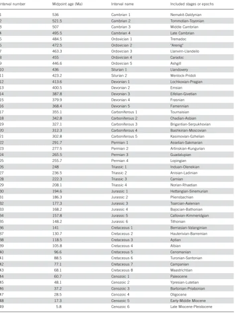
The stratigraphic resolution in both databases is variable, ranging from single ammonite zones to epochs. I apply here PBDB’s standard subdivision of the Phanerozoic, which separates 49 intervals of roughly equally duration (Table 1). All reef records and collections that could not confidently be assigned to one of these intervals were excluded from the analyses. The total counts of usable data as of 29 June 2007 are: 2972 reef sites, 40 417 marine invertebrate collec-tions, and 2151 collections in the 1% project. These values represent between 84% and 89% of the total counts in each dataset.
The reef record was broken down further to provide biologically more meaningful patterns. I limited the partitioning to two further cat-egories: The first subdivision considered only reefs dominated by metazoans and thus excluded microbial and algal reefs (metazoan reefs). The second subdivision was restricted to shallow-water reefs dominated by stony corals (tabulate, rugose or scleractinian corals) or hypercalcified sponges (archaeocyaths, stromatoporoids, chaetetids and pharetronids), which are not occurring in very high (> 45 degrees) paleolatitudes. The latter category is most similar to modern tropical coral reefs and therefore receives the most attention in the discussion. The discussion of ecological similarities between Paleozoic stromato-poroid-coral reefs and modern coral-algal reefs goes back and forth, usually focusing on the presence or absence of photosymbionts (Co-wen 1988; Wood 1993). Although there may be profound ecological differences among the coral-sponge reefs, a more refined definition would not permit a complete Phanerozoic time series to be created.
The analysis consists of three steps: I first describe the time series in terms of general pattern, autocorrelations, trends, position of peaks, and volatility. Trends are explored with correlation tests of abundance versus age. Volatility is assessed by the standard deviation of first differences. Although standard measures of volatility use proportional rather than absolute changes (Kiessling 2006), this approach is not feasible here, because some reef time series include null values. How-ever, the differences in scale need to be taken into account by calcu-lating the standard deviation of first differences of normalized values (proportional differences from the mean). The volatility of an abun-dance valueNis thus computed by:
VolatN¼stdððNt=NNtÞ ðNt1=NNtÞÞ:
In the second step, I apply statistical tests on the similarity of all curves to test the hypothesis that the reef record in PARED is actually related to the collection record in the PBDB. In the third step, I assess the standardized residuals (z-scores) of reef abundance regressed against the proxies of paleontological sampling. The standardization has the advantage of directly reporting values that can be used to as-sess the significance of outliers. I first use the raw counts because they are more intuitively understood, but the focus is on the pattern of first differences to circumvent the problem of autocorrelations. These sampling-standardized changes in reef abundance are then dis-cussed in detail for coral-sponge reefs. All analyses were performed under R 2.5.1.
Sampling patterns
Table 1.Definition of time intervals used for all analyses.
Interval number Midpoint age (Ma) Interval name Included stages or epochs
1 536 Cambrian 1 Nemakit-Daldynian
2 521.5 Cambrian 2 Tommotian-Toyonian
3 507 Cambrian 3 Middle Cambrian
4 495.5 Cambrian 4 Late Cambrian
5 484.5 Ordovician 1 Tremadoc
6 472.5 Ordovician 2 "Arenig"
7 463.3 Ordovician 3 Llanvirn-Llandeilo
8 455 Ordovician 4 Caradoc
9 446.6 Ordovician 5 Ashgill
10 436 Silurian 1 Llandovery
11 423.2 Silurian 2 Wenlock-Pridoli
12 413.6 Devonian 1 Lochkovian-Pragian
13 400.5 Devonian 2 Emsian
14 387.8 Devonian 3 Eifelian-Givetian
15 379.9 Devonian 4 Frasnian
16 368.4 Devonian 5 Famennian
17 355.1 Carboniferous 1 Tournaisian
18 342.8 Carboniferous 2 Chadian-Asbian
19 327.1 Carboniferous 3 Brigantian-Serpukhovian
20 312.3 Carboniferous 4 Bashkirian-Moscovian
21 302.8 Carboniferous 5 Kasimovian-Gzhelian
22 291.7 Permian 1 Asselian-Sakmarian
23 277.5 Permian 2 Artinskian-Kungurian
24 265.5 Permian 3 Guadalupian
25 255.7 Permian 4 Lopingian
26 248 Triassic 1 Induan-Olenekian
27 236.5 Triassic 2 Anisian-Ladinian
28 222.3 Triassic 3 Carnian
29 208.1 Triassic 4 Norian-Rhaetian
30 194.6 Jurassic 1 Hettangian-Sinemurian
31 186.3 Jurassic 2 Pliensbachian
32 177.3 Jurassic 3 Toarcian-Aalenian
33 168.2 Jurassic 4 Bajocian-Bathonian
34 157.8 Jurassic 5 Callovian-Kimmeridgian
35 148.2 Jurassic 6 Tithonian
36 141 Cretaceous 1 Berriasian-Valanginian
37 130.7 Cretaceous 2 Hauterivian-Barremian
38 118.5 Cretaceous 3 Aptian
39 105.8 Cretaceous 4 Albian
40 96.6 Cretaceous 5 Cenomanian
41 88.5 Cretaceous 6 Turonian-Santonian
42 77.1 Cretaceous 7 Campanian
43 68.1 Cretaceous 8 Maastrichtian
44 60.7 Cenozoic 1 Paleocene
45 48.1 Cenozoic 2 Ypresian-Lutetian
46 37.2 Cenozoic 3 Bartonian-Priabonian
47 28.5 Cenozoic 4 Oligocene
48 17.3 Cenozoic 5 Early-Middle Miocene
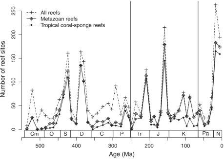
reefs” curve as well as with each other (Spearman-rank correlation, rS>0.89). The peaks in the three time ser-ies usually overlap, which is especially true for the ma-jor peaks in the Wenlock-Pridoli (Silurian 2), Middle Devonian and Frasnian (Devonian 3 and 4), Norian-Rhaetian (Triassic 4), Callovian-Kimmeridgian (Jurassic 5), and Neogene (Cenozoic 5 and 6). The major differ-ences among the curves are in the Cambro-Ordovician and the Carboniferous to Middle Triassic, when me-tazoan-dominated reefs were depleted relative to micro-bial and algal reefs. Another departure is between me-tazoan reefs and coral-sponge reefs for much of the Cretaceous, when rudists were important “reef ” builders (see Gili et al. 1995 for discussion). Although the Miocene represents a sampling peak in all time ser-ies, only the metazoan and coral-sponge reefs show sig-nificant Phanerozoic trends of better sampling in younger intervals (rS¼0.41, p¼0.004 and
rS¼ 0.32, p¼0.027, respectively). The volatility of reef abundance increases with constraints: The “all reefs” time series has the lowest volatility (1.11) and coral-sponge reefs the largest (1.43).
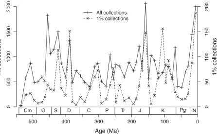
The time series of collection counts shares several attributes with the reef abundance curves (Fig. 2). Although sampling peaks are less pronounced, there are
distinct peaks in Silurian 2, Devonian 3, Jurassic 5 and the Neogene (Cenozoic 5 and 6). Autocorrelations are low and not significant for the collection counts. A sig-nificant relationship between sampling and age is only evident for the 1% collections (rS¼ 0.30, p¼0.04). This is surprising considering the exponential decay of sedimentary rocks (Gregor 1985) and their outcrop area (Raup 1976). For the “all collection” counts this poor match was somewhat expected because, as discussed under “data and methods”, the PBDB has deliberately tried to achieve a uniform number of collections from different time bins, rather than just letting the data fol-low the available material. This is also evident from the low volatility of the curve (0.63). However, the also weak correlation with the 1% collection counts sug-gests that paleontological sampling follows the avail-able rock record only weakly. The volatility of the 1% data (1.40) is similar to the coral-sponge reef data. Although the cross-correlation of first differences be-tween the two sampling curves is significant (rS¼0.43, p¼0.002), visual inspection of Fig. 2 shows that sampling peaks do not always match. As al-ready discussed under “data and methods” each of the two curves has its potential biases. Although the 1% curve may better reflect actual sampling intensity in
Age (Ma)
s
eti
s f
e
er
f
o
r
e
b
m
u
N
500
400
300
200
100
0
0
5
2
0
0
2
0
5
1
0
0
1
0
5
0
All reefs
Metazoan reefs
Tropical coral-sponge reefs
Cm
O
S
D
C
P
Tr
J
K
Pg
N
Figure 1.Time series of Phanerozoic reef sites per temporal interval of 49 units of approximately 11 myr duration (see Table 1).
the published literature than the total curve, some of the peaks in the former may be deceived by the un-usually strong contribution of just a few references. This appears to be true in the Cretaceous (most prominently in the Albian, Cretaceous 4) when sampling peaks in the 1% curve coincide with sampling lows in the total curve. To identify the potentially most problematic in-tervals, I have computed the number of collections per reference and interval for the 1% data. On average 5.9 collections were reported per reference (med-ian = 4.2) and the distribution is strongly right-skewed, which is expected when most references report only a few collections but a few references report many col-lections. The top three proportions are in Permian 4
(38.5 collection per reference), Jurassic 4 (13.1) and Cretaceous 4 (13.0). Counting references instead of col-lections probably reflects better the actual variations of sampling intensity (Fig. 3), but this approach is biased by low sample size. The reference curve has only a few distinct peaks in Devonian 3, Jurassic 5, Cretaceous 6 and the Neogene and a moderate volatility of 0.73.
Reef abundance versus sampling
There are significant cross-correlations between changes in reef abundance and changes in all individual proxies of sampling intensity (Table 2). This suggests that changes in reef abundance are partially controlled by changes in sampling intensity. Two general observa-tions from the correlation tests are noteworthy: (1) the correlations are weakest for all reefs and strongest for metazoan reefs; (2) the 1% collection data give the highest correlation coefficients. The highest correlation was observed between the curves of metazoan reefs and 1% collections, where 40% of the variance in reef abundance is explained by changes sampling intensity. Because autocorrelations are usually low, I have also tested the correlations between raw data. These correla-tions show the same basic results as the first differ-ences. None of the correlations indicate that the pattern of reef abundance is dominantly controlled by the pat-tern of sampling, which leaves the possibility of pro-cesses that are independent of sampling. However, the
Age (Ma)
s
n
oit
c
ell
o
c l
l
A
500 400 300 200 100 0
0
0
0
2
0
0
5
1
0
0
0
1
0
0
5
0
0
0
2
0
5
1
0
0
1
0
5
0
s
n
oit
c
ell
o
c
%
1
All collections 1% collections
Cm O S D C P Tr J K Pg N
Figure 2.Time series of collection counts in 49 Phanerozoic intervals. “All collections” refers to the total collections in the marine
invertebrate working group of the Paleobiology Database. “1% collections” indicates the number of collections in the 1% random selection of the published literature. Note the different scale of the two time series.
Age (Ma)
s
e
c
n
er
ef
er
f
o
r
e
b
m
u
N
500 400 300 200 100 0
5
3
0
3
5
2
0
2
5
1
0
1
5
0
Cm O S D C P Tr J K Pg N
Figure 3. Time series of entered reference counts in the 1%
correlations need to be taken into account to identify sampling-standardized reef abundance curves.
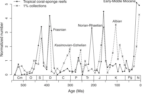
The logical next step is thus to look at differences between the sampling curves and the reef curves. A qualitative comparison can be done by visual inspection of the raw data (Fig. 4), but a quantitative tests needs to analyze residuals of linear regressions. In addition to analyzing all sampling proxies separately, I have per-formed multiple regressions of reef abundances versus all possible combinations of sampling proxies to find the combination of variables with the greatest explana-tory power. This “best match” was achieved for the combination of “1% collections” and “all collections” whose combined changes explain 50% of the variance in the changes of metazoan reef abundance (the “1%
references” proxy is uncorrelated in the multiple regres-sion analysis). The following sections discuss standar-dized residuals of reef abundance regressed against the best individual predictor (1% collections) and that best combination (= best match) of variables.
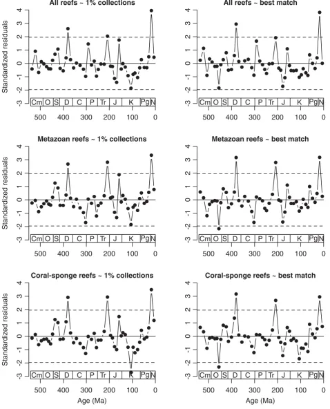
Although hampered by sometimes autocorrelated time series, the residuals of the raw data are more intui-tively understandable are thus reported first. The plots (Fig. 5) are surprisingly uniform in their basic patterns. There is agreement among all plots that most of the Phanerozoic reef record is neither unusually rich nor unusually depleted when viewed against the overall sampling of the fossil record. There is also agreement that there were at least three significant reef peaks rela-tive to sampling intensity: One in the Frasnian
(Devo-Table 2.Cross-correlations of changes in reef abundance and changes in proxies of sampling intensity.
All collections 1% collections 1% references
All reefs rS¼0.31, p¼0.030 rS¼0.53, p<0.001 rS¼0.42, p¼0.003 Metazoan reefs rS¼0.41, p¼0.004 rS¼0.63, p<0.001 rS¼0.56, p<0.001 Coral-sponge reefs rS¼0.37, p¼0.010 rS¼0.58, p<0.001 rS¼0.48, p<0.001
Age (Ma)
r
e
b
m
u
n
d
e
zil
a
mr
o
N
500
400
300
200
100
0
5
4
3
2
1
0
Tropical coral-sponge reefs
1% collections
Norian-Rhaetian
Frasnian
Kasimovian-Gzhelian
Albian
Early-Middle Miocene
Cm
O
S
D
C
P
Tr
J
K
Pg
N
Figure 4. Normalized (individual values divided by mean values) counts of coral-sponge reefs and collections per interval. This
All reefs ~ 1% collections
sl
a
u
di
s
er
d
e
zi
dr
a
d
n
at
S
500 400 300 200 100 0
4
3
2
1
0
1-
2-3- Cm O S D C P Tr J K Pg N
Metazoan reefs ~ 1% collections
sl
a
u
di
s
er
d
e
zi
dr
a
d
n
at
S
500 400 300 200 100 0
4
3
2
1
0
1-
2-3- Cm O S D C P Tr J K Pg N
Coral-sponge reefs ~ 1% collections
Age (Ma)
sl
a
u
di
s
er
d
e
zi
dr
a
d
n
at
S
500 400 300 200 100 0
4
3
2
1
0
1-
2-3- Cm O S D C P Tr J K Pg N
All reefs ~ best match
500 400 300 200 100 0
4
3
2
1
0
1-
2-3- Cm O S D C P Tr J K Pg N
Metazoan reefs ~ best match
500 400 300 200 100 0
4
3
2
1
0
1-
2-3- Cm O S D C P Tr J K Pg N
Coral-sponge reefs ~ best match
Age (Ma)
500 400 300 200 100 0
4
3
2
1
0
1-
2-3- Cm O S D C P Tr J K Pg N
Figure 5.Standardized residuals from the regression of reef counts (Fig. 1) against proxies of sampling intensity of Phanerozoic
nian 4), one in the Norian-Rhaetian (Triassic 4), and one in the Early to Middle Miocene (Cenozoic 5). It is further interesting that there were very few significant depressions in reef growth relative to sampling and that these depressions were either in the Cretaceous (Albian, Fig. 5 left column) or Ordovician (Caradoc, Fig. 5 right column) rather than in the aftermath of one of the big Phanerozoic mass extinctions, which are notorious for their poor or absent reef record (Flgel & Kiessling 2002b).
Is the volatility of sampling-standardized reef build-ing lower than in the raw data? To address this ques-tion, I have made the raw residual values positive by adding the absolute value of the minimum residual to all values. The volatilities, calculated according to equation (1), are indeed substantially lower for all standardized curves than for the raw curves. Surpris-ingly the curves, which originally showed the strongest fluctuations, are most affected: the volatility of the cor-al-sponge reef curve drops from 1.43 in the raw data to 0.47 or 0.56 (1% collections and best match, spectively) in the sampling-standardized curves, a re-duction of some 65%. The volatilities in the other curves also drop considerably (30–40%). This suggests that the noisiness of the Phanerozoic reef record is partially attributed to heterogeneities in the overall fos-sil record.
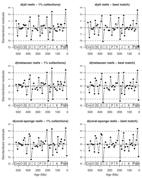
The analysis of first differences allows the detection of unusual changes in reef abundance relative to changes in sampling. This approach takes care of the autocorrelations observed in some time series of reef abundance (see “sampling patterns”) and is thus statis-tically more rigorous. The standardized residuals of the regressions (Fig. 6) indicate a more balanced pattern of significant rises and drops in reef abundance than the previous analysis. Three prominent increases of reef abundance relative to changes in sampling (Triassic 4, Jurassic 5, and Cenozoic 5) are mirrored by three or four substantial declines (Devonian 5, Jurassic 1, Ceno-zoic 6, and Jurassic 6 for the 1% collections). The pro-nounced negative excursions usually follow strong positive excursions. As in the analyses of raw data, the Big Five mass extinction events (Raup & Sepkoski 1982) are not pronounced in the sampling-standardized patterns of changes in reef abundance and there gener-ally is a poor match between relative declines in reef abundance and the reported intensity of mass extinc-tions (Sepkoski 1996; Foote 2003). Just two mass extinctions are matched by significant reef declines: the Frasnian-Famennian crisis and the Triassic-Jurassic mass extinction. Even the Permian-Triassic boundary exhibits only a very minor drop of reef abundance after controlling for sampling. This does not necessarily imply that all the apparent reef crises reported earlier (Flgel & Kiessling 2002b) are biased by incomplete sampling. Sampling and reef abundance may be affected by the same underlying processes such as sea-level change and plate tectonic regimes (Peters 2005, 2006).
Discussion of a sampling-standardized
reef curve
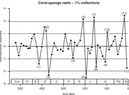
A closer look at the residuals of the regressions be-tween first differences is worthwhile because these graphs can be easily misread. In addition, the smaller (absolute z-scores of greater than 1) standardized resi-duals deserve at least some attention because they may hint to meaningful processes. Although all curves de-picted in Figs 5 and 6 show some interesting features, I limit the discussion to just one curve: the residuals of changes in tropical coral-sponge reef abundance and changes in collection counts of the 1% project (lower left-hand graph in Fig. 6, Fig. 7). I use tropical coral-sponge reefs because they are the biologically most uniform subset of PARED, which can be traced across the entire Phanerozoic and because the stability of Ho-locene tropical coral reefs is a major concern in global change biology (Pandolfi et al. 2003; Bellwood et al. 2004; Montaggioni 2005; Pandolfi & Jackson 2006). I compare changes of coral-sponge reefs with changes in the 1% collection data because these show the greatest individual cross-correlations among the proxies for sampling intensity. Although the “best match” combina-tion of variables is even better correlated with reef abundance, it is just easier to discuss a single variable and the “all collections” data in the best match are un-likely to truly follow the quality of the fossil record.
Per-mian periods exhibit modest fluctuations and even the end-Permian mass extinction did not result in a reef de-cline that could not be explained by changes in sam-pling (Fig. 7, number 4). This is not to say that there was no reef crisis at the Permian-Triassic boundary.
The ecological crisis of reefs is well documented (Weid-lich et al. 2003) and until recently no metazoan reefs were reported from the entire Early Triassic (Pruss et al. 2007). In terms of the decline in reef abundance the Early Triassic drop is just too well matched by a d(all reefs ~ 1% collections)
sl
a
u
di
s
er
d
e
zi
dr
a
d
n
at
S
500 400 300 200 100 0
3
2
1
0
1-
2-3- Cm O S D C P Tr J K Pg N
d(metazoan reefs ~ 1% collections)
sl
a
u
di
s
er
d
e
zi
dr
a
d
n
at
S
500 400 300 200 100 0
3
2
1
0
1-
2-3- Cm O S D C P Tr J K Pg N
d(coral-sponge reefs ~ 1% collections)
Age (Ma)
sl
a
u
di
s
er
d
e
zi
dr
a
d
n
at
S
500 400 300 200 100 0
3
2
1
0
1-
2-3- Cm O S D C P Tr J K Pg N
d(all reefs ~ best match)
500 400 300 200 100 0
3
2
1
0
1-
2-3- Cm O S D C P Tr J K Pg N
d(metazoan reefs ~ best match)
500 400 300 200 100 0
3
2
1
0
1-
2-3- Cm O S D C P Tr J K Pg N
d(coral-sponge reefs ~ best match)
Age (Ma)
500 400 300 200 100 0
3
2
1
0
1-
2-3- Cm O S D C P Tr J K Pg N
Figure 6.Standardized residuals from the regression of changes in reef counts against changes in proxies of sampling intensity of
similar drop in sampling to suspect biologically mean-ingful patterns from the abundance data alone.
The first significant rise in sampling-standardized reef abundance is evident in the Norian-Rhaetian inter-val and was followed by an also significant drop in the Hettangian-Sinemurian (Fig. 7, numbers 5–6). This pat-tern suggests that both the Norian-Rhaetian reef expan-sion and the Early Jurassic collapse have causes that would not affect sampling levels. Changes in nutrient regimes are held responsible for the former (Flgel 2002) and abrupt temperature rises for the latter (Mar-zoli et al. 2004; Kiessling & Aberhan 2007). The sig-nificant Callovian-Kimmeridgian rise of reef abundance (Fig. 7 number 7) comes as a surprise, because both coral-sponge reefs and sampling increase substantially in this interval (Figs 1, 2). The expansion of reefs, how-ever, is proportionally much larger than the increase in sampling, so that the standardized residual is the sec-ond largest in the entire Phanerozoic. A suite of cli-matic, oceanographic and biological changes is cur-rently discussed to explain the dramatic Late Jurassic (especially late Oxfordian-Kimmeridgian) reef boom (Leinfelder et al. 2002; Cecca et al. 2005). An explana-tion for the subsequent Tithonian decline (Fig. 7, num-ber 8) cannot be offered. Flgel and Kiessling (2002) noted a third order reef decline but found the most dra-matic collapse across the Jurassic-Cretaceous boundary, when the sampling standardized data show no deviation at all. The decline of coral reefs in the late Early Cre-taceous and the Cenomanian spike (Fig. 7, numbers 9–
10) should be interpreted with care, because here the results vary most strongly among proxies of sampling intensity. The agreement in the Cenozoic, however, sug-gests that the Early Neogene reef expansion (Fig. 7, number 11) is significant and a biological reality. This proliferation in spite of long-term global cooling (superimposing the mid-Miocene climatic optimum) can perhaps be explained by a relative increase in
low-nutrient habitat area, due to a reduction of equatorial upwelling (Perrin & Kiessling in press). The dramatic drop in the Late Miocene to Pleistocene was not ex-pected from the raw data, which suggest stability (Fig. 1). A late Miocene-Pliocene reef reduction has been previously suggested (Veron 1995) but attributed to a loss of habitat area owing to glacio-eustatic regres-sions, which should affect all marine life. Further cli-matic cooling could be responsible but I should empha-size a potential bias in PARED here. The reef data for the Late Miocene and Pliocene are fairly complete, but Pleistocene reefs were only recently entered into PARED and sampling is still incomplete. There are, however, many Pleistocene records in the 1% collection data (51 of 187 in Cenozoic 6), which artificially raises sampling estimates relative to reef counts.
Implications
We have seen that a substantial part of the changes in reef abundance can be explained by changes in paleon-tological sampling. None of our available proxies for sampling is perfect, but the concordance of the results among the three proxies studied herein suggests that the data are sufficiently robust to reach solid conclu-sions.
Sampling itself is controlled by a variety of factors, among them geologic (weathering, burial, diagenesis, metamorphosis, subduction), geomorphologic and cli-matic (accessible outcrop area), socioeconomic, physi-cal (ancient sea level, tectonics) and biological (changes in skeletal mineralogy, productivity). Only the latter two factors have some biological bearing: Sea lev-el and hypsography control habitat area that is known to have a significant influence on both diversity and abundance of organisms in general and reefs in particu-lar (Bellwood & Hughes 2001; Kiessling 2005a). Sea-level changes and tectonic factors that lead to the for-mation and destruction of marine habitats are currently discussed as the “common cause” scenario, which would affect sampling regimes, biodiversity and ecosys-tems simultaneously (Peters 2005, 2006). Evolutionary or ecological changes influencing the durability of shells or productivity are also of major interest in pa-leobiology (Martin 1995, 1996; Kershaw & Brunton 1999; Kidwell 2005). These factors are sacrificed when departures between sampling and the fossil record of an ecosystem are analyzed. The parallel waxing and waning of paleontological sampling and preserved reef abundance may be real and causally related, thus not strictly representing a bias. However, with the standar-dization for sampling one can approach factors that are otherwise hidden.
What conclusions can be drawn from the residuals and are they in agreement with our current understand-ing of reef development? I think the most interestunderstand-ing aspect of my results is the observation of substantial reef declines often following substantial expansions
Coral-sponge reefs ~ 1% collections
Age (Ma)
sl
a
u
di
s
er
d
e
zi
dr
a
d
n
at
S
500 400 300 200 100 0
3
2
1
0
1-
2-
3-(1) (2)
(3)
(4) (5)
(6) (7)
(8) (9)
(10) (11)
(12)
Cm O S D C P Tr J K Pg N
Figure 7. Standardized residuals from the regression of
(Late Devonian, Triassic-Jurassic boundary, Late Juras-sic, Neogene), which occur under very different environ-mental conditions. Although all individual reef booms and bursts can perhaps also be explained by specific en-vironmental and biological changes (see previous sec-tion), the big picture suggests more general principles that might be driven by intrinsic dynamics rather than en-vironmental change. This phenomenon, known as self-organized criticality, is a property of many dynamical systems that have a critical point as an attractor and are scale-invariant (Bak et al. 1987; Sol et al. 2002). In ecology, self-criticality is often inferred for complex eco-systems (Sol et al. 2002) and has also been suggested for carbonate sedimentation (Drummond & Dugan 1999). It would thus seem reasonable that complex car-bonate ecosystems such as reefs should exhibit proper-ties of self-organized criticality. If self-organization is ac-tually present in Phanerozoic reef building (further tests are clearly required), then the paradigm of reefs as pas-sive tracers of global change should be revisited.
Conclusions
The waxing and waning of Phanerozoic reefs is mostly in concord with the increase and decrease of paleontologi-cal sampling. Controlling for sampling greatly reduces the volatility in reef abundance and leaves only a few prominent intervals of reef expansion and subsequent de-cline. The standardization may overcompensate for bias because reef abundance and sampling can be causally re-lated through large-scale variations of sea-level, oceano-graphy or plate tectonic regimes. However, sampling standardization opens new opportunities for detecting signals in reef building that are not sampling-driven. The substantial fluctuations in sampling-standardized reef abundance thus demand specific attention. The typical pattern of substantial changes in reef abundance appears to be rapid expansions followed by collapse. If collapse is a consequence of expansion, then the focus of future research should be on the causes of extensive reef expan-sions such as those seen in the Middle Devonian-Fras-nian, Late Triassic, Late Jurassic and early Neogene.
Acknowledgements
The idea for this paper stems from a research visit to the Santa Fe Institute. I am grateful to Doug Erwin for inviting me there and to the Santa Fe Institute for logistic and financial support. Michael Foote and Lucien Montaggioni provided constructive and insightful reviews. I thank Uta Merkel for diligently entering data into the Paleobiology Database. Martin Aberhan and Loic Villier contributed substantially to the 1% project. The study was supported by the VolkswagenStif-tung. This is Paleobiology Database publication #66.
References
Algeo, T. J. & Scheckler, S. E. 1998. Terrestrial-marine teleconnec-tions in the Devonian – Links between the evolution of land plants, weathering processes, and marine anoxic events. –
Philo-sophical Transactions of the Royal Society of London Series B–
Biological Sciences 353: 113–128.
Bak, P., Tang, C. & Wiesenfeld, K. 1987. Self-organized criticality: An explanation of the 1/f noise. – Physical Review Letters 59: 381–384.
Bellwood, D. R. & Hughes, T. P. 2001. Regional-scale assembly rules and biodiversity of coral reefs.–Science 292: 1532–1535. Bellwood, D. R., Hughes, T. P., Folke, C. & Nystrm, M. 2004.
Con-fronting the coral reef crisis.–Nature 429: 827–833.
Cecca, F., Martin Garin, B., Marchand, D., Lathuiliere, B. & Bartolini, A. 2005. Paleoclimatic control of biogeographic and sedimentary events in Tethyan and peri-Tethyan areas during the Oxfordian (Late Jurassic). – Palaeogeography, Palaeoclimatology, Palaeoe-cology 222: 10–32.
Copper, P. 1988. Ecological succession in Phanerozoic reef ecosys-tems: is it real?–Palaios 3: 136–152.
Cowen, R. 1988. The role of algal symbiosis in reefs through time. –
Palaios 3: 221–227.
Drummond, C. N. & Dugan, P. J. 1999. Self-organizing models of shallow-water carbonate accumulation. – Journal of Sedimentary Research 69: 939–946.
Flgel, E. 2002. Triassic reef patterns.InKiessling, W., Flgel, E. & Golonka, J. (eds). Phanerozoic Reef Patterns: 391–463, SEPM Special Publication 72, Tulsa.
Flgel, E. & Kiessling, W. 2002a. A new look at ancient reefs. In
Kiessling, W., Flgel, E. & Golonka, J. (eds). Phanerozoic Reef Patterns. SEPM Special Publication 72, Tulsa: pp. 3–10. Flgel, E. & Kiessling, W. 2002b. Patterns of Phanerozoic reef crises.
InKiessling, W., Flgel, E. & Golonka, J. (eds). SEPM Special Publication 72, Tulsa: pp. 691–733
Foote, M. 2001. Inferring temporal patterns of preservation, origina-tion, and extinction from taxonomic survivorship analysis. – Pa-leobiology 27: 602–630.
Foote, M. 2003. Origination and extinction through the Phanerozoic: a new approach.–Journal of Geology 111: 125–148.
Gili, E., Masse, J. P. & Skelton, P. W. 1995. Rudists as gregarious sediment dwellers, not reef builders, on Cretaceous carbonate platforms. – Palaeogeography, Palaeoclimatology, Palaeoecology 118: 245–267.
Gregor, C. B. 1985. The mass-age distribution of Phanerozoic sedi-ments.In Snelling, N. J. (ed.). The Chronology of the Geologic Record. Geological Society of America, Memoir 10, Boulder: pp. 284–289.
Hallock, P. 1997. Reefs and reef limestones in earth history.In Birke-land, C. (ed.). Life and Death of Coral Reefs. Chapman & Hall, New York: pp. 13–42.
James, N.P. 1983. Reef environment.InScholle, P. A., Bebout, D. G. & Moore, C. H. (eds). Carbonate Depositional environments AAPG Memoir 33, Tulsa: pp. 345–440.
James, N. P. & Bourque, P.-A. 1992. Reefs and mounds.InWalker, R. G. & James, N. P. (eds). Facies Models: Response to Sea Level Change. Geological Association of Canada, St. John’s: pp. 323–347. Kershaw, S. & Brunton, F. R. 1999. Palaeozoic stromatoporoid
taph-onomy: ecologic and environmental significance.– Palaeogeogra-phy, Palaeoclimatology, Palaeoecology 149: 313–328.
Kidwell, S. M. 2005. Shell composition has no net impact on large-scale evolutionary patterns in mollusks.–Science 307: 914–917. Kiessling, W. 2002. Secular variations in the Phanerozoic reef ecosys-tem.InKiessling, W., Flgel, E. & Golonka, J. (eds). Phanerozoic Reef Patterns. SEPM Special Publication 72, Tulsa: pp. 625–690. Kiessling, W. 2005a. Habitat effects and sampling bias on
Phanero-zoic reef distribution.–Facies 51: 27–35.
Kiessling, W. 2005b. Long-term relationships between ecological sta-bility and biodiversity in Phanerozoic reefs. –Nature 433: 410–
413.
Kiessling, W. 2006. Towards an unbiased estimate of fluctuations in reef abundance and volume during the Phanerozoic. – Biogeo-sciences 3: 15–27.
Kiessling, W. & Flgel, E. 2002. Paleoreefs–a database on Phanerozoic reefs.InKiessling, W., Flgel, E. & Golonka, J. (eds). Phanerozoic Reef Patterns. SEPM Special Publication 72, Tulsa: pp. 77–92. Kiessling, W., Flgel, E. & Golonka, J. 1999. Paleoreef maps:
Evalua-tion of a comprehensive database on Phanerozoic reefs. –AAPG Bulletin 83: 1552–1587.
Kiessling, W., Flgel, E. & Golonka, J. 2000. Fluctuations in the car-bonate production of Phanerozoic reefs. InInsalaco, E., Skelton, P. W. & Palmer, T. J. (eds). Carbonate Platform Systems: compo-nents and interactions. Geological Society Special Publication 178, London: pp. 191–215.
Leinfelder, R. R., Schmid, D. U., Nose, M. & Werner, W. 2002. Juras-sic reef patterns –the expression of a changing globe.In Kiess-ling, W., Flgel, E. & Golonka, J. (eds). Phanerozoic Reef Pat-terns. SEPM Special Publication 72, Tulsa: pp. 465–520. Martin, R. E. 1995. Cyclic and secular variation in microfossil
biomi-neralization: clues to the biogeochemical evolution of Phanerozoic oceans.–Global and Planetary Change 11: 1–23.
Martin, R. E. 1996. Secular increase in nutrient levels through the Phanerozoic: implications for productivity, biomass, and diversity of the marine biosphere.–Palaios 11: 209–219.
Marzoli, A., Bertrand, H., Knight, K. B., Cirilli, S., Buratti, N., Vra-ti, C., Nomade, S., Renne, P. R., Youbi, N., Martini, R., Allen-bach, K., Neuwerth, R., Rapaille, C., Zaninetti, L. & Bellieni, G. 2004. Synchrony of the Central Atlantic magmatic province and the Triassic-Jurassic boundary climatic and biotic crisis. – Geol-ogy 32: 973–976.
Montaggioni, L. F. 2005. History of Indo-Pacific coral reef systems since the last glaciation: Development patterns and controlling factors.–Earth-Science Reviews 71: 1–75.
Pandolfi, J. M., Bradbury, R. H., Sala, E., Hughes, T. P., Bjorndal, K. A., Cooke, R. G., McArdle, D., McClenachan, L., Newman, M. J. H., Paredes, G., Warner, R. R. & Jackson, J. B. C. 2003. Global trajectories of the long-term decline of coral reef ecosystems. –
Science 301: 955–958.
Pandolfi, J. M. & Jackson, J. B. C. 2006. Ecological persistence inter-rupted in Caribbean coral reefs. –Ecology Letters 9: 818–826. Perrin, C. & Kiessling, W. in press. Latitudinal trends in Cenozoic
reef patterns and their relationship to climate.–IAS Special Pub-lications.
Peterhnsel, A. & Pratt, B. R. 2001. Nutrient-triggered bioerosion on a giant carbonate platform masking the postextinction Famennian benthic community.–Geology 29: 1079–1082.
Peters, S. E. 2005. Geologic constraints on the macroevolutionary his-tory of marine animals. – Proceedings of the National Academy of Science USA 102: 12326–12331.
Peters, S. E. 2006. Genus extinction, origination, and the durations of sedimentary hiatuses.–Paleobiology 32: 387–407.
Pruss, S. B., Payne, J. L. & Bottjer, D. J. 2007. Placunopsis bioherms: the first metazoan buildups following the end-Permian mass ex-tinction.–Palaios 22: 17–23.
Raup, D. M. 1976. Species diversity in the Phanerozoic: an interpreta-tion.–Paleobiology 2: 289–297.
Raup, D. M. & Sepkoski, J. J., Jr. 1982. Mass extinctions in the mar-ine fossil record.–Science 215: 1501–1503.
Ronov, A. B. 1994. Phanerozoic transgressions and regressions on the continents: a quantitative approach based on areas flooded by the sea and areas of marine and continental deposition. – American Journal of Science 294: 777–801.
Sepkoski, J. J., Jr. 1996. Patterns of Phanerozoic extinction: a perspec-tive from global data bases. In Walliser, O. H. (ed.). Global Events and Event Stratigraphy in the Phanerozoic. Springer, Ber-lin: pp. 35–51.
Sol, R. V., Alonso, D. & McKane, A. 2002. Self-organized instability in complex ecosystems.–Philosophical Transactions of the Royal Society of London Series B-Biological Sciences 357: 667–681. Veron, J. E. M. 1995. Corals in space and time. Cornell Press, Ithaca. Webb, G. E. 1996. Was Phanerozoic reef history controlled by the
distribution of non-enzymatically secreted reef carbonates (micro-bial carbonate and biologically induced cement)? – Sedimentol-ogy 43: 947–971.
Weidlich, O., Kiessling, W. & Flgel, E. 2003. The Permian-Triassic boundary interval as a model for forcing marine ecosystem collapse by long-term atmospheric oxygen drop.–Geology 31: 961–964. Wood, R. 1993. Nutrients, predation and the history of reef-building.
Palaios 8: 526–543.