OPTIMIZATION OF CONSECUTIVE SIGNALIZED INTERSECTIONS BASED ON COMBINED ALGORITHMS – COMPARING RESULTS WITH MICROSIMULATION

OPTIMIZATION OF CONSECUTIVE SIGNALIZED INTERSECTIONS

BASED ON COMBINED ALGORITHMS – COMPARING RESULTS

WITH MICROSIMULATION

Shahriar Afandizadeh Zargari1_{, Atousa Tajaddini}2_{, Mohammadreza Khalilzadeh}31

1 _{Iran University of Science and Technology, Department of Civil Engineering, Tehran, Iran}

2, 3 _{Islamic Azad University, South Tehran Branch, Tehran, Iran}

Received 14 August 2015; accepted 26 October 2015

Abstract: The primary objective of this research is to optimize signal timing in consecutive signalized intersections. In this paper, the combination of genetic programming (GP) with genetic algorithms (GA) and neural network (NN) with genetic algorithm (GA) were used and compared in order to optimize signal timing in consecutive signalized intersections. First, genetic programming and neural network were constructed from existing signal timing data to predict the delay of intersections. Then genetic algorithm was applied to optimize these predictive networks (GP and NN). The results and comparisons of timing process and error percentage showed that neural network is more efficient than genetic programming. However, the ability of genetic programming in producing formula is a specific characteristic which makes it more applicable than neural network. Finally, for validating the results, Aimsun and Synchro micro simulation software were used, and accuracy of our models was approved.

Keywords: signal timing, signalized intersections, optimization, neural network, genetic algorithm, genetic programming.

1. Introduction

Increase in urbanization and creation of traffic density can result in emergent need for creating transportation system with maximum efficiency. Over the past years, traffic control has been considered as a basic problem in many cities especially metropolitans. Applying traditional solutions such as increasing infrastructures cannot be a suitable and desirable solution for meeting current traffic problems (Girianna and Benekohal, 2002). One of the main effective factors in urban traffic is signalized intersection. Increase in capacity and decrease in delay in these intersections

applied under conditions of under saturated. In addition to mathematical models, many other models have been also presented based on simulation. The basic problem with these models is that they have no analytical basis and can use try and error for obtaining a suitable scheduling pattern (Hajbabaie et al., 2011; Dell’Orco et al., 2013). Such method has two main problems as follows: on one hand, achieving suitable answer is depended on engineering judgment and skill of the designer and there is no trust for being the best answer; on the other hand, the methods can’t be applied for automated controlling systems.

Meta-heuristic methods such as genetic algorithm and neural networks, genetic programming or intelligent learning methods such as approximate dynamic planning can be significantly effective as an exact traffic simulation instrument for purpose of determining optimized scheduling of traffic signs in transportation networks (Alodat and Al-Odat, 2013; Zang et al., 2012). Genetic Programming (GP) is a branch of genetic algorithm. The main difference between genetic programming and genetic algorithm is presenting solution method in GP. The system is one of the newest and most applicable systems with evolutional processing performance (Konig, 2014). If it is possible for solving problem to use different formulations and equations, GP is in fact a system for creating and developing a solution for the problem. In GP, hundreds or thousands processing programs or formula would be produced genetically (Searson, 2009; Searson et al., 2010). The production would be conducted using Darwin’s principles in the theory of Survival and evolution and with genetic combinational operators for intercross of formulas. Hence, GP is able to solve

complicated problems using Method of Growth of Populations based on Darwinian Evolution and Mendelian genetics. Genetic algorithm is an intelligent search method, which has the ability to find an optimized answer among limited number of answers through generation.

2. Literature Review

evolution algorithms were identified as optimization methods (Searson, 2009). By 1990, GP has been applicable mostly for simple problems because of its complicated calculation structure. Recently, GP has achieved brilliant and modern results in different research fields such as quantum calculations, electronic designing, and computer games classification and so on (Searson et al., 2010). Chang et al. (2010) proposed an optimization policy which was suitable for oversaturated intersections. Their method increased the efficiency of system through queue management. They tested their model on one over-saturated arterial with two intersections. The result showed this model increased the capacity of intersection and decreased average delay up to 22 percent (Chang et al., 2010).

3. Methodology

Based on HCM regulation, geometric status, traffic conditions and scheduling type of traffic signals can be the most effective factors in performance of traffic signals. In this regard, one can name basic parameters in phasing and scheduling traffic signs as follows: cycle length, green time, yellow time that is also known as changing time and also red time that is the time allowing the intersection to be discharged completely and type of phasing and sequence of phases (Highway Capacity Manual, 2000). Phasing variables are in form of determining simultaneous movements, sequence and their implementation. Right turn movement would be conducted usually with direct movement; although left turn movement can be predicted in form of protected, unprotected and a combination of the two modes.

At the first step, it would be necessary to

zone, number of lanes, average lane width and slope) and then, traffic conditions (including density of vehicles in each approach and finally origin-destination matrix in peak hour) in the network should be estimated. Finally, conditions of traffic signal should be determined at the current situation on peak hours (including cycle length, green time, the time between two greens, yellow time in addition to all red time and schedule of fixed and changing mode of signals). The network at the current situation would be modeled in Synchro Software and average delay would be obtained under such conditions.

study, would be produced in this layer and would be then compared to desired outputs. Propagation-Backward algorithm can arrange hidden layers through propagating output error in layered form to the backward and through regulating weights in each layer. Hence in a backward network, hidden layers can form main core of calculations and these layers can receive inputs from input layer using neurons and then, they produce amount of output in output layer. Each intersection would be scheduled separately and would be investigated under different schedules of whole network and delay can be estimated through this. Following, all collected data in previous steps would be analyzed using genetic programming with Multigene Symbolic Regression (MSR) and delay would be estimated through this. In genetic programming, there is no need for effective data because of nature of the system and using evolution theory. In fact, regression method of the system is in such manner that it uses some data during the analysis that create minimum error in estimations. As a result, using more data can cause empowerment of the schedule and minimization of errors.

In Multigene Symbolic Regression for input data, the primary population would be created using genetic programming, in which each individual includes several trees that their numbers can be determined. Then, minimum square of errors method would be applied for purpose of determining weight of each tree and fixed value in each formula. Afterwards, error level of each equation would be determined using competency function and the new population would be produced using the mentioned operators. The algorithm goes ahead in iterated mode based on the mentioned process. Final conditions and exiting from algorithm cycle is achieving

determined number of population or the desired error level. In fact, in each cycle of population production, the best formulation with the lowest error can be considered as the solution for the problem. Manner of performance of genetic programming (GP) and neural network (NN) is as follows: firstly, the network would be trained by 70% of collected data from intersections with different schedules applied on them and then it would be validated with the remained 30% of the data. The data are same different durations of the cycle, along with different phasing modes, which can be obtained from statistical background of the network under different scheduling conditions. At the final step, genetic algorithm would be applied for purpose of investigating optimized values for estimator networks to achieve minimum delay rate. Optimization would be performed on GP and neural network. Based on structure of genetic algorithm that was mentioned before this, in each step of implementing algorithm, there is a part as evaluation of efficiency index, in which value of target function would be obtained based on produced variables with genetic algorithm.

genetic programming and implementation of genetic algorithm would be conducted using developed codes in M ATLA B software. Finally, obtained results from optimized network by combination of genetic programming with genetic algorithm and also neural network with genetic algorithm would be compared in Synchro software. Finally, created signal timing by combined algorithms and optimize signal timing produced by Synchro software have been simulated in AIMSAN software for purpose of validation.

4. Case Study

For purpose of modeling, two adjacent intersections (Dadman-Farahzadi and Dadman-Darya) have been selected, which have normal and regular forms. In terms of location, they have been located in a place with considerable traffic density. As the algorithm considers no separated phase for passengers, density of the passengers should not be high and should cause no disruption for movement of vehicles as it is illustrated in Fig. 1.

Fig. 1.

The Map of Location of Intersections

4.1. Data Collection

In order to obtain Origin-Destination (O-D) matrix, data collection of traffic flow has been conducted in the peak hour. It has been depicted in Table 1.

Table 1

Illustration of Movement Volume between Origin and Destinations in Dadman-Farahzadi and Darya-Farahzadi Intersections PCE/h = Passenger Car Equivalent per Hour

South Farahzadi East Dadman East Darya North Farahzadi West Dadman West Darya

South Farahzadi 128 125 112 599 298 195

East Dadman 620 7 41 190 1290 63

East Darya 301 77 187 299 125 330

North Farahzadi 606 250 570 300 160 584

West Darya 129 33 565 199 42 0

Currently, Farahzadi-Dadman intersection has controlled by preset fixed timing signal in 4-phase form. Farahzadi-Darya intersection has controlled by preset fixed traffic signal

in 3-phase manner. Green sign and red sign time in Farahzadi intersection with Dadman and Darya boulevards in peak hour have been respectively presented in Table 2 and Table 3.

Table 2

Timing of Traffic Signs in Farahzadi-Dadman Intersection

Phase Number Name of Approaches Red Time (s) Green Time (s)

1 Farahzadi to North, East and West 121 34

2 Farahzadi to South, East and West 114 41

3 Dadman to West, North and South 119 36

4 Dadman to East, North and South 123 32

Table 3

Timing of Traffic Signs in Farahzadi-Darya Intersection

Phase Number Name of Approaches Green Time (s) Red Time (s)

1 Farahzadi to North,East and West 42 111

2 Darya to East, West,North and South 53 100

3 Farahzadi to South,East and West 49 104

4.2. Applying Different Timings for

Intersections

Using collected data in the previous section, the proposed model in the current situation has been modeled in Synchro software and total delay in the network has been estimated. Afterwards, new timing and phasing modes would be applied for intersections in certain limitation and mean value of whole network delay would be estimated for each mode. Timing variables include cycle length and green rate, which cycle length would be considered variable between 150 and 200 seconds. Percent of green time that is specified to east-west approaches would be varied to 40%, 50% and 60%. For phasing mode, 12 approaches are existed in each intersection as follows: East Base Left turn approach (EBL); East Base Through approach (EBT); East Base Right approach (EBR); West Base Left approach (WBL); West Base Through approach (WBT); West Base Right approach (WBR); North Base

Left approach (NBL); North Base Through approach (NBT); North Base Right approach (NBR); South Base Left approach (SBL); South Base Through approach (SBT); South Base Right approach (SBR). Now through considering protected left turn, unprotected left turn or a combination of both of these mode, different situations can be created for the two intersections. In general, 162 modes have been created for the network including two consequent intersections. For this purpose, firstly existed timing modes would be developed using Synchro software and then obtained statistics would be applied for purpose of training NN and GP.

4.3. Estimating Delay Rate Using Neural

Network

neural network in MATLAB software with basic order of newfit has been applied.

In the program with try and error and investigation of different values and modes, it has been selected as the best mode for approximation in neural network, as a result of which for back-propagation network training function, Levenberg-Marquardt backpropagation function has been applied; for backpropagation weight/bias learning function, Gradient descent with momentum weight and bias learning function has been applied; for performance function, Mean squared normalized error performance function has been applied; for transfer function in hidden layers, Hyperbolic tangent sigmoid transfer function has been applied; for Transfer function for output layers, linear function has been applied; for number of layers, 20 layer and for number of neurons, 10 neurons have been applied.

In order to evaluate performance of estimation and prediction models, different

performance indices are existed such as MSE, which is mean square error and can be calculated based on Eq. (1). One can also refer to RMSE, which has been estimated in Eq. (2).

(1)

(2)

Where; m refers to tot number of data; E is equal to exact value of output and e refers to output of network (2).

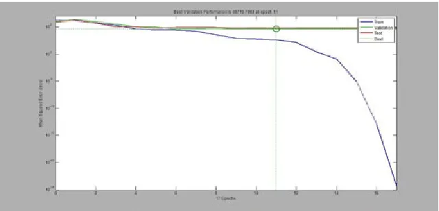
For purpose of approximation of 162 data, 70% of data have been considered as training data and 30% of them have been considered as experimental data. Based on presented modeling, mean squared errors for all data has been equal to 133. In Fig. 2, the diagram indicates error levels of training and examining in 17 iterations.

Fig. 2.

0 20 40 60 80 100 120 140 160 180 500

1000 1500 2000 2500 3000

Number Of Models

del

ay

delay and NN Prediction

Exact NN

0 20 40 60 80 100 120 140 160 180

-100 -50 0 50

Number Of Models Prediction Errors

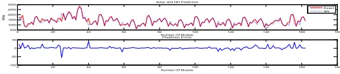
Fig. 3.

Comparing Actual Values and Predicted Value by Neural Network

0 20 40 60 80 100 120 140 160 180

500 1000 1500 2000 2500 3000

Number Of Models

del

ay

delay and NN Prediction

Exact NN

0 20 40 60 80 100 120 140 160 180

-100 -50 0 50

Number Of Models Prediction Errors

Fig. 4.

Error Percent Diagram by Neural Network

In Fig. 3, predicted delay values by neural network have been compared to output values of the software. Blue curve illustrates predicted delay rate by neural network and red curve indicates calculated values by the software. The diagram in Fig. 4 has also illustrated error percent of the network.

4.4. Approximating Delay Rate Using

Genetic Programming

All obtained data from the previous step have been analyzed using GP through Multigene Symbolic Regression and delay rate has been estimated. In GP, because of nature of the system and using evolution theory, there would be no need for determining effective data. Based on the data, 26 inputs have been

defined for the program and one output has been obtained from the program that is same delay rate. Accordingly, value of inputs in GP network is introduced equal to 26 inputs, which is according to inputs of the program based on Table 4 and Table 5.

GP algorithm would be stated as the primary population through random production. The formulas include functions, variables and fixed coefficients. Applied functions in the equations can be in different forms such as simple calculative operators; mathematical standard functions; conditional functions or logical functions. Due to the type of problem, equations can include numerical, conditional, logical, actual, vector and symbolic values or they can be multi-valued.

Table 4

Inputs of Genetic Programming in Dadman-Farahzadi

Dadman-Farahzadi _E-W

Ratio Cycle Length SBT

& L SBT SBL NBT & L NBT NBL WBT & L WBT WBL EBT & L EBT EBL

Table 5

Inputs of Genetic Programming in Darya-Farahzadi

Darya-Farahzadi _E-W

Ratio Cycle Length SBT

& L SBT SBL NBT & L NBT NBL WBT & L WBT WBL EBT & L EBT EBL

X26 X25 X24 X23 X22 X21 X20 X19 X18 X17 X16 X15 X2 X1

In order to estimate average delay, due to the type of data, different networks were created, so that effective parameters in the network can be determined in improving approximation. Number of gene, depth of each tree and also rate of primary population and number of generation have been the most important effective factors in approximation of the network. On the other hand, over magnification of the produced equation can cause it to have inadequate use. Hence, after repetitive modeling modes in form of try and error, primary

population has been considered equal to 100 people and number of generation period has been considered equal to 1000 periods. Applied functions include sinus, cosinus, and tangent, hyperbolic and symbolic function. Number of genes is equal to 10 and depth of trees has been considered to 10. For purpose of approximating 162 data, 70% of data have been considered as training data and 30% of them have been considered as experimental data. Data and output of the program have been presented in Table 6.

Table 6

Summary of Values and Outputs of Genetic Programming

10 Max genes 100 Population size

116.64 Training RMSE 1000 Number of generations

190.82 Testing RMSE 10 Max tree depth

1156.20 Time computing (sec) Inf Max nodes per tree

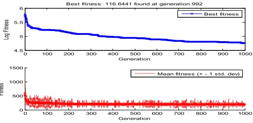
In Fig. 5, values of RMSE for predicted values have been traced based on GP. The upper diagram has illustrated RMSE in logarithm mode. In Fig. 6, RMSE values

have been illustrated in the diagram in simple form. As it is obvious, after generation 300, reduction of error level has too mild slope.

0 100 200 300 400 500 600 700 800 900 1000

4.5 5 5.5 6

Log F

itnes

s

Generation

Best fitness: 116.6441 found at generation 992

Best fitness

0 100 200 300 400 500 600 700 800 900 1000

0 500 1000 1500

Generation

Fit

nes

s

Mean fitness (+ - 1 std. dev)

0 100 200 300 400 500 600 700 800 900 1000 4.5 5 5.5 6 Log F itnes s Generation

Best fitness: 116.6441 found at generation 992

Best fitness

0 100 200 300 400 500 600 700 800 900 1000

0 500 1000 1500 Generation Fitnes

s Mean fitness (+ - 1 std. dev)

Fig. 6.

Diagram of Error Level while Training for 1000 Generation Periods (in Simple Form)

0 20 40 60 80 100 120 140 160 180

500 1000 1500 2000 2500 3000

Number Of Models

del

ay

Delay and GP Prediction

Exact GP

0 20 40 60 80 100 120 140 160 180

-100 -50 0 50

Number Of Models Prediction Errors

Fig. 7.

Diagram of Comparing Actual Values with Approximate Values for All Data

0 20 40 60 80 100 120 140 160 180

500 1000 1500 2000 2500 3000

Number Of Models

del

ay

Delay and GP Prediction

Exact GP

0 20 40 60 80 100 120 140 160 180

-100 -50 0 50

Number Of Models Prediction Errors

Fig. 8.

Diagram of Error Percent for All Data

In Fig. 7, predicted values by GP have been compared to outputs of the software. In the Fig. 8, error percent of predicted values by GP have been also traced. In Fig. 9 and Fig. 10, predicted values by GP in training

and experimenting modes have been traced separately and also RMSE value has been also depicted in the top of each diagram. Clearly, RMSE values in training are significantly lower than experiment.

0 20 40 60 80 100 120

0 2000 4000

y

Data point

RMS training set error: 116.6441 Variation explained: 91.5693 % Predicted y (training values)

Actual y (training values)

0 5 10 15 20 25 30 35 40 45

0 2000 4000

y

Data point

RMS test set error: 190.8238 Variation explained: 68.988 %

Predicted y (test values) Actual y (test values)

1 2 3 4 5 6 7 8

1000 1500 2000

y

Data point

RMS validation set error: 221.2002 Variation explained: -24.9325 %

Predicted y (validation values) Actual y (validation values)

Fig. 9.

0 20 40 60 80 100 120 0

2000 4000

y

Data point

RMS training s et error: 116.6441 Variation ex plained: 91.5693 % Predic ted y (training values ) Ac tual y (training values )

0 5 10 15 20 25 30 35 40 45

0 2000 4000

y

Data point

RMS tes t s et error: 190.8238 Variation ex plained: 68.988 %

Predic ted y (tes t values ) Ac tual y (tes t values )

1 2 3 4 5 6 7 8

1000 1500 2000

y

Data point

RMS validation s et error: 221.2002 Variation ex plained: -24.9325 %

Predic ted y (validation values ) Ac tual y (validation values )

Fig. 10.

Diagram of Comparing Actual Values with Approximate Values for Experimental Data

In Fig. 11, coefficient rate of each gene (tree) has been depicted in final equation of GP. Through comparing weights of each gene, in

fact percent of participation of each gene in final equation can be observed. Genes 1, 2 and 7 have the most share in the final equation.

Bias Gene 1 Gene 2 Gene 3 Gene 4 Gene 5 Gene 6 Gene 7 Gene 8 Gene 9 Gene 10

-2000 -1500 -1000 -500 0 500

1000 Gene weights

Bias Gene 1 Gene 2 Gene 3 Gene 4 Gene 5 Gene 6 Gene 7 Gene 8 Gene 9 Gene 10

0 0.5 1 1.5 2 2.5

3x 10-7 P value (low = significant)

R squared = 0.91569 Adj. R squared = 0.90743

Fig. 11.

Diagram of Illustrating Weight of Each Gene in the Presented Equation in GP

4.5. Presenting Generated Equation by GP

In this section, generated equation by the GP has been presented for each gene separately. As it is obvious, GP has generated 10 genes, which the maximum depth in each gene has

been considered to 10. Gene 1 to Gene 10 indicate 10 generated genes by the GP.

Eq. (3) indicates final equation of GP, which is in fact set of all expressed genes and total set of all Genes (Genes 1-10).

Gene 1=554,1 plog(x^8 )-1709,

Gene 2= -(569(x^10-1,0x^9+plog(cos(psqroot(x^1 )) )+(plog(psqroot(x^10-x^2-psqroot(x^17 ))))))/20

Gene 3=45,18 x^11-45,18 psqroot(plog(cos(x^1+x^16-plog(x^5 ) ) ) ) -45,18 psqroot(plog(cos(x^1+x^19-plog(x^8 ) ) ) )-45,18plog(cos(x^10-psqroot(x^17 ) ) ) Gene 4=16.22 x^13-16,22 psqroot(psqroot(x^10-x^19-plog(psqroot(x^10-x^2 ) ) ) )-16,22cos(x^1+x^4-cos(x^1+x^19-x^8 ) )-16,22 plog(cos(psqroot(x^1 )-x^17 ))

Gene 5=10,43 plog (cos(x^1+x^4-cosx^1+x^19-plog (x^8 ))))-10.43x^19 Gene 6=88,36x^2-88,36 psqroot (x^2-x^8)

Gene 7=1399(psqroot(psqroot(x^5 ))-1,0 plog(x^8 )) Gene 8=54(x^10-1,0 psqroot (x^17 ))

"Y=25,55x^10-21,63x^1+45,18x^11+16,22x^13+21,63x^14-10,43x^19+88,36 x^2+28,45x^9-88,36 psqroot(x^2-x^8 )-21,63plog(0,003127x^12-cos(x^24 ) )+1399,0psqroot(psqroot(x^5 ) )+10,43 plog(cos(x^1+x^4-cos(x^1+x^19-plog(x^8 ) ) ) )-16,22psqroot(psqroot(x^10-x^19-plog(psqroot(x^10-x^2 ) ) ) )-16,22 cos(x^1+x^4-cos(x^1+x^19-x^8 ) )+192,5cos(plog(x^5 )-cos(psqroot(x^5 )-psqroot(psqroot(x^19-x^11 ) ) ) )-28,45plog(cos(psqroot(x^1 ) ) )-28,45plog(psqroot(x^10-x^2-psqroot(x^17 ) ) )-45,18 psqroot(plog(cos(x^1+x^19-plog(x^5 ) ) ) )-45,18psqroot(plog(cos(x^1+x^19-plog(x^8 ) ) ) )-844,9 )-45,18psqroot(plog(cos(x^1+x^19-plog(x^8 )-54,0psqroot(x^17 )-16,22 plog(cos(psqroot(x^1 )-x^17

) )-45,18plog(cos(x^10-psqroot(x^17 ) ) )-1709,0 (3)

psqroot(a)=√(|a| )

plog(loga )=log|a|

4.6. Comparing Neural Network and GP

Here, results of neural network and GP have been compared to each other in summary.

Fig. 12.

Comparing Results of NN and GP

As it is obvious in diagram of Fig. 12, predicted values by the neural network and GP have desirable approximate.

Fig. 13.

In diagram of Fig. 13, values of error level of neural network and GP have been compared to each other. As it is obvious in the diagram, in some points both programs have high error level; although in some

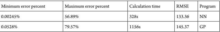
points one of the programs has lower error level than the other one. In general, neural network has lower error level than GP and this issue has been presented in Table 7 in summary.

Table 7

Comparing Neural Network and Genetic Programming

Minimum error percent Maximum error percent Calculation time RMSE Program

0.00245% 56.89% 328s 133.36 NN

0.0528% 79.57% 1156s 145.37 GP

As it is depicted in Table 7, generally in terms of both time of calculations and error level, neural network is in better situation than GP. However, presenting the formula by the GP is a brilliant feature of the network that can have better use than neural network.

4.7. Determining Values of Optimized

Inputs

Optimization has been conducted on both systems of NN and GP. In order to conduct optimization, “ga” base order in MATLAB software has been applied. Primary population rate and generation rate has been equal to 1000. Due to the presented optimized model by engineering software of Synchro, number of variables would be equal to 10 and all remained

variables would be 0. As the answer of the problem can’t be negative, this issue can be considered as limit of optimization problem. In addition, due to this issue that parameters are in form of integers, this issue should be also considered in the program. For this purpose, before entrance of variables to the target function that is same approximate network, they should be entered to the target function in form of integer and round up. Through this, obtained values by genetic algorithm would cause minimization of target function through becoming round up. Values of the current and optimized status of engineering software have been given to the two approximate networks (GP and NN) and obtained results have been compared to outputs of the software in Table 8.

Table 8

Comparing Calculated Delay Obtained from Software (SYNCHRO) and Two Approximating Networks (GP and NN)

Error percent

of GP Error percent of NN Delay calculated by GP & GA Delay calculated by NN & GA Delay calculated by SYNCHRO

9.97% 8.64% 1361.44 1131.07 1238 Current Situation

4.8. Validation of Proposed Algorithms

and Investigation of their Impacts on

other Parameters

For purpose of comparing proposed methods in terms of traffic index, the mentioned methods have been simulated in AIMSUN software. It should be mentioned that the software has been also applied for purpose of analyzing the current situation. In continue,

methods would be compared and evaluated based on different outputs of the software.

Finally, changing levels in traffic of the desired network in each method would be presented based on the current situation.

In Table 9, changing levels of traffic parameters have been estimated based on the current situation.

Table 9

Changing Level of Traffic Parameters Based on the Current Situation

Flow Density Speed Delay Stop Time Travel time

Current Situation 6450 49 7 554 461 299519

NN & GA 6672 45 8 458 363 242633

GP & GA 6679 52 11 553 459 236296

SYNCHRO 6996 51 12 487 487 328558

In Fig. 14, ranking of the proposed methods has been estimated in terms of imposed delay on the vehicles. Naturally, the method with less delay would be more desirable

than others. Therefore, the most desirable method in terms of delay can be combination of NN and GP that have the minimum delay rate.

Fig. 14.

Ranking Different Timing Methods in Terms of Imposed Delay on Vehicles

Ratio of flow to density indicates smooth flow of traffic in the network. The more the movement flow in the network is, the

versa, the less the density of the network is, the better performance of the network would be. Hence, the bigger the ratio is, the higher desirability of the network would be. In Fig. 15, ranking of proposed

methods has been presented based on flow to density ratio. According to the figure, in the combination of NN and GP, the network has the highest moving flow to density ratio.

Fig. 15.

Ranking Different Timing Methods in Terms of Flow to Density Ratio in Vehicles

Theoretically, every network that has lower travel time is more desirable in terms of traffic and vice versa, the more the speed of cars is in the network, the network would be more desirable in terms of traffic. On the other hand, in this software, travel time of those vehicles would be calculated that have been excluded from the network. Therefore, in those networks that have been blocked

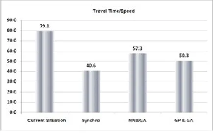
and vehicles have not been able to pass the network, less travel time has been obtained and this can’t be sign of desirability of the network. Hence, travel time to speed of cars ratio has been applied for purpose of evaluating models. Hence, the less the ratio is, the higher desirability of the network would be. In Fig. 16, ranking of proposed methods has been presented based on travel time to speed ratio.

Fig. 16.

5. Conclusion

Evaluation of outputs of combined algorithm of NN and GP and comparing it with outputs of SYNCHRO software has been conducted using AIMSUN software. Other results obtained from the study due to the conducted analyses on statistics and obtained results from model implementation are as follows:

1. Presented methods have been to some extent successful in regard with achieving their target that is determining optimized timing. Therefore, it could be mentioned that the methods can depict relative improvement compared to existed methods of SYNCHRO software and HCM regulation.

2. Artificial neural networks and genetic programming have had desirable performance in regard with predicting average delay imposed on vehicles under different timing combinations. The method has presented desirable answers for two studied intersections.

3. In general, both in terms of calculation time and error percent, neural network has better situation than genetic programming. However, presenting equation by genetic programming can be a brilliant feature of the network that can have better use than neural network.

References

Abdullahi, B.; Porwal, H.; Recker, W. 1999. Short Term Freeway Traffic Flow prediction Using Genetically-Optimized Time-Delay-Based Neural Networks, Institute Transportation Studies. California PATH Working Paper,

UCB-ITS, PWP-99-1.

Adacher, L. 2012. A global optimization approach to solve the traffic signal synchronization problem,

Procedia-Social and Behavioral Sciences. DOI: http://dx.doi. org/10.1016/j.sbspro.2012.09.841, 54: 1270-1277.

Alodat, M.; Al-Odat, I. 2013. Using Polygamy Technology with FL, GA and NN on Traffic Lights,

The International Journal of Engineering and Science (IJES), 2(7): 39-45.

Chang, J.; Bertoli, B.; Xin, W. 2010. New Signal Control Optimization Policy for Oversaturated Arterial Systems. In Proceedings of the Transportation Research Board 89th Annual Meeting, Washington D.C., USA. 20 p.

Dell’Orco, M.; Baskan, O.; Marinelli, M. 2013. A harmony search algorithm approach for optimizing traffic signal timings, Promet-Traffic & Transportation. DOI: http://dx.doi.org/10.7307/ptt.v25i4.979, 25(4): 349-358.

Girianna, M.; Benekohal, R. 2002. Dynamic Signal Coordination for Networks with Oversaturated Intersections, Transportation Research Record. DOI: http:// dx.doi.org/10.3141/1811-15, 1811: 122-130.

Hajbabaie, A.; Medina, J.C.; Benekohal, R.F. 2011. Traffic Signal Coordination and Queue Management in Oversaturated Intersection, NEXTRANS Project No. 047IY02. 108 p.

Hu, X.; Lu, J.; Wang, W.; Zhirui, Y. 2015. Traffic Signal Synchronization in the Saturated High-Density Grid Road Network, Computational Intelligence and Neuroscience, Article ID 532960. 1-11.

König, R. 2014. Enhancing Genetic programming for predictive modeling, Örebro: Örebro universitet. 240 p.

Searson, D. 2009. GPTIPS: Genetic Programming & Symbolic Regression for MATLAB. Available from Internet: <http://gptips.sourceforge.net>.

Searson, D.P.; Leahy, D.E.; Willis, M.J. 2010. GPTIPS: An Open Source Genetic Programming Toolbox for Multigene Symbolic Regression, In Proceedings of International MultiConference of Engineers and Computer Scientists (IMECS). 77-80.

Teodorović, D.; Šelmić, M.; Vukićević, I. 2014. Locating Hubs in Transport Networks: An Artificial Intelligence Approach, International Journal for Traffic and Transport Engineering. DOI: http://dx.doi.org/10.7708/ ijtte.2014.4(3).04, 4(3): 286-296.

Transportation Research Board. 2000. Highway Capacity Manual, Published by the National Research Council, Washington D.C.