finalre
port
p
Project code: NBP.231
Prepared by:
Teresa Eyre1, Annie Kelly1, Daniel Ferguson1, Col Paton2, Michael Mathieson1,
Giselle Whish2, Melanie Venz1, Jane Hamilton2, Jian Wang1, Rosalie Buck1 and Luke Hogan1 1. Department of Environment
and Resource Management 2. Department ofEmployment, Economic Development and Innovation
Date published: October 2011
ISBN: 9781741916393
PUBLISHED BY
Meat & Livestock Australia Limited Locked Bag 991
NORTH SYDNEY NSW 2059
Biodiversity Condition Assessment
for Grazing Lands
Meat & Livestock Australia acknowledges the matching funds provided by the Australian Government to support the research and development detailed in this publication.
Abstract
The primary purpose of the project was to develop and test a prototype procedure for the assessment of biodiversity condition of grazing lands. This would then complement the grazing land condition assessment framework used by the Grazing Land Management education package, which promotes sustainable management of grazed lands in northern Australia. To do this, comprehensive sampling of fauna, flora, habitat features and grazing land condition indicators was conducted at 171 sites. The sample sites were stratified across three different land types of southern Queensland (soft mulga, poplar box on alluvial and brigalow belah scrub), and broad condition states. The project culminated in a stand-alone product with three linked components including (1) a technical manual on the assessment of biodiversity condition ‘BioCondition’ (This publication has already been widely accepted is currently used by
professionals in the public and private sector); (2) a Biodiversity in Grazed Lands Toolkit, which
is comprised of seven ‘sub-kits’ including a simplified version of the technical BioCondition
Executive Summary
There is a strong demand for robust and practical approaches to assess resource condition, particularly in extensive grazing landscapes. A simple, rapid assessment approach is highly desirable as compared with a time-consuming and complicated, if thorough, approach, as it facilitates uptake of use by managers. The grazing land condition ‘ABCD’ framework of the EDGEnetwork Grazing Land Management education package is an example of an
assessment approach that has had widespread uptake by grazing land managers and is now a well established procedure in northern Australia. It uses a simple ‘ABCD’ rating, which is consistent with grazing land ecology concepts and sustainable livestock production. However, the framework currently does not address the assessment of condition relevant for biodiversity values.
The primary purpose of the Biodiversity Condition for Grazing Lands project was to develop and test a prototype procedure for the assessment of biodiversity condition that was complimentary to the ABCD grazing land condition assessment framework. To achieve this, a set of surrogate indicators of condition for biodiversity were selected and tested for three extensive, but ecologically different, land types in the Southern Brigalow Bioregion and Mulga Lands bioregion of southern Queensland. Testing involved the comprehensive sampling of fauna, flora, habitat features and grazing land condition indicators at 171 sample sites. The sample sites were stratified across three different land types of southern Queensland (soft mulga, poplar box on alluvial and brigalow belah scrub), and broad condition states.
For the majority of sites – across land types, landscape types and broad condition (i.e. remnant versus non remnant), there was close alignment between land condition and biodiversity condition classification. The assessment frameworks differed in their assessment of ‘good’ or functional condition (A or B grazing land condition; 1 or 2 BioCondition) predominantly in pasture and regrowth sites. That is, a site assessed as ‘A’ or ‘B’ grazing land condition was likely to be assessed in ‘3’ or ‘4’ BioCondition if the site had previously been cleared. At sites where remnant vegetation had been retained, ‘A’ or ‘B’ condition was mostly aligned with ‘1’ or ‘2’ condition. The response of biodiversity to classes representing grazing land condition (ABCD) and the prototype biodiversity condition approach (BioCondition; 1234) was determined using measures of species composition and species richness within broad taxonomic groups. As expected, the BioCondition framework did reflect variation in biodiversity values, albeit there was little discernible difference between classes 1 and 2. However, the ABCD framework did not reflect variation in species composition within tested fauna taxonomic groups (birds and reptiles), but did have some capacity to account for variation in perennial grass species composition.
Key attributes of the ABCD and BioCondition frameworks were tested against species richness and abundance of individual species indentified as increasers or decreasers. Those attributes which were both uncorrelated with other attributes and contributed to explaining much of the variation in species richness or individual abundance were selected as the key features for a rapid biodiversity condition assessment procedure, relevant to the brigalow and mulga lands bioregions. Acknowledgement by managers on the importance of these key features to biodiversity will greatly assist the conservation of species in grazing landscapes. We were able to show that the biodiversity in paddocks of open pasture, which are in A or B grazing land condition, can be greatly enhanced through the retention and maintenance of scattered keystone habitat features such as clumps of shrubs/regrowth, large trees and fallen woody material.
grazing land condition for biodiversity, reveal where condition for biodiversity and land management are similar and where they differ, and provide some insights on how to maintain or improve condition for biodiversity in the paddock and across the property. Components of the Toolkit can be used to demonstrate sustainable management for biodiversity to benefit grazing land managers in the marketplace and when competing for relevant funding. The toolkit was produced to support facilitators, extension officers and Natural Resource Management groups who work with grazing land managers involved in the management of grazing land production and biodiversity conservation. The toolkit can also be used directly by grazing land managers interested in biodiversity conservation, particularly those familiar with the concepts used in the EDGEnetwork Grazing Land
Management and Stocktake education and training packages.
Contents
Page
1
Background
... 8
1.1
Introduction
...8
1.2
Grazing land condition (ABCD framework)
...9
1.3
Biodiversity condition (1234 BioCondition framework)
...11
2
Project Objectives
... 13
3
Methodology
... 15
3.1
Study region
...15
3.1.1
The Mulga Lands
...15
3.1.2
Brigalow Belt South
...15
3.2
Site Selection
...16
3.3
Fauna surveys
...20
3.3.1
Birds
...20
3.3.2
Reptiles
...21
3.3.3
Incidental vertebrate records
...21
3.4
Flora surveys
...22
3.5
Site-based habitat features
...22
3.5.1
Trees and shrubs
...23
3.5.2
..
23
Native perennial grass basal area - preferred and intermediate species
3.5.3
Litter cover
...24
3.5.4
Cryptogram cover
...24
3.5.5
Fallen woody material
...25
3.5.6
Landscape Function Indicators (LFI) of soil and pasture condition
...25
3.5.7
Landscape Function Zones (LFZ)
...25
3.6
Landscape-scale features
...26
3.6.1
Patch size
...26
3.6.2
Connectivity
...27
3.6.3
Context
...27
3.6.4
Distance to permanent waterpoint
...28
3.8
Biodiversity condition assessment
...30
3.9
Landholder or land manager surveys
...30
3.10
Analyses
...30
3.10.1
The relative importance of key habitat features
...31
3.10.2
Species richness and ABCD and 1234 condition classes
...32
3.10.3
Species composition and ABCD and 1234 condition classes
...32
3.11
Trial to map condition using remotely sensed imagery
...32
4
Results and Discussion
... 33
4.1
General fauna results
...33
4.1.1
Amphibians (Frogs)
...34
4.1.2
Reptiles
...34
4.1.3
Birds
...36
4.1.4
Mammals
...38
4.2
General flora
...39
4.3
Biodiversity condition (1234) and Grazing land condition (ABCD)
44
4.3.1
Where the assessment of land and biodiversity condition differed
...45
4.3.2
Where ABCD and 1234 condition classes aligned
...46
4.3.3
Where ABCD and 1234 differed by two to three condition classes
...47
4.4
The relative importance of key habitat features
...49
4.4.1
Landscape-scale key features
...49
4.4.2
Site-based key features
...49
4.5
Key features, increasers, decreasers and species richness
...53
4.5.1
Miners and small passerine birds
...53
4.5.2
Shrub cover
...54
4.5.3
Large live trees
...55
4.5.4
Distance to waterpoints
...56
4.6
Biodiversity and ABCD and 1234 condition classes
...56
4.6.1
Grasses and condition classes
...56
4.6.2
Forbs and condition classes
...62
4.6.3
Reptiles and condition classes
...63
4.6.4
Diurnal birds and condition classes
...69
4.7
Testing the value of the rapid 1234 assessment
...76
4.7.2
Tree canopy cover
...77
4.7.3
Shrub canopy cover
...77
4.7.4
Large live trees
...77
4.7.5
Fallen logs
...78
4.7.6
Preferred and intermediate grass cover
...78
4.7.7
Litter and weed cover
...78
4.7.8
Landscape attributes
...79
4.7.9
Overall rapid scores and condition classes
...79
4.8
Mapping condition in the mulga lands
...81
4.9
Quantification of ABCD rapid assessment
...82
4.9.1
Mulga region – soft mulga sites
...83
4.9.2
Brigalow belt south region – brigalow-belah sites
...83
4.9.3
Brigalow belt south region – poplar box on alluvial plains sites
...87
5
Success in Achieving Objectives
... 88
5.1
Success in Achieving Objectives
...88
6
... 90
Impact on Meat and Livestock Industry – now and
in five years time
7
Conclusions and Recommendations
... 91
8
Bibliography
... 93
Appendix 1 Regional ecosystems sampled ... 100
Appendix 2: Benchmark documents ... 102
Benchmarks 11.3.2
...103
Benchmarks 11.9.5
...105
Benchmarks soft mulga
...106
Appendix 3: Fauna species by land type ... 108
Appendix 4: Plant species by life form by land type ... 118
Appendix 5: Biodiversity Condition Toolkit for Grazed
Lands ... 133
1 Background
1.1 Introduction
The management of native vegetation to produce services such as food and fibre has meant that an estimated 62% of Australia’s native vegetation has been modified by agricultural and grazing enterprises (Thackway and Lesslie 2006). Knowledge of the extent of native vegetation by broad structural and floristic type is therefore considered integral for natural resource planning, management and environmental reporting. Consequently, vegetation-mapping programs to describe structural and floristic type have been conducted across the majority of the states and territories of Australia. This has been broadly captured and described at a national scale by the National Vegetation Information System (NVIS) framework (ESCAVI 2003). However, vegetation description and mapping at the regional scales is much less consistent between Australian state and territory boundaries, as well as within. An exception is Queensland, which is unique in that it is the only Australian jurisdiction to have a statewide ecosystem mapping program1 at a regional scale (1:100 000). This is regularly updated to monitor change in extent (Accad et al. 2006) using the
Statewide Land and Tree Study2 (Kuhnell et al. 1998) as a primary input. In Queensland, the regional ecosystem mapping is now being used to underpin the mapping of land types – an important information component of grazing land management.
Compared with vegetation extent, the assessment of vegetation condition is considerably
less well documented in Queensland, and indeed most of Australia. It has only been relatively recently that policy demands and expectations have conceptualized vegetation condition as a major component of native vegetation management, primarily to assist decision-making for developmental approvals, incentive payments and market-based investments (Keith and Gorrod 2006). Regional Natural Resource Management groups are also interested in vegetation condition, given its recent identification as a national environmental indicator for reporting targets (MEWG 2004). At the property scale, land managers are increasingly becoming aware of the challenge to demonstrate duty of care (Bates 2001; Neldner 2006), and indeed the assessment of condition for the purpose of lease renewal is now undertaken in Queensland under the Delbessie Agreement (DERM 2010).
A procedure to effectively assess vegetation condition is paramount to the implementation of these decision-making and reporting schemes, including implementation of off-sets and biobanking schemes and comprehensive environmental accounts (Hawke 2009). The ability to assess and monitor vegetation condition is also essential for governments to administer legislation relating to the landscapes and biodiversity covered by their jurisdiction. In Queensland, this legislation includes the Nature Conservation Act 1992, Land Act 1994, Environmental Protection Act 1994, Coastal Protection and Management Act 1995 and Vegetation Management Act 1999. In addition, premium markets are likely to
develop in the future for properties demonstrating sustainable production (Neldner 2006).
The use of the term ‘condition’ as it is generally used by policy and management, is underpinned by the assumption that its assessment will represent a measure of ecological composition, structure and function (sensu Noss 1990) along a continuum of ‘poor’ to
‘good’, relative to some desired state or potential. However, what the condition measure
1
represents is context dependent. One of the earliest definitions of condition was developed relative to grazing land management of rangelands, as the “health or productivity of both soil and forage of a given range, in terms of what it could or should be under normal climate and best practicable management” (Society of American Foresters 1944). Since then, the development of conceptual frameworks to better reflect ecological complexity and thinking, as well as the expansion of applications to which the concept of condition is often attached (e.g., Westoby et al., 1989), has led to much current confusion and ambiguity regarding
what is meant by ‘condition’ (Keith and Gorrod, 2006).
It is therefore important to be clear regarding the definition of ‘condition’ and the objective of any assessment as the approach used, the attributes to measure, and the outcome of the assessment will vary between contexts as a matter of necessity (Oliver et al. 2002). That is,
the measure will depend upon whether the objective for the condition assessment is for production, biodiversity or aesthetic purposes (Keith and Gorrod 2006; Gibbons and Freudenberger 2006). For instance, recent work in the savanna rangelands has shown that the concept of condition for productive grazing land only partially represents condition for biodiversity values (Fisher and Kutt 2007).
Ecology is complex, with many drivers and interactions and variable responses. Consequently, many indicators, surrogates and attributes have been suggested for use in rangeland assessment and monitoring (Smyth and James, 2004). However, a simple, rapid assessment approach is highly desirable as compared with a time-consuming and complicated, if thorough, approach, as it facilitates uptake of use by managers (Andreasen
et al. 2001). Accordingly, a number of recently developed condition assessment tools have
utilised a key set of attributes or surrogates of that can be rapidly measured in the field (Gibbons and Freudenberger 2006). From a grazing land management perspective, the ABCD framework is one, and from a biodiversity perspective, the BioCondition framework - developed for this project - is another.
1.2 Grazing land condition (ABCD framework)
Grazing Land Management (GLM) education packages define grazing land condition as “the capacity of land to respond to rain and produce useful forage” (Pickup et al. 1994;
Chilcott et al. 2003). The concept underpinning the definition is that ecological processes,
such as nutrient cycling, are maintained through variable rainfall periods to ensure stable responses by pasture species relative to livestock carrying capacity (Karfs et al. 2009a).
The associated ABCD grazing land condition framework (Chilcott et al. 2003), developed
from existing knowledge and long term grazing trial data (e.g. Ash et al. 2002), allows the
differentiation between four grazing land condition classes, relative to a particular land type (Table 1). Indicators used in the ABCD framework include:
soil condition: the capacity of the soil to absorb and store rainfall, store and cycle nutrients, provide habitat for seed germination and plant growth, and to resist erosion. It is measured by the condition of the soil surface, which is influenced by the amount of ground cover over time, and the signs and extent of erosion.
ground cover per se is not an indicator of land condition as its presence or absence can fluctuate with season and events such as fire.
It is the combination of these two factors (soil and pasture condition) that determines a land condition rating. Woodland condition (see below) is measured by measuring tree basal area (TBA).
woodland condition: the capacity of the woodland to grow pasture, cycle nutrients and regulate groundwater. It is measured by measuring the density and trunk size of trees and shrubs present using a variation of the Bitterlich technique.
Table 1: Features of ABCD grazing land condition classes. A condition has all the features listed, while other condition classes exhibit one or more of the listed features.
Grazing land condition class
Features
A
High density and good cover of perennial grasses dominated by 3P species (perennial, productive and palatable) for a particular land type
Little bare ground (usually <30%)
Few or no weeds
Good soil condition; no erosion and good surface condition
High organic matter
Little woody thickening
B
Some decline in the health and/or density of 3P grasses; an increase in other less favoured or weed species
Some decline in soil condition; some signs of previous erosion and/or increased bare ground (usually >30% but <60%)
C
Moderate to low density of preferred grasses or moderate density of intermediate grasses
High numbers of annual grasses and forbs,
Many weeds
Some erosion
Often poor ground cover (<60%)
Some woody thickening
D
General lack of any perennial grasses or palatable forbs
Severe erosion or scalding, resulting in restricted plant growth
High numbers of weeds and annuals
Thickets of woody plants or weeds cover most of the area
1.3 Biodiversity condition (1234 BioCondition framework)
The use of the reference condition approach underpins most procedures developed in Australia for vegetation condition assessment for biodiversity. The referential approach compares an indicator or attribute at the assessable site with a value, or range of values expected for that site if it was in a state of the desired condition – usually a pristine state free from threatening factors – known as the ‘reference condition’ (Karr and Chu 1999; Bailey et al. 2004). The use of reference conditions has also been widely used for
assessment of water quality (Negus and Marsh 2006), and is rapidly being embraced by terrestrial assessment systems as it provides an objective means of comparison within and between vegetation ecosystems.
The reference approach can potentially be criticized as being the construct of another Clementsian-based successional model, but this will depend on what state is used as the ‘desired’ state of condition for comparison (Gibbons and Freudenberger 2006). The BioMetric approach (Gibbons et al. 2008) aims to avoid this criticism by providing a range of
values as the benchmark for vegetation communities, representing the natural alternative states that the community may display as a consequence of environmental variation or natural disturbance. However, in general, the ‘historical’ pristine natural state, with absence of post-European human disturbance is usually used as the reference state (e.g. Parkes et al. 2003). The use of sites in a ‘pristine’ state is unrealistic, given that impacts from
post-European settlement management are widespread. Furthermore, it is extremely unlikely that a given patch of vegetation could be restored to historical states (Hobbs and Norton 1996; Oliver et al. 2002). Sites that have been least impacted by local threats should be of
increased value for aspects of biodiversity, thus should constitute the best available benchmarks, or ‘best-on-offer’ (Landsberg and Crowley 2004). This is the approach that has been adopted for this project, and used in BioCondition (Eyre et al. 2011).
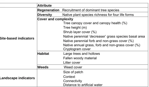
BioCondition is broadly constructed of three components:
1. A set of site-based and landscape-scaled attributes – which act as surrogates of
biodiversity values. These attributes were selected based on their known or perceived surrogacy for aspects of biodiversity and representation of ecological processes relative to composition, structure and function, their relevance and applicability for a range of ecosystem types and condition states, the relative ease with which they can be assessed and their educational appeal (Table 2).
2. Benchmarks – are quantitative values for each attribute obtained from a set of
Best-on-Offer (BOO) ‘reference’ sites for a particular regional ecosystem or land type. For this project, benchmark data were derived from six to seven BOO sites located in each of the three target land types (brigalow-belah woodlands on sedimentary; soft mulga woodlands; and poplar box woodlands on alluvial; see Appendix 1).
3. Rating system – based on the relative value of an attribute to the benchmark
Table 2: Assessable indicators used in BioCondition to derive 1234 condition ratings
Attribute
Regeneration Recruitment of dominant tree species
Diversity Native plant species richness for four life forms Cover and complexity
Tree canopy cover and canopy health (%) Tree height (m)
Shrub layer cover (%)
Native perennial ‘decreaser’ grass species basal area Native perennial forb and non-grass cover (%)
Native annual grass, forb and non-grass cover (%) Cryptogram cover
Habitat Large trees and hollows
Fallen woody material Litter cover
Site-based indicators
Weeds Weed cover
Size of patch Context
Landscape indicators
Connectivity
2 Project Objectives
The primary purpose of the project was to develop and test a prototype procedure for the assessment of biodiversity condition of grazing lands, to complement the land assessment framework used by the Grazing Land Management education package, which promotes sustainable management of grazed lands in northern Australia. The specific objectives of the project were to:
1. Provide a prototype toolkit (and corresponding set of presentations in powerpoint format), for the rapid assessment of biodiversity condition on grazing lands that is compatible with the grazing land condition (ABCD) assessment framework used in the GLM education package, and which includes materials for;
a. The rapid assessment of biodiversity condition (BioCondition);
b. Understanding biodiversity condition and its relationship to grazing land condition;
c. The significance of the BioCondition ratings for property and regional biodiversity, and;
d. Management options for maintaining or improving biodiversity in the grazed lands of southern Queensland.
2. Specify a set of surrogate indicators of condition for biodiversity on grazing lands, and their benchmark values, for a range of regional ecosystems occurring on grazing properties in the Southern Brigalow and Mulga regions of southern Queensland.
3. Establish relationships between the surrogate indicators and selected elements of biodiversity (e.g. persistence of identified decreaser species or species groups, for a range of flora and fauna) in the study regions.
3 Methodology
3.1 Study region
This project was conducted within two Interim Biogeographic Regionalisation of Australia (IBRA) bioregions within Queensland, the Mulga Lands and Brigalow Belt South bioregions. Within the two bioregions, sites were restricted to the Soft Mulga land types which are broadly distributed to the east of the bioregion, and the Brigalow-belah on sedimentary and poplar box on alluvial land types distributed towards the west of the Brigalow Belt South bioregion (Figure 2).
3.1.1 The Mulga Lands
The Mulga Lands bioregion covers approximately 18.1 million hectares, and constitutes 12.5% of Queensland. The Mulga Lands bioregion is dominated by flat to undulating plains and low ranges supporting a range of mulga Acacia aneura woodlands. Poplar box Eucalyptus populnea and other eucalypt species codominate with mulga in the more
easterly parts of the bioregion, which receive higher rainfall (Wilson, 1999). The bioregion is subject to extremely variable rainfall patterns and relatively frequent droughts.
The primary land use in the Mulga Lands bioregion is grazing by sheep, cattle and increasingly, goats. Mulga provides a significant reserve of forage for sheep and cattle particularly during drought, although supplement feeding is required to maintain animal condition during prolonged feeding. The landscape in the Mulga Lands is predominantly intact, except towards the east where intensive land clearing has occurred prior to cessation of broadscale land clearing at the end of 2006. The majority of remnant vegetation clearing in Queensland between 2001 and 2003 occurred in the Mulga Lands bioregion (55% of clearing in Queensland; Accad et al. 2006). Land resource surveys conducted in the region
indicated that 20% of the area has substantial cover of unpalatable woody perennials in the understorey, and close to 30% of the areas has been affected by sheet erosion (Beale, 1994).
3.1.2 Brigalow Belt South
The Brigalow Belt South covers approximately 22.7 million hectares, comprising approximately 15% of Queensland. The bioregion has a subtropical climate although droughts are common. Rainfall tends to decrease from the eastern to western areas of the bioregion, but is summer dominant and highly variable. The bioregion is characterized by brigalow Acacia harpopylla which occurs in forest and woodland formations on clay soils.
Eucalypt forests and woodlands and cypress pine Callitris glaucophylla forests are also
dominant ecosystems in the bioregion (Young et al. 1999).
Broadscale clearing of brigalow communities occurred as part of grazing land development schemes initiated in the 1960’s (Young et al. 1999). By 1990, 86% of the original extent of
brigalow and belah Casuarina cristata scrub had been cleared. In the Dalby, Chinchilla and
Goondiwindi areas, brigalow/belah communities had decreased by 96% (Smyth 1997). The other ecosystem that has been extensively cleared in the bioregion has been poplar box
Eucalyptus populnea dominant communities. Approximately 70% of the pre-clear poplar box
woodlands have been cleared for stock grazing, and much of the remaining 30% is also grazed. are now grazed pasture land. The establishment of buffel grass Pennisetum ciliare
Figure 2: Broad study area showing delineation of the Mulga Lands and Brigalow Belt South bioregions. Hatched area shows the area within which sample sites were located. Inset shows the distribution of the three target landtypes across southern Queensland.
3.2 Site Selection
Across the two bioregions, three distinct land types were targeted to sample across high and low productivity for grazing; soft mulga in the Mulga Lands bioregion; and poplar box on alluvials and brigalow/belah scrub land types in the Brigalow Belt South bioregion. Eleven land types have been identified in the Mulga Lands bioregion (Whish (Ed.) 2010). In the region the most widely referred to land types include “soft” mulga, “hard” mulga and “sandplain” mulga. Soft mulga generally occurs to the east of the Warrego River, and hard mulga is distributed to the west. For the purposes of this project, soft mulga land types were targeted for survey. We aligned the soft mulga land type with relevant regional ecosystems, which have been described and mapped by the Queensland Herbarium (EPA 2005). Eleven regional ecosystems were identified as representing soft mulga land types. These were then mapped to demonstrate distribution in the bioregion for property selection.
for sampling; poplar box on alluvials land type and the brigalow/belah scrub landtype. These were selected due to their significant pre-clear and remnant extent and value as productive grazing land. A description of the regional ecosystems targeted to sample the soft mulga, brigalow belah scrub and poplar box land types is provided in Appendix 1.
The design used for site selection in the study area was based on a stratification of land type by landscape type by management type and by grazing land condition plus BOO condition for biodiversity (see Table 3 for definitions of the stratification variables used). A landscape was defined as a circular spatial extent encompassing 314 ha, centred on the sample site. Four landscape management types were selected for sampling in each land type; the conservation landscape, sampling 1) remnant vegetation in an intact landscape;
the mixed landscape sampling 2) a patch of remnant vegetation in a fragmented
landscape (e.g. Figure 3); and the production landscape, sampling both 3) pasture and 4) regrowth vegetation in a fragmented landscape. In the soft mulga fodder harvesting is
another form of pastoral management. Therefore, in this land type the production landscape sampled included 3) regrowth and/or pasture and 4) stump cut (lopped or
thinned for fodder).
We used the 1:100 000 remnant and pre-clear regional ecosystem mapping to delineate remnant and pre-clearing extent of the regional ecosystems selected to represent the three land types of interest. We also used a combination of the pre-clear regional ecosystem mapping and the Statewide Land and Tree Study (SLATS) woody cover mapping to delineate areas of potential regrowth or disturbed woody component for each of the three land types.
Figure 3: Example of the remnant vegetation in regrowth/cleared landscape. Dark green = mapped remnant vegetation, light green = pre-cleared vegetation, blue = potential regrowth / woody component from SLATS mapping.
In selecting and locating sites in the field, the following rules were followed;
a. Sites were located a minimum of 1 km apart, to avoid spatial autocorrelation issues associated with far-ranging taxa (birds);
b. Sites were located, as much as practicable, > 100 m from the edge of pasture / regrowth / remnant boundaries;
c. Sites were located wholly within paddocks i.e. sites did not cross fencelines; d. Sites were located > 200m from waterpoints.
Table 3: Definitions of stratification variables used
Stratification Definition Land type
Soft mulga Regional ecosystems: 6.5.1, 6.5.7, 6.5.9, 6.5.10, 6.5.11, 6.5.14, 6.5.18 (see Appendix 1 for description)
Brigalow/Belah Scrub Regional ecosystem 11.9.5 (see Appendix 1 for description) Poplar Box on alluvials Regional ecosystem 11.3.2 (see Appendix 1 for description) Landscape scale
Fragmented Remnant vegetation incorporates 10 to 30% of area within a 1-km radius landscape
Intact Remnant vegetation incorporates > 70% of the area within a 1-km radius landscape
Management (site scale)
Remnant vegetation Overstorey canopy cover is > 50% of the benchmark value for that regional ecosystem and median overstorey canopy height is > 70% of the benchmark value for that regional ecosystem.
Pasture Cleared for pasture growth. No (or minimal) regrowth or woody component (except in the mulga lands), and can be sowed to exotic species.
Regrowth Woody cover of appropriate ecosystem is present either in regeneration/regrowth phase, or has been disturbed through thinning (selective lop fodder feeding in mulga, thinning in brigalow and poplar box).
Condition
BOO Best-on-offer vegetation condition for biodiversity. Best available reference condition where attributes of the vegetation are within the range of natural variability and with relatively little evidence of modification by humans since European settlement.
AB AB Grazing Land Condition defined as good to fair ability of land to respond to rain and produce useful forage (Chilcott et al. 2003)
Table 4: Stratification table showing the treatments and number of sites selected for each
Land type Landscape Management Condition state Strata unit
No. sites
Brigalow-belah on sedimentary intact remnant Preferably ungrazed / light BOO 1 6
Conservation landscape AB 2 6
CD 3 6
fragmented landscape sampling remnant Remnant can be grazed AB 4 6
Mixed landscape CD 5 6
fragmented landscape sampling non-remnant Pasture (native or sown to buffel) AB 6 6
Production landscape CD 7 6
Brigalow regrowth or disturbed AB 8 6
(e.g. heavy thinning) CD 9 6
Soft Mulga intact remnant Preferably ungrazed/light BOO 10 7
Conservation landscape AB 11 7
CD 12 7
fragmented remnant AB 13 7
Mixed landscape CD 14 7
fragmented non-remnant Previously pushed AB 15 7
Production landscape (mulga regrowth) CD 16 7
Disturbed/thinned (lopped/ AB 17 7
axe cut / chainsaw) CD 18 7
Poplar box intact remnant Preferably ungrazed/light BOO 19 6
(alluvial) Conservation landscape AB 20 6
CD 21 6
fragmented remnant AB 22 6
Mixed landscape CD 23 6
fragmented non-remnant Pasture (native or sown to buffel) AB 24 6
Production landscape CD 25 6
Poplar box regrowth or disturbed AB 26 6
(e.g. heavy thinning) CD 27 6
3.3 Fauna surveys
Quantitative data on diurnal birds and reptiles was collected over two sampling periods, during spring and again during autumn. Repeated surveys for each taxonomic group were conducted at the same sites, to increase the probability of detection.
For this project diurnal birds and reptiles were targeted for survey because these taxa:
1. are known to be sensitive to variation in floristic and structural change in the mulgalands and brigalow belt bioregions
2. have broad distributions and are more likely to be detected relative to other taxonomic groups in the region (e.g. arboreal marsupials are naturally uncommon in the region; small ground-dwelling mammals tend to occur in pulses).
3. can be surveyed using relatively standardised and time efficient methods, which allows more sites to be surveyed.
All fauna survey techniques used in this study was endorsed by the Queensland Department of Environment and Resource Management Animal Ethics Committee (Approval number SRAEC0014).
All fauna sampling was based on a 1 ha (100 m x100 m) site (Figure 2). BioCondition and floristic sampling occurred on a randomly chosen 100 m x 50 m plot (A or B), located either side of the central N-S transect.
50 m
50 m
50
m
50
m
A2 herp search (50 x 50 m)
Habitat assessment (100 x 50 m)
N
Figure 4:Fauna sampling site layout
3.3.1 Birds
At each site, diurnal bird surveys were conducted within a 100 m x 100 m quadrat. The bird survey methodology was based on extensively used protocols developed for the Australian rangelands (Woinarski and Ash, 2002; Hannah et al., 2007; Kutt and Woinarski, 2007). Birds
Pit trap array 5
A1 herp search
were sampled over two six-day survey periods, one during ‘spring/summer’ (September to December) and again during ‘summer/autumn’ (February to May) during 2007 and 2008. During each survey period, birds were sampled in six, 10-min counts per quadrat, twice during the ‘early morning’ (<2 h after sunrise), twice during the ‘late morning’ (between 2- and 4-h after sunrise) and twice during ‘other’ times of the day (between 4-h after sunrise and 2-h before sunset). All surveys were conducted on different days by one of two observers on fine, calm days. Only birds seen or heard within the quadrat were counted. Birds flying over the quadrat were excluded, unless they were observed to be actively hawking or foraging within the quadrat.
Counts for each species were summed across the 12 quadrat samples to give a relative abundance for each site. Species richness was recorded as the number of species detected at least once at each site.
3.3.2 Reptiles
Two general techniques were used to survey for reptiles – pit trapping and active herpetofauna searches. Pit trapping involved using an array of four pit traps and six funnel traps on the sample plot in a T-shape pattern, as per the plot layout in Figure 2. Twenty-litre plastic buckets were used as pit traps, which were connected via drift-fence at 7.5 m intervals.
Active searches for herpetofauna were conducted over two survey periods (spring and autumn), on the 100 m x 50 m plot not selected for floristic measurements. The plot chosen for active herpetofauna searches was divided into two 50 m x 50 m quadrats – with A1 searched during the first period and A2 searched during the second survey period (Figure 4). This is done to eliminate the effect of the destructive active searches on the microhabitat used by the reptiles (e.g. logs, burrows, leaf litter etc).
Each quadrat is actively searched five times for herpetofauna (reptiles and frogs). Three active diurnal searches (approximately two in the morning and one in the late afternoon) along with two nocturnal searches (conducted at night using headtorches and, to a lesser extent, spotlights). Each search is conducted for 20 person-minutes (generally 2 persons x 10 minutes). The active diurnal searches involve scanning for active reptiles as well as turning rocks and logs, raking through leaf litter, looking under bark and in crevices looking for more cryptic reptile species. Nocturnal searches are, however, predominantly observational with little destructive searching. Nocturnal searches involve scanning for active reptiles, looking for eyeshine, and listening for signs of activity.
The number of individuals of each reptile species seen while searching is recorded along with any mammals or other fauna, scats, bones and other signs where these can confidently be attributed to species. A total abundance score for each species was derived from the sum of all counts from trapping and searches.
3.3.3 Incidental vertebrate records
3.4 Flora surveys
Ground floristics and attributes of ground cover were assessed within ten 1 x 1 m subplots located along the centre transect. The number and cover (%) of each flora species located within the subplot was recorded. The broad cover categories followed that described in BioCondition; native grass; native non-grass; native shrubs < 1 m height; non-native grass; non-native non-grass; fine litter < 10 cm diameter; rock; bare ground; cryptograms and other. Shrubs and small trees 2–20 cm DBH and > 1 m height are recorded in the 50 x 10 m subplot, and counted by species. Shrub canopy cover and Tree canopy cover is estimated along the 100m transect. All trees > 20 cm DBH are recorded in the 100 x 50 m area. The following characteristics are noted for each tree measured; species, diameter, whether it is dead or living, size and number of hollows.
Life forms discussed in this report included trees, shrubs (woody species usually 1.5-4 m in height and generally multi-stemmed, also including mistletoe), vines (woody), forbs (all herbaceous species including rushes, creepers, trailers and non-woody climbers), grasses (Poaceae), sedges (Cyperaceae) and ferns. The tallest and mid layers were composed of tree, vine and shrub species while the ground layer consisted of forb, grass, fern, sedge and shrub species. The assemblages of all species at each site were collated. Nomenclature used follows that of Bostock and Holland (2007). When identification to species or genus level was not possible, the specimen was identified to genus or family level.
3.5 Site-based habitat features
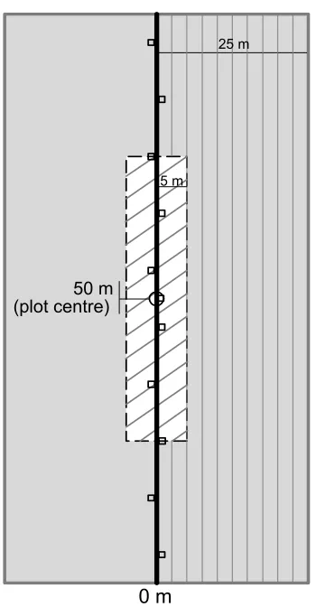
Field assessment of site based indicators selected for testing, as well as other attributes not selected but likely to provide habitat value for biodiversity (e.g. rock cover) or quantify disturbance levels (e.g. stumps) were conducted on one occasion at each site. The habitat assessment plot coincided with the fauna assessment plots. The habitat assessment site constituted a 100 m x 50 m fixed area plot, within which were nested a series of sub-plots required for specific habitat assessments (Figure 5). A total of five sub-plots were used to assess the habitat characteristics of each site, and are summarised as follows:
1. 100 x 50 m area: recorded all trees > 20 cm Diameter at Breast Height (DBH), all stumps > 5 cm diameter (plot size can vary depending on the density of stumps), and site information and disturbance;
2. 100 x 25 m area: recorded all coarse woody debris > 10 cm diameter (plot size can vary depending on the density of logs);
3. 100 m transect: recorded tree canopy cover, shrub canopy cover. 4. 50 x 10 m area: recorded all trees and shrubs 2 – 20 cm DBH.
100 x 50 m
- >30 cm DBH tree measurements - Tree layer floristics
- Site information and disturbance - Stumps information
50 x 10 m
- Shrub layer floristics - Ground layer
- 5-30 cm tree measurements 50 m
(plot centre)
100 x 25 m
- Fallen woody material
0 m
25 m
5 m
10 x 1 x 1 m plots - Organic litter - Ground cover
- Ground layer floristics
No
100 m Transect line - Tree canopy cover
Figure 5: Habitat assessment area and layout
3.5.1 Trees and shrubs
All trees > 20 cm DBH were recorded in the 100 x 50 m area. The following characteristics were recorded for each tree measures; species, diameter, whether it is dead or living, size and number of hollows. Tree canopy cover was assessed as the percent canopy cover of each tree whose projected canopy intersects the 100 m transect. The approach uses the line intercept method and treats each canopy as solid, i.e. continuous leaves with no light gaps) (Greig-Smith 1964). The vertical projection of the tree canopy and the height of each tree intercepted along the 100 m transect was recorded. The total length of the projected canopy was then divided by the total length of the tape to give an estimate of percent canopy cover for the tree layer. The health of the canopy of each tree intercepting the transect was assessed on a 1 to 4 scale (Eyre et al. 2011). The average height of the tree canopy was
also estimated. Shrubs and small trees 2 to 20 cm DBH and > 1 m height were recorded in the 50 x 10 m subplot, and counted by species. Shrub canopy cover was estimated as described for tree canopy cover.
3.5.2 Native perennial grass basal area - preferred and intermediate species
experimental measure used to assess grazing land pasture condition (DPI&F 2006). The preferred approach focuses on the assessment of "decreaser species" or preferred and intermediate species (which decline under heavy grazing), as opposed to “increaser species” and non-preferred species (which increase under heavy grazing). Each grass species encountered was identified as a preferred or intermediate species based on the respective land type documents.
Figure 6: Crown cover of grass tussock (from DPI&F 2006).
Two methods were used to assess grass basal area, a detailed method and a rapid method. The detailed method involved the assessment of the number, basal area size, via measurement of diameter of the tussock base and species of all grass tussocks within each of 10 quadrats (whose size was determined by the spatial arrangement of tussocks e.g. how spread out they are – quadrat sizes were either 1m2, 2m2 or 4m2). From this sample the Basal area of perennial decreaser grass species was determined. The second, more rapid method involved assessors literally “walking the transect line”. At each metre point along the 100m transect line, assessors recorded whether the point on the tape had struck the base of a grass species tussock. Grasses were identified to species.
3.5.3 Litter cover
Litter is a key habitat component for wildlife and woodland functioning. Leaf and woody litter protects the soil from erosion and its decomposition provides continual nutrient supply into the ecosystem. It supports a diverse range of invertebrates which in turn provide a food source for vertebrate species. Litter cover is considered one of an important minimum set of indicators to be included in a patch-scale, species-level biodiversity assessment (Oliver et al.
2007).
For the field assessment, litter was defined as including both fine and coarse organic material such as fallen leaves, twigs and branches < 10 cm diameter. Litter cover was assessed in each of the 10, 1x1m quadrats. An overall value of litter cover for each site was the average value of the 10 quadrat assessments.
3.5.4 Cryptogram cover
A cryptogram is a broad term for a plant which reproduces by spores, and includes groups such as algae, lichens, mosses, ferns and liverworts. They occur on stable surfaces and are considered to assist with the stabilization and protection of the soil surface (Tongway and Hindey 1995). Cryptograms have been shown to decrease with increasing grazing pressure (e.g. Yates et al. 2000) and typically decrease in close proximity of artificial waterpoints
with increased grass diversity and cryptogrammic crust cover and lower bare-ground cover (Harrington 2002); and the importance of biological soil crusts for lizard burrows (Zaady and Bouskila 2002). Cryptogram cover was assessed in each of the 10, 1x1 m quadrats, and averaged to give an overall value for each site.
3.5.5 Fallen woody material
Fallen woody material constituted all branches and logs >10 cm diameter and >0.5m in length which fell wholly or partly within the 100 x 25 m area. The diameter of each log was measured at both ends, recorded down to the point in the log where the small end reaches 10cm and above. In addition, the length of the log was measured within the bounds of the diameter measures or where the log intersected with the plot boundary. Smalian’s Formula was used to generate volume per hectare of fallen woody material (Woldendorp et al. 2004).
A number of attributes were recorded for each piece of fallen woody material measured, so that a description on the quantity, age and decay status of fallen woody material could be obtained for the site.
3.5.6 Landscape Function Indicators (LFI) of soil and pasture condition
Ground cover data was collated to provide the following quantitative indicators of soil and pasture condition relevant to the ABCD grazing land condition framework:
Crust – % of crusted, bare soil surface;
Crust-dist - % of crusted and disturbed soil surface;
Organic cover - % of ground cover comprised of litter, grasses, forbs and cryptogams; Perennial grass - % of ground covered by perennial grasses – either dead or alive; Perennial forbs - % of ground covered by perennial forbs – either dead or alive; Annual grass - % of ground covered by annual grasses – either dead or alive; Annual forbs - % of ground covered by annual forbs – either dead or alive; Grass tussock - % of ground covered by grass tussocks.
3.5.7 Landscape Function Zones (LFZ)
Along the 100m north-south and east-west transects landscape organisation data was collected. These assessments, a modification of the Landscape Function Analysis (LFA) methodology (Tongway 2003, Tongway and Hindley 2004), used a simple patch rating system similar to that used in the ‘Patchkey’ technique of Corfield et al. 2007 and
successfully adopted in the Fitzroy basin (Karfs and Beutel 2008). Lengths of zones, being measured distances between obstructions, were recorded as per Tongway (2003) along transects. Obstructions delineating patches included any long-lived feature such as perennial grasses and logs. These obstructions may be a single entity or as part of a larger patch. The area of ground between long-lived obstructions could include rock, bare ground, litter and cryptogams. The following Landscape Function Zones (LFZ) were identified, and their average length (m) and proportion (%) of each 100m transect calculated:
0 = interpatch or runoff zone dominated by bare ground, and/or litter and/or annual ground species;
1 = runon zone dominated by perennial forbs, and/or shrub, and/or permanent log;
2 = runon zone dominated by non-3P grasses (perennial grasses other than those that are also considered palatable and productive (3P) or sparse patch) and/or shrub, and/or permanent log; and
3.6 Landscape-scale features
Four landscape-scale measures were derived, relative to each of the assessment sites. These included Patch Size, Context, Connectivity and Distance to water.
3.6.1 Patch size
Patch size is used as an indication of patch viability and is one of the most commonly used landscape metrics in ecological research. Research suggests that fauna groups vary in their utilization of different size patches within the landscape (Catterall et al. 1991; Lindenmayer et al. 1999). Studies within central Queensland (Hannah et al. 2007) have revealed that bird
species richness generally declines in smaller remnants. In cases where the assessable patch (if remnant or regrowth vegetation) was connected to larger areas of remnant vegetation, but through narrow corridors (< 200 m in width) within 1 km radius of the site, then these areas were treated as different patches and not included in the calculation of patch size. Patch size was measured using ArcGIS 9.1 (ESRI 2005) for the sites located in mapped remnant vegetation or regrowth only (
Figure 7).
3.6.2 Connectivity
Connectivity relates to the capacity that species have to disperse through the landscape between suitable patches of habitat, and therefore has important implications for species persistence (With 2004). A landscape with high connectivity is one in which a particular fauna species can readily move between suitable areas of habitat. A landscape with low connectivity means populations become largely isolated (Bennett et al. 2000). Immigration
by a species into a single patch of habitat is related to connectivity at the landscape scale. However, other aspects such as the size of the patch (landscape attribute 1) and the amount of habitat in the landscape (landscape attribute 3), as well as the dispersal behaviour of species all contribute to the strength of the relationship (Tischendorf and Fahrig 2000).
This landscape-scale attribute was assessed using ArcGIS 9.1 (ESRI 2005) based on the length of the perimeter by which the sampled strata unit was directly connected with other remnant and/or regrowth vegetation (Figure 8).
non-remnant
cleared
Remnant vegetation
Regrowth vegetation
Assessment unit, unconnected perimeter
Assessment unit, connected perimeter
Very High
Connected to remnant >75% of perimeter
High
Connected to remnant 50-75% of perimeter
Medium
Connected to remnant 10-50% of perimeter
OR connected to remnant 1-10% of perimeter AND to regrowth >25% of perimeter
Low
No connectivity
Very High
Connected to remnant >75% of perimeter
High
Connected to remnant 50-75% of perimeter
Medium
Connected to remnant 10-50% of perimeter
OR connected to remnant 1-10% of perimeter AND to regrowth >25% of perimeter
Low
No connectivity
Figure 8: Examples of how connectivity in the landscape was assessed. The Assessment Unit refers to the Strata Unit, within which the assessment site is located.
3.6.3 Context
processes operating within the assessment area, but also by the dynamics of regional populations elsewhere in the species' range relative to the amount of remnant vegetation retained in the landscape (Radford et al. 2005).
This attribute was measured using a 1 km radius buffer using ArcGIS 9.1 (ESRI 2005), which was positioned at the centre (50 m mark) of the site transect. The proportion of native vegetation, regrowth vegetation and cleared vegetation within each 1-km spatial extent was calculated for each site (Figure 9).
Low
<10% remnant and <30% regrowth
Medium
10-30% remnant and <30% regrowth OR
<10% remnant and >30% regrowth
High
30-75% remnant OR 10-30% remnant and >30% regrowth
Very High
>75% remnant
cleared
1km
cleared
1km
cleared
1km 1km
cleared
1km
cleared
1km
cleared
1km
Remnant vegetation
Regrowth vegetation
Assessment site
Figure 9: Examples of context in the landscape relative to the assessment site.
3.6.4 Distance to permanent waterpoint
The intact landscapes of Queensland’s arid and semi-arid rangelands include a diversity of relatively unfragmented ecosystems of tropical savannas, woodlands, shrublands and grasslands (James et al. 1999, Woinarski and Fisher 2003). The dominant landuse is
grazing by domestic livestock with minimal deliberate habitat modification in terms of vegetation clearing (Freudenberger and Landsberg, 2000). However, natural permanent water is rare in the landscape and to support the pastoral industry there has been an ongoing program of artificial waterpoint development since the late 1800’s (Fensham and Fairfax 2008). This creates a pattern of grazing pressure, from stock as well as feral and native herbivores, that tends to radiate in intensity with distance from permanent water, known as a piosphere (James et al. 1999). Consequently, with increased densities of artificial
Two measures were calculated for the distance to permanent water attribute. The first was based on the shortest distance from the centre of the assessment site to the nearest permanent water point within the one fenced area, and the second was to the nearest permanent water point regardless of fencing (Figure 10). The location of all waterpoints on each of the project properties were mapped using SPOT 5 imagery, which was then validated with the property managers. Permanent waterpoints were typically dams (earth tanks), raised ring tanks and troughs on pipelines.
Assessment site
Waterpoint
Waterpoint
Figure 10: Calculation of distance to nearest permanent waterpoint within and across paddock boundaries
3.7 Grazing land condition assessment
Since its development by Chilcott et al. (2003), the ABCD land condition framework has
gained wide acceptance and application in Queensland (Karfs et al. 2009b). The ABCD
grazing land condition of each of sample site was assessed using the Stocktake method (Aisthorpe and Paton 2004). Sites were assessed towards the end of the growing season following above average rainfall. One experienced observer assessed land condition at all sites to ensure consistency. Both land condition and forage standing crop (kg of dry matter per hectare) were assessed.
3.8 Biodiversity condition assessment
The biodiversity condition of each site was assessed using the BioCondition framework (Eyre et al. 2011). This framework uses a standardised and systematic approach based on a fixed sample plot to assess the relevant attributes listed in Table 2. The value sampled for each site-based attribute is then compared with the benchmark value for the relevant regional ecosystem or land type, and scored. The scores for each attribute are then added together to give an overall BioCondition score for that site, as standardised against the BOO sites. The overall score then be categorised as ‘1234’, for comparison with the ABCD framework. The score for each site was classified as 1, 2, 3 or 4 by using the summary statistics (mean + standard deviation) of all the BioCondition scores generated for the 171 sample sites (Table 5).
Table 5: Rules used to delineate the BioCondition ‘1234’ classes
BioCondition Class Lower cut-off of site score for classification 1 Mean + 1 standard deviation
2 Mean 3 Mean – 1 standard deviation
4 All scores > Mean – 1 standard deviation
3.9 Landholder or land manager surveys
Qualitative and some quantitative data were collected by interviewing participating landholders about their property’s current and historical management. Locations of permanent stock watering points were verified using a property map so that distances to monitoring sites could be checked. Other historical management and infrastructure data collected included:
Location of existing fences and any recent changes Number and classes of stock in each paddock
Types of grazing systems and whether paddocks were rested from grazing as part of routine management, and when this might have occurred
The use of fire, its intended purpose, time of the year and when burnt. Control of wild dogs and methods used.
Timber clearing history and methods
Whether paddocks had been previously cropped and, if so, when this occurred and the use of any fertilisers
Whether exotic pasture species had been sown and when.
The data obtained from the land managers was used to validate location of fencelines and waterpoints, and to inform on recent management strategies relevant to grazing land management and biodiversity.
3.10 Analyses
For plants, the abundance value was the count of individuals of each species detected during the survey. For the ground cover life forms (grass and forbs), a cover-abundance value was derived for each species for each site. Species richness was represented by the total number of species within each taxon (i.e. grasses, forbs, reptiles and diurnal birds) that were detected during the standardised surveys.
3.10.1 The relative importance of key habitat features
The aim of this analysis was to reduce the number of site-based and landscape-scale key features selected for the technical version of BioCondition for use in the rapid assessment. Indicators of condition used by the ABCD framework were also incorporated in to this analysis. This meant there was a total number of four landscape scale features tested, and 26 site-based features tested (Table 6). We also included abundance of miner birds, given their known impact upon small, declining woodland birds (Grey et al. 1998; Eyre et al. 2009).
The combination of the key features can be thought of as a crude model, which gives an overall indication of a condition state. However, it is important to ensure no highly correlated explanatory variables exist with a model, as a lack of independence between the explanatory variables within a multivariate model means that extra weighting is inadvertently given to the correlated features, and this can lead to unreliable selection of the most appropriate features to include in the assessment (Mac Nally 2000).
Table 6: The suite of key features tested for correlation and relative importance
Attribute
Diversity Tree species richness Shrub species richness Grass species richness Forb species richness Other species richness Cover and function
Tree canopy cover (%) Tree canopy health Tree canopy height (m) Shrub canopy cover (%) Site-based features
Native perennial forb and non-grass cover (%) Native annual grass, forb and non-grass cover (%) Cryptogram cover
Density of miner birds Habitat Large live trees Large dead trees
Large live trees with hollows Fallen woody material Litter cover
ABCD 3P native grass species cover/yield*
Landscape Funcition Analysis categories (4) Soil condition
3P grass basal area Size of patch Context Landscape features Connectivity
Hierarchical partitioning provides a mechanism to identify those explanatory variables that explain most variance independently of the others, thus overcoming issues of
multi-collinearity between explanatory variables (Mac Nally 2002). Therefore, for each key site-based and landscape-scale habitat feature (
Table 2), hierarchical partitioning was used to determine the independent contribution made by each in explaining bird species richness and reptile species richness. The hierarchical partitioning procedure was conducted using the heir.part package in R (Walsh and Mac Nally, 2007).
3.10.2 Species richness and ABCD and 1234 condition classes
Grass, forb, reptile and bird species richness, defined as the number of species within each taxon for each site, were each compared among the ABCD or 1234 condition classes and land type treatment classes using a two-way analysis of variance (ANOVA). Prior to the analyses species richness data was transformed using a log(x+1) transformation. Post hoc Tukey pairwise comparison tests were used to identify significant variation between the treatment classes.
3.10.3 Species composition and ABCD and 1234 condition classes
Community composition, defined as the relative abundance of each grass, forb, reptile or bird species per site, was compared between the ABCD land condition classes or the 1234 BioCondition classes and land type (3 classes; soft mulga, poplar box and brigalow belah) treatments, and their interaction, using a balanced two-way crossed design PERMANOVA in the PRIMER program (Anderson et al., 2008). PERMANOVA is a distance-based, non-parametric, multivariate analysis of variance that calculates a pseudo F-statistic and associated P-value by means of permutations, rather than relying on normal-theory tables (Anderson 2001; Anderson et al., 2008). We used the Bray-Curtis dissimilarity measure and 9999 permutations on square-root transformed data. Post-hoc pair-wise comparisons were used to examine differences in grass or bird assemblages between the treatments. Species observed in less than 10 sites were not included in the analysis.
To visualise multivariate patterns in species assemblages between the treatments, we used a non-metric multidimensional scaling ordination. The ordination was undertaken using the similarity matrix derived for the PERMANOVA in PRIMER (Clarke and Gorley, 2006). To allow identification of the grass or bird species characterising assemblages across the mulga, poplar box and brigalow belah land types, we used the average percentage procedure (SIMPER) in PRIMER to identify the percentage contribution each species made to the measures of the Bray-Curtis similarity within treatments.
3.11 Trial to map condition using remotely sensed imagery
The study area for the mapping trial was defined by the subregions Langlo and Nebine Plains within the Mulga Lands Bioregion. Remotely sensed data available for the study area included: ALOS PALSAR radar imagery, Landsat derived Foliage Projective Cover (FPC) time series data, and Landsat derived ground cover data. Site based attributes from 67 of the field sites visited throughout the MLA project were used to assess the remotely sensed imagery.
4 Results and Discussion
4.1 General fauna results
During the project information was collected on more than 55,000 animals, comprising 376 vertebrate species. Roughly 43,000 of these animals were recorded from our 171 study sites and comprised of 175 bird, 77 reptile, 38 mammal (7 introduced) and 17 amphibian (frog) (1 introduced) species. Figure 11 shows this species richness across the three land types we examined. Whilst the species richness appears to be similar across the three land types for each of the animal classes, the species composition is very different (Appendix 3). It is changes in this species composition within the land types that forms the basis for analysing the influence of changes in habitat, land condition and biodiversity condition.
0 20 40 60 80 100 120 140 160
Brigalow Poplar box Soft Mulga
N
o
. sp
eci
es Amphibians
Reptiles Mammals Birds
Figure 11: Species richness of all vertebrate species classes across the three land types of interest, brigalow, poplar box and mulga.
lands, which is often under surveyed. Within the Mulga lands this work also represents some of the first extensive systematic biodiversity surveys undertaken within the bioregion.
The following section will summarise some of the ecological knowledge gains we have made by undertaking this work by looking at the animal classes (groups).
4.1.1 Amphibians (Frogs)
Amphibians were not specifically targeted for the purpose of this project due to their highly variable detectability within these semi-arid landscapes. Essentially many of the species found within the brigalow belt and the mulga lands burrow, and can remain concealed deep underground for many years without emerging, until good rains fall. This makes them a difficult species group to utilise in researching how changes in habitat and land condition influence their occurrence.
As some of our field trips were quite wet, we did collect information on 17 species across the three land types - 10 in brigalow, 13 in poplar box and 10 in soft mulga, with a further 2 species collected incidentally (Appendix 3). Of the total the cane toad (Bufo marinus) was the
only introduced species being detected on sites in the brigalow and poplar box communities. The knowledge gained from the burrowing frogs (e.g. holy cross frog, Notaden bennettii and
the meeowing frog, Neobatrachus sudelli), in particular, is very valuable, slowly adding to our
ecological knowledge of the individual species, where they occur and how weather conditions influence when the species emerge to breed.
4.1.2 Reptiles
A large amount of effort was invested in detecting reptile species on our study sites. We undertook across the 171 sites some 6300 pit trapping nights; 9400 funnel trapping nights; 400 hours actively searching through the day, and a further 260 hours searching at night. This effort resulted in 77 reptile species being detected, with appendix 3 showing the species found in each of the land types, as well as an additional 10 species found incidentally across the study area. Figure 12, below, shows how many species of reptile, by broad species group were found in each land type (a), and the abundance of each of these species groups (b). As can be seen from Figure 12b, the smaller more conspicuous reptile groups (geckoes and skinks) dominate all the land types with the larger, often more obvious species groups being far less abundant.
0 5 10 15 20 25 30
Gecko Skink Dragon Goanna Snake
num
be
r of s
p e c ie s Brigalow Poplar box Soft Mulga 0 100 200 300 400 500 600 700 800 900 1000
Gecko Skink Dragon Goanna Snake
a bunda n c e b) a)
Two vulnerable species Egernia rugosa (yakka skink) and Paradelma orientalis (brigalow
scaly-foot lizard), and two near threatened species Furina barnardi (yellow-naped snake) and Aspidites ramsayi (woma python), as listed by the Nature Conservation Act 1992, were found
during the surveys. The yakka skink was recorded from 14 sites (36 records) across our study area – seven poplar box sites, five mulga sites and two brigalow sites. They were also recorded incidentally at a number of other places across our study properties. The yakka skink is a large (up to 40cm long), communal burrowing skink that is sparsely scattered across a large part of semi-arid Queensland. Yakka’s often utilise large logs to stabilise the entrances of their burrows and to provide additional shelter. It appears they persist in paddocks where fallen timber is retained.
The brigalow scaly-foot lizard was detected at five of