A Comprehensive Study of Low Frequency and
High Frequency Channel Correlation
Pablo Jim´enez Mateo
†?, Alejandro Blanco Pizarro
†?, Norbert Ludant
†, Matteo Marugan Borelli
†,
Amanda Garc´ıa-Garc´ıa
†, Adrian Loch
†, Zhenyu Shi
‡, Yi Wang
‡, Joerg Widmer
††
IMDEA Networks Institute, Madrid, Spain ?
Universidad Carlos III de Madrid, Madrid, Spain
‡
Huawei Technologies Co., Ltd, Shanghai, China E-mails:†{firstname.lastname}@imdea.org
,
‡{firstname.lastname}@huawei.com
Abstract—To meet the increasing throughput demand due to the proliferation of data-hungry services and applications, 5G technologies are adopting innovative solutions, such as using high frequency (HF) bands from 20 to 300GHz. While these bands provide more bandwidth and thus higher data rates, this comes at the price of higher propagation and penetration losses, making reliable communication more challenging in some scenarios. The characteristics of low frequency (LF) and HF bands are complementary, and multiband systems that combine the advantages of both types of bands are highly promising. In such a case, estimating the channel of one band given an prior channel measurement of the other band helps to reduce channel measurement overhead, provided the bands are correlated. In this work, we present a detailed study of the correlation between HF and LF bands. The existence of this correlation makes possible to reduce the overhead of expensive operations such as millimeter-wave beam steering to one third of its original time with an average loss rate SNR of less than 3dB.
Index Terms—wireless communications, mmWave, correlation, multiband systems
I. INTRODUCTION
The rapid increase in cellular network traffic along with the strict 5G performance requirements are putting high demands on mobile network. Unfortunately, increasing allocated band-width is infeasible at the current sub-6GHz frequency bands due to saturated spectrum. Thus, using historically unused bands for cellular networks such as the ones at High Fre-quency (HF) or millimeter-wave (mmWave), where available bandwidth is abundant, has attracted the attention of operators and researchers. As a result, the Federal Communications Commission has adopted rules to facilitate the next generation of wireless technologies in spectrum above 24GHz [1].
Nevertheless, boosting transmission rates using higher fre-quencies has some drawbacks. Scaling up the frequency is known to increase path loss and is susceptible to propagation issues, such as blockage and atmospheric absorption [2], reducing the practicality of standalone HF systems. Thus, Low Frequency (LF) bands are expected to be preserved as an integral part of future systems, so that LF bands will be used in addition HF to enhance performance, making multiband systems a highly promising approach for 5G.
The viability and synergy of mmWave with cellular net-works has been extensively investigated in the literature, with numerous works characterizing higher frequencies in isolation
[3]. However, we believe that investigating both bands jointly is the key to maximize multiband system performance.
To the best of our knowledge, only a few works have ana-lyzed in depth the correlation between LF and HF. Moreover, when the works are based on simulations, it is very common to abstract and simplify some real world phenomena and hardware limitations. Recent results, such as [4], show that scenarios in Line-Of-Sight (LOS) exhibit a high correlation in most cases. This high correlation drops significantly in Non-LOS (NNon-LOS) scenarios, where the strongest HF paths often do not match with the strongest LF ones in 60% of the cases [5].
Going one step further, the authors in [6], [7] propose inferring spatial correlation matrices in mmWave channels from the LF Channel State Information (CSI). The estima-tion of the Angle of Arrival (AoA) can be used to reduce the overhead of traditional beam-steering techniques at HF. Further developing this idea, [8] builds a practical system that uses AoA measurements at LF to steer the beam in HF.
Only a few works have studied in detail the correlation between LF and HF bands, and their main conclusion is that the correlation strongly depends on the LOS versus NLOS. Consequently, in this work we perform a detailed exploration of the correlation of LF-HF channel metrics beyond AoA that may enable LF to assist HF and reduce overhead. We do so via extensive simulations with a raytracer, and by validating these simulations through measurements with a LF-HF system.
Our specific contributions are:
• We provide a thorough investigation of the correlation between several important bands LF and HF considered for 5G systems. For this we analyze different scenarios and do extensive raytracing simulations (Section III). • We consider the impact of hardware limitations.
Specif-ically, we analyze the impact of the number of antennas on the perceived correlation (Section III).
• We validate the correlation study by taking measurements in the proposed scenarios. We use two important frequen-cies for 5G systems, 3.5 and 61 GHz (Section IV). • As an example, we show how this knowledge can be
II. BACKGROUND
In related work, researchers have carried out a large number of practical measurements campaigns to capture the differ-ences among LF and HF channels. Such extensive campaigns are then used as a basis for channel models that cover a large range of frequencies, ranging from 6 to 100GHz [3]. The fundamental difference among both bands is the much sparser multi-path environment at HF [9], which results in different cluster and sub-path characteristics. Diffuse scattering and diffraction also play a much more important role [3]. Besides, the delay spread becomes smaller since fewer multi-path components reach the receiver [10], [11].
Delving into the details, effects that are commonly disre-garded at microwave frequencies, such as rain, can jeopardize communications at HF, where wavelength is comparable to a rain drop size. This leads to important attenuations for frequencies higher than 10GHz, increasing as a function of frequency and rain rate. Results show attenuations as high as 26dB at 38GHz under heavy rain, and even higher attenuations at 73GHz [2], [12]. Furthermore, high penetration losses are an intrinsic characteristic of scaling up the frequency. Typical indoor office scenarios show penetration losses between 0.8 and 9.9dB/cm, varying with the type of material (glass, closet doors, steel doors, and whiteboard walls) [13]. Moreover, HF is also sensitive to human body blockage, causing attenuations in the order of 30dB on average [14]. Outdoor scenarios are difficult as well, as materials are generally thicker and more robust, and attenuations can increase as high as 45dB [15]. These results also hint at the high challenges of outdoor to indoor scenarios.
III. SIMULATIONS
In this section we present the study of the correlation among the selected LF and HF frequency bands. We first present the simulation setup and the raytracer characteristics and discuss the chosen scenarios and the metrics to assess the correlation. We then illustrate the simulation results and finally we evaluate the effects on the correlation produced by hardware complexity for various number of antennas.
A. Simulation setup
One of the pitfalls of simulation based studies can be a too high level of abstraction that the simulator provides. To mitigate this issue as much as possible, our raytracer takes into account many features of the environment such as the electromagnetic properties of the different materials in the scenario, material attenuation, the different multipath components, constructive and destructive interference at the signal level, realistic antenna models, diffraction, and so on.
B. Scenarios
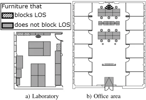
Fig. 1 shows the two different scenarios that we have mod-eled in our raytracer, that are part our research facilities. This allows us to compare the simulations with real measurement data. For both scenarios, for brevity we use discuss results for one specific Access Point (AP) placement, located in the upper
a) Laboratory b) Office area
Fig. 1: Evaluation Scenarios
part in both cases, as indicated in the figure. The AP is able to transmit at 1.8, 3.5, 28 and 61 GHz. Our measurements are done at a height of 1.65m. The gray areas on the map show the furniture that is below 1.65m, and therefore does not block LOS.
The first scenario, Fig. 1 a), is a laboratory. The walls on the top and on the right are made of wood, and the left and bottom wall are concrete. The left wall has also 5 windows. Due to its small dimensions, 6m wide, 8m long and 3m high, the laboratory scenario is comparatively rich in multipath even at HF. The multipath components have different characteristics depending on the material they reflect on.
The second scenario, Fig. 1 b), is an office area which is 15m wide, 19m long and 3m high. 12 offices surround the central part of the office area with glass walls, and the division between the offices is a thin wall of wood. This scenario has also some NLOS areas due to 4 columns in the main area and a dividing wall in the middle near the bottom.
C. Metrics
In both scenarios, simulations have been taken at measure-ment points that are spaced 20cm apart. We apply a power threshold of 100dB (receiver sensitivity) and a dynamic range threshold of 20dB (i.e., we allow only paths that within 20dB of the strongest path) and remove paths which do not meet those constraints. This reflects typical hardware constraints.
• Number of equal paths: Represents the number of paths
that are geometrically identical in LF and HF. The higher the number of equal paths, the better the correlation.
• Fraction of equal paths: Represents the fraction of LF
paths that are also found at HF, e.g., if only 5 LF paths arrive to a point but those same 5 HF paths arrive as well, we obtain a value of 1.
• Delay spread: We use the definition established in [16],
where the path delays are weighted by the power of each path.
• Angle spread: The angle spread is given by the maximum
Fraction of equal paths
(a) 1.8GHz and 28GHz (b) 1.8GHz and 61GHz (c) 3.5GHz and 28GHz (d) 3.5GHz and 61GHz
Fig. 2: Path study for the laboratory scenario
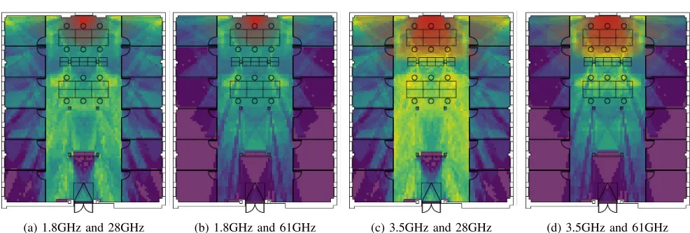
(a) 1.8GHz and 28GHz (b) 1.8GHz and 61GHz (c) 3.5GHz and 28GHz (d) 3.5GHz and 61GHz
Fig. 3: Path study for the office area scenario
paths in 3D. This gives a sense of directionality: the lower the spread, the more similar is the cluster of paths from the AP to that point.
• Angle profile correlation: The angle profile is a vector
that represents the power that arrives to a point for each arrival direction. We then correlate the angle profile of LF with the one of HF using the Pearson correlation coefficient.
D. Correlation of the actual channels
Fig. 2 shows the number of equal paths as well as the frac-tion of equal paths for the laboratory scenario. This scenario has a high number of equal paths, with more than 6 paths on average for each case. Near the AP there is a low number of equal paths, but the fraction is very high, i.e., those paths are typically available both at LF and HF. Due to the proximity to the AP, the direct path is very powerful and therefore most of the reflected paths are discarded due to the 20dB dynamic threshold. Common to all cases is also a diagonal stripe from the middle of the left wall to the bottom right corner. This stripe is caused by the column on the left wall, which blocks some of the reflections on that wall.
Regarding frequency behavior, we observe that 1.8GHz behaves quite similar compared to the two HF frequencies. The only noticeable difference is again the reflected stripe from the left column, which is higher attenuated at 61GHz.
As expected 3.5GHz behaves even more similar compared to HF, especially for 28GHz. In the latter case, the fraction of equal paths is close to 1 in most cases. Besides, the area near the AP that has a low number of equal paths is bigger for 3.5GHz than for 1.8GHz. This is because 3.5GHz has slightly fewer paths around that area compared to 1.8GHz due to the higher attenuation and the dynamic threshold, and this number of paths is closer to that of HF.
Fig. 3 illustrates the results of the path study for the office area scenario. This scenario is heavily influenced by NLOS, and this becomes clear from the difference between 28GHz and 61GHz. Although both of HF frequencies are significantly attenuated, the penetration of 28GHz through the glass walls of the offices is much better than that of 61GHz. 28GHz drops from 15-20 equal paths to 5-7, whereas 61GHz looses coverage in most of the cases. In the middle part of the scenario, the actual office area, the influence of the columns is noticeable and at 61GHz there is a visibly lower correlation behind the them. As in the laboratory scenario, the highest path fraction correlation is between 3.5GHz and 28GHz, this is again due to a similar attenuation between those frequencies.
0 5 10 15 20 25 Delay spread (ns) 0
0.2 0.4 0.6 0.8 1
CDF
1.8GHz 3.5GHz 28GHz 61GHz
(a) Delay spread
0 50 100 150 200 Angle (º)
0 0.2 0.4 0.6 0.8 1
CDF
1.8GHz 3.5GHz 28GHz 61GHz
(b) Angle spread
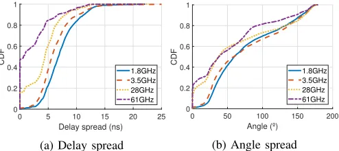
Fig. 4: CDFs for the office scenario
and reduction of multipath components due to attenuation. Comparing the two extreme cases, 1.8 GHz and 61GHz, only 20% of the positions present a delay spread lower than 5ns for the former, whereas this same delay value represents more than 80% of the points for the latter. In terms of similarity between delay spreads, once again, 3.5GHz and 28GHz show the closest behavior. Lastly, our results show that although number of paths, power per path and maximum delay spread are always higher for all measured points for LF, somewhat counterintuitively the winner metric delay spread can be higher for HF for almost 10% of the measured points. If the cluster of paths of LF close to the mean delay value is not present in HF, and only more distant paths are present with relatively close power values, delay spread can be higher after power normalization for HF.
Fig. 4b illustrates the CDF for the angle spread. On average, both LF frequencies have a higher angle spread than HF due to much stronger higher-order reflections. 61GHz has the lowest angle spread since it is the most attenuated frequency and, consequently, most reflections are lost. Also we can see that for LF the angles are evenly distributed, whereas for HF the points that are further away only receive the direct path.
The office area scenario can be divided into three main areas where DS and AS behave similarly. The LOS part in the middle area, usually presents the higher values of DS and AS, this holds true for all the frequencies. In the middle area, the values of DS quickly drop when there is a blockage, such as the pillars or the wall in the bottom half part, but since the scenario still holds its geometry on those points the AS is still high. The last area conforms the inside of the offices surrounding the middle area. This area has a higher values of DS similar to those in the Obstructed-Line Of Sight (OLOS) sections of the middle part, but the AS quickly lowers as the offices are further apart from the AP.
E. Correlation of the observed channels
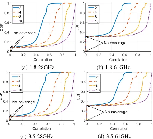
The previous simulation study investigated the actual corre-lation of the LF and HF channels. However, from a practical point of view, it is crucial to study the channels as they are perceived through the respective antennas. In particular, the number of antennas plays a vital role to differentiate paths in the spatial domain, as with N antennas we can theoretically differentiate up to N −1 paths. In addition, HF systems
typically have a larger number of antennas compared to LF, as the higher frequency allows for smaller antenna elements and thus a higher number of them can be inegrated in the same area. Therefore, the correlation is likely to improve when the number of antennas at LF is closer to the one at HF (for example for massive MIMO LF systems that incorporate a large number of antennas at the base station). For this reason, this section studies the minimum number of antennas at LF required to observe a meaningful correlation. We consider 16 antennas in HF (for both transmitter and receiver) and 2, 4, 8 and 16 antennas for LF at the receiver side. For simplicity we use an omnidirectional antenna for the transmitter.
We use the angle profile, i.e. the power associated with each angle, as a metric for the correlation to analyze not only the behavior of the reflection but also the losses. To estimate the angle profile, the channel at reception, h, given by the raytracer, is multiplied by the steering vector. We define the steering vector as
s(θ) = [1e−jπsin(θ).... e−jπ(N−1) sin(θ)], (1)
whereNis the number of antenna elements. Further, we define the channel as
h= [hoh1.... h(N−1)], (2)
wherehn is the channel coefficient for antennan. The angle profile (AP) is given by
AP =|s(θ)Hh| −π
2 ≤θ≤
π
2. (3)
The angle profiles are estimated for each measurement point in the open area for the frequencies of 3.5GHz and 61GHz and the results are illustrated in Fig. 5. For the case of 2 antennas at LF, the correlation is around 40%, dropping to 20% in the OLOS parts behind the pillars. The correlation quickly improves for 4 antennas at LF, averaging a 65% of correlation for the whole scenario but also dropping to 30% for OLOS. With 8 antennas, half of the antennas used for HF, the correlation goes up to 85% on LOS and around 50% on OLOS. When using 16 antennas at both LF and HF, the correlation over the whole scenario is around 90%. With this number of antennas, even in the OLOS part of the scenario the correlation is 80%, and even in NLOS, bottom middle part, the correlation goes up to 50%.
(a) 2 antennas at LF (b) 4 antennas at LF (c) 8 antennas at LF (d) 16 antennas at LF
Fig. 5: Antenna profile correlation for 3.5GHz and 61GHz
0 0.2 0.4 0.6 0.8 1
Correlation 0
0.2 0.4 0.6 0.8 1
CDF
2 4 8 16
No coverage
(a) 1.8-28GHz
0 0.2 0.4 0.6 0.8 1
Correlation 0
0.2 0.4 0.6 0.8 1
CDF
2 4 8 16
No coverage
(b) 1.8-61GHz
0 0.2 0.4 0.6 0.8 1
Correlation 0
0.2 0.4 0.6 0.8 1
CDF
2 4 8 16
No coverage
(c) 3.5-28GHz
0 0.2 0.4 0.6 0.8 1
Correlation 0
0.2 0.4 0.6 0.8 1
CDF
2 4 8 16
No coverage
(d) 3.5-61GHz
Fig. 6: CDFs for the antenna profile correlation for different numbers of LF antenna elements and 16 HF antennas
IV. PRACTICALVALIDATION
The aim of this section is to validate the LF and HF correlation through real-world measurements in the scenarios mentioned above. For brevity, we focus on the angle profile correlation metric for this section, because it encompasses the most important information. The equipment and the procedure used for the measurements are the following:
• LF: Our set up consists of a BladeRF SDR as transmitter with an omnidirectional antenna, and a USRP X310 equipped with TwinRX daughterboards connected to a 4 element antenna array, which is in line with current mobile systems. This setup ensures phase synchronization among antennas elements. We use the MUSIC pseudo-spectrum [17] to estimate the angle profile.
• HF: We transmit a pulse signal up-converted to the HF band with an up converter (SiversIMA) which operates
at 61.48GHz. The signal is transmitted by an omnidi-rectional antenna. On the receiver side, a horn antenna with an aperture of 7 degrees is used. Likewise, the horn antenna is connected to a SiversIMA operating at 61.48GHz. A motor rotates the set up by 360 degrees in steps of 4 degrees, resulting in the different steering directions. We build the angle profile by computing the received power at each step.
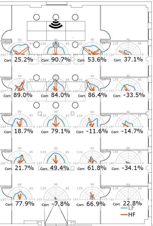
The measured angle profiles are illustrated in Fig. 7 and they were taken in the office scenario for the frequencies 3.5 and 61GHz. Values in the graph for HF range from -50dBm to -70dBm , with each concentric semicircle representing a step of -5dBm, whereas for LF they range from 0dBm to -20dBm. Due to the reduced number of antennas at LF, the angle profile is not fine-grained, and the system can not differentiate many paths. However, values for correlation between LF-HF angle profiles are generally high for points in LOS, with values between 65 and 91%. For the bottom row, and in particular behind the dividing wall, the low receive power makes it difficult to clearly identify the main path.
The third row from the top presents peculiar behavior due to a pillar obstructing LOS. The strongest path for LF is pointing to the wall, a reflection, whereas HF’s strongest path is obstructed LOS; this yields the lowest correlation values, around 15%. We observe similar behavior inside the offices, where received power is greatly attenuated. Inside the offices, LF generally finds reflections inside the room as the strongest path, and HF points to the AP but with low power. In these cases, correlation drops to values between 15% and 35%. Finally, we also took measurements with office doors closed, finding very low correlation and low power values for HF, with some coverage available only in the first two offices closest to the AP.
V. LF ASSISTEDBEAM-STEERING
Fig. 7: Angle profiles for LF and HF in the open area
power. Such an approach is time consuming: it takes20µs to check each sector and changing beam patterns takes around
1µs. To reduce the beam training overhead, we propose a system where the sector selection is performed by the angle profile information from LF. We check the sectors at HF according to the most powerful sectors of LF. For our results we take a fixed antenna width of5◦,10◦or20◦. We assess the system comparing the SNR loss of this approach to the optimal brute forcing as a function of number of sectors checked, i.e., a function of time devoted to beam training. We evaluate the system using both simulations and practical measurements. We use 4 antennas at LF and the pair of frequencies chosen are 3.5GHz and 61GHz.
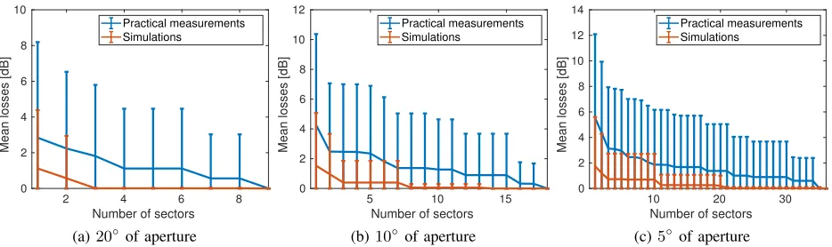
The results are illustrated in the error bar plot in Fig. 8. We illustrate the losses for the 20 measurement points used in the practical measurements. The middle point of the bar is the mean of the losses, the upper whiskers represents the 90% quantile and the lower whiskers the lowest value. Although for both cases, zero losses are the most frequent value, mean losses for practical measurements are around two times higher compared to the simulations, due to hardware imperfections and other real-world effects.
Regarding differences for the different sector widths, the losses follow a similar pattern as we use wider sectors. The losses in simulations for20◦HF sector width are 0.5dB when checking only 2 sectors around the best angle found at LF, which corresponds to40◦. With10◦ and5◦sectors, the losses are 0.5dB checking 3 and 11 sectors, corresponding to 30◦
and55◦ respectively. Contrarily to simulations, zero losses in the practical measurements are only reached when checking all the sectors, as there always exist very rare cases where the next direction is the last one to be checked. Overall, these results show that directly using the angle given by LF already gives a very good steering direction for HF. Further, there is a considerable reduction in SNR loss when checking only one or two additional sectors, meaning that the highest power values of HF are indeed generally within the two-three most powerful sectors at LF. As a consequence, we can reduce the overhead of the beamsteering process to one third of its original time with an average loss of only 2dB.
VI. CONCLUSIONS
In this work we study the correlation of different frequency bands. We show that cooperation between high frequency and low frequency in multiband systems can boost system perfor-mance. Our simulation results with a raytracer for an ideal scenario show that the pair of studied frequencies with the most similar behavior is 3.5 and 28GHz. We also investigate the effect of the number of antenna elements on the perceived correlation, showing that having 4 antennas at LF and 16 at HF already suffices to exploit correlation, and scaling up the number of LF antennas to 16 gives almost full correlation. Furthermore, we carry out hardware measurements at 3.5 and 61GHz to validate the simulations. We find that for a limited number of antennas at LF, 4, angle profiles have a high correlation between 70% and 90% for LOS, whereas for NLOS, the correlation drops to values between 15% and 30%. That means that even with a small number of antennas, the strongest paths at LF correspond to the strongest paths at HF for most of the cases.
Finally, we include an application of correlation by comput-ing what is the loss in power if the angle profile information of LF is directly applied to steer the antenna beam at HF, one of the most resource intensive procedures for mmWave systems. Results for simulations and practical measurements show we using a minimal set of sectors around the angles predicted by LF result in very low SNR loss, thus reducing the beamsteering overhead to one third of its original time with an average loss of less than 3dB.
REFERENCES
[1] (2016, Jul.) FCC adopts rules to facilitate next generation wireless technologies. [Online]. Available: https://www.fcc.gov/document/fcc-adopts-rules-facilitate-next-generation-wireless-technologies
[2] H. Xu, T. S. Rappaport, R. J. Boyle, and J. H. Schaffner, “Measurements and models for 38 GHz point-to-multipoint radiowave propagation,”
IEEE Journal on Selected Areas in Communications, vol. 18, no. 3,
pp. 310–321, March 2000.
2 4 6 8 Number of sectors 0
2 4 6 8 10
Mean losses [dB]
Practical measurements Simulations
(a)20◦ of aperture
5 10 15
Number of sectors
0 2 4 6 8 10 12
Mean losses [dB]
Practical measurements Simulations
(b)10◦of aperture
10 20 30
Number of sectors 0
2 4 6 8 10 12 14
Mean losses [dB]
Practical measurements Simulations
(c)5◦ of aperture
Fig. 8: Beam steering losses comparing to brute forcing
[4] P. Ky¨osti, I. Carton, A. Karstensen, W. Fan, and G. F. Pedersen, “Frequency dependency of channel parameters in urban los scenario for mmwave communications,” in10th European Conference on Antennas
and Propagation (EuCAP), 2016, pp. 1–5.
[5] A. O. Kaya, D. Calin, and H. Viswanathan, “28 GHz and 3.5 GHz wireless channels: Fading, delay and angular dispersion,” inIEEE Global
Communications Conference (GLOBECOM), 2016, pp. 1–7.
[6] A. Ali, N. Gonz´alez-Prelcic, and R. W. Heath, “Estimating millimeter wave channels using out-of-band measurements,” inInformation Theory
and Applications Workshop (ITA), 2016. IEEE, 2016, pp. 1–6.
[7] N. Gonzalez-Prelcic, A. Ali, V. Va, and R. W. Heath, “Millimeter-wave communication with out-of-band information,”IEEE Communications
Magazine, vol. 55, no. 12, pp. 140–146, DECEMBER 2017.
[8] T. Nitsche, A. B. Flores, E. W. Knightly, and J. Widmer, “Steering with eyes closed: mm-wave beam steering without in-band measurement,” in
IEEE Conference on Computer Communications (INFOCOM). IEEE,
2015, pp. 2416–2424.
[9] S. Sur, X. Zhang, P. Ramanathan, and R. Chandra, “Beamspy: Enabling robust 60 GHz links under blockage,” in Proceedings of the 13th Usenix Conference on Networked Systems Design
and Implementation, ser. NSDI’16. Berkeley, CA, USA:
USENIX Association, 2016, pp. 193–206. [Online]. Available: http://dl.acm.org/citation.cfm?id=2930611.2930625
[10] R. J. Weiler, M. Peter, T. Khne, M. Wisotzki, and W. Keusgen, “Simulta-neous millimeter-wave multi-band channel sounding in an urban access scenario,” in9th European Conference on Antennas and Propagation
(EuCAP), May 2015, pp. 1–5.
[11] G. Lovnes, J. J. Reis, and R. H. Raekken, “Channel sounding measure-ments at 59 GHz in city streets,” in5th IEEE International Symposium on Personal, Indoor and Mobile Radio Communications, Wireless
Net-works - Catching the Mobile Future., Sep 1994, pp. 496–500 vol.2.
[12] T. S. Rappaport, S. Sun, R. Mayzus, H. Zhao, Y. Azar, K. Wang, G. N. Wong, J. K. Schulz, M. Samimi, and F. Gutierrez, “Millimeter wave mobile communications for 5G cellular: It will work!” IEEE Access, vol. 1, pp. 335–349, 2013.
[13] J. Ryan, G. R. MacCartney, and T. S. Rappaport, “Indoor office wide-band penetration loss measurements at 73 GHz,” inIEEE International
Conference on Communications Workshops (ICC Workshops), May
2017, pp. 228–233.
[14] G. R. MacCartney, S. Deng, S. Sun, and T. S. Rappaport, “Millimeter-wave human blockage at 73 GHz with a simple double knife-edge diffraction model and extension for directional antennas,” inIEEE 84th
Vehicular Technology Conference (VTC-Fall), Sept 2016, pp. 1–6.
[15] H. Zhao, R. Mayzus, S. Sun, M. Samimi, J. K. Schulz, Y. Azar, K. Wang, G. N. Wong, F. Gutierrez, and T. S. Rappaport, “28 GHz millimeter wave cellular communication measurements for reflection and penetration loss in and around buildings in new york city,” inIEEE International
Conference on Communications (ICC), June 2013, pp. 5163–5167.
[16] P. Kysti, J. Meinil, L. Hentila, X. Zhao, T. Jms, C. Schneider, M. Narandzi’c, M. Milojevi’c, A. Hong, J. Ylitalo, V.-M. Holappa, M. Alatossava, R. Bultitude, Y. Jong, and T. Rautiainen, “IST-4-027756 WINNER II D1.1.2 v1.2 WINNER II channel models,” vol. 11, 02 2008. [17] H. L. Van Trees, Optimum array processing: Part IV of detection,