A statistical learning strategy for closed-loop control of fluid flows

Noname manuscript No.

(will be inserted by the editor)

A statistical learning strategy for closed-loop control

of fluid flows

Florimond Gu´eniat · Lionel Mathelin · M. Yousuff Hussaini

Received: date / Accepted: date

Abstract This work discusses a closed-loop control strategy for complex systems utilizing scarce and streaming data. A discrete embedding space is first built using hash functions applied to the sensor measurements from which a Markov process model is derived, approximating the complex system’s dynamics. A control strat-egy is then learned using reinforcement learning once rewards relevant with respect to the control objective are identified. This method is designed for experimental configurations, requiring no computations nor prior knowledge of the system, and enjoys intrinsic robustness. It is illustrated on two systems: the control of the tran-sitions of a Lorenz 63 dynamical system, and the control of the drag of a cylinder flow. The method is shown to perform well.

Keywords Closed-loop control, Reinforcement learning, Machine learning

1 Introduction

While the design and capability of aircraft, and more generally of complex sys-tems, have significantly improved over the years, closed-loop control can bring further improvement in terms of performance and robustness to non-modeled per-turbations. In the context of flow control, closed-loop control however suffers from severe limitations preventing its use in many situations. As a paradigmatic ex-ample, a typical turbulent flow involves both a large range of spatial scales and

Florimond Gu´eniat

Department of Mathematics, Florida State Univ.,

32306-4510 Tallahassee, FL, USA E-mail: [email protected]

Lionel Mathelin

LIMSI-CNRS, rue J. von Neumann, Campus Universitaire d’Orsay, 91405 Orsay cedex, France

M. Yousuff Hussaini Department of Mathematics, Florida State Univ.,

exhibits a rich and fast dynamics. High frequency phenomena hence require a con-trol command fast enough to adjust to the current state of the quickly evolving flow system. Indeed, frequencies of interest can routinely lie over 1 kHz, leading to a very short period of time for the controller to synthesize the command based on its knowledge of the state of the system.

While flow manipulation and open-loop control are common practice, much fewer successful closed-loop control efforts are reported in the literature. Further, many of them rely on unrealistic assumptions. For example, Model Predictive Control (MPC) approaches require very significant computational resources to solve the governing equations in real-time. If a Reduced-Order Model (ROM) is employed, as is common practice to alleviate the CPU burden, one often needs to observe the whole system for deriving the ROM as, for instance, the velocity or pressure fields with Proper Orthogonal Decomposition (POD), see [1–6]. Hence, flow control with this class of approaches is restricted to numerical simulations or experiments in a wind tunnel equipped with sophisticated visualization tools such as Particle Image Velocimetry (PIV).

This paper discusses a practical strategy for closed-loop control of complex flows by alleviating the limitations of current methods. The present work relies on a change of paradigm: we want to derive a general nonlinear closed-loop flow control methodology suitable foractual configurations and as realistic as possible. No a priori model, nor even a model structure, describing the dynamics of the system is required to be available. The approach proposed isdata-driven only, with the sole information about the system given by scarce and spatially-constrained sensors. The method then exploits statistical learning methods.

This is the framework one typically deals with in practical situations where the amount of information on the system at hand is limited and usually comes from a few sensors located at the boundary of the fluid domain,e.g., on solid surfaces. The resulting information takes the form of short time-dependent vectors with as many entries as sensors.

Among the few earlier efforts relying on streaming measurements from a few sensors, a trained neural network using surface measurements is employed to re-duce the drag of a turbulent channel flow with an opposition control strategy in [7]. In [8], pressure sensors and an auto-regressive model (AutoRegression with eXoge-nous inputs, ARX) are used to reduce flow-induced cavity tones. An autoregressive approach is also followed in [9] and [10], while a genetic programming technique is adopted in [11] to control a separated boundary layer. Interested readers may refer to [12] for a comprehensive review of the topic. The present approach aims at deriving an efficient, yet robust, nonlinear closed-loop control method compliant with actual situations. Among its distinctive features compared to other methods is a combination ofbothperformance and fast learning.

dynamics allows the derivation of a reinforcement learning-based control strategy of the identified Markov process model of the system. The control of Markov processes is a mature field, [15] and reinforcement learning, [16, 17], is a suitable class of methods for the control of Markov processes, see for instance [18, 19] for the control of 1-D and 2-D chaotic maps. As will be seen in the application examples below, the resulting control strategy is data-driven only, intrinsically robust against perturbations in the flow and does not require significant computational resources nor prior knowledge of the flow. The proposed approach is experiment-oriented and on-going efforts are carried-out to demonstrate it on an experimental open cavity flow in a turbulent regime. This will be the subject of a subsequent publication.

The paper is organized as follows. The framework and basics of how hash func-tions are used to generate a low-dimensional state space are discussed in Section 2. Section 3 is concerned with learning an efficient control strategy for the system modeled as a stochastic process living in a small dimensional space. The resulting control strategy is illustrated and discussed in the case of the control of a Lorenz 63 system and the drag reduction of a cylinder in a two-dimensional flow in Section 4. Concluding remarks close the paper in Section 5.

2 Hash functions for reduced order modeling

2.1 Preliminaries

Consider a dynamical system evolving on a manifoldD: ˙

X(t) =f(X(t)), X∈ D,

with X the state of the system and fthe flow operator. Let g : D → _Rnp _{be a}

sensor function. In the sequel, the number of sensorsnpwill be taken to be one but

generalization to more sensors is immediate. The observed datay ∈_R is defined asy(t) :=g(X(t)).

Let ∆t be the sampling rate of the measurement system. Sampling has to be fast enough to capture the small time scales of the dynamics ofy. The data coming from the sensor are embedded in a reconstructed phase spaceΩ:

(y(t)y(t−∆t). . . y(t−(ne−1)∆t)) =:y(t)∈Ω⊂Rne.

The correlation dimension ofy is estimated from the time-series, for instance using the Grassberger-Proccacia algorithm, [20]. It allows the definition of the embedding dimensionneas, at least, twice the correlation dimension. Under mild

assumptions, this resulting embedding dimension ensures there is a diffeomorphism between the phase spaceD and the reconstructed phase space, [21], so thaty is an observable on the system.

2.2 Hash functions

A hash function is any function that can be used to map an entry y ∈ _Rne _to

two different entries so that slightly different input data should result in a large variation of the associated key, [22]. An important objective in choosing the hash function is to avoidcollisions,i.e., when two different entries are associated with the same key.

Conversely, the need for identification of similar entries in large databases has led to the use of the Locality-Sensitive Hash functions (LSH) [23, 13]. In contrast with most hash functions, they are designed to promote collisions when two entries are close to each other. The idea is that, if two points are close inRne, they should be likely to remain close after a projection on a lower dimensional subspace. The Johnson-Lindenstrauss lemma (JLL), [24], provides useful results to reach this objective and motivates the use of LSHs. Specifically, the JLL provides proba-bilistic guarantees of the near preservation of relative distances between objects in high-dimension after projection onto random low-dimensional spaces.

Let v ∈_Rne_{, kvk}

2 = 1, be a test vector. The function h

v,w _:

Rne →N is a LSH, [23]:

hv,w(y) :=h0+

jv·y w

k

, (1)

where b·cis the floor operator, w >0 a quantization length and h0 is such that

hv,w >0,∀y∈Ω,v∈Bne

2 (1), with B

ne

2 (1) the unit ball ofR

ne _{in the sense of} L2. As an illustration, following [24, 13], if two observablesy₁ and y₂ are such thatky1−y2k2 < r, withr= w/2kvk2, they are associated with the same key

with a probabilityp1 larger than 1/2. On the other hand, the probabilityp2 that

two distant pointsy₁ andy₂ appear close to each other in the sense ofhv,wis a function of the angle between (y₂−y₁) andv and is smaller thanp1.

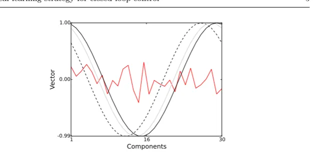
Let us illustrate the LSH with a simple example. Let ne= 30 andya,yb and ycbe three vectors fromRne such that:

yaj = cos (2π (j−1)), 1≤j≤ne,

ybj = cos (2π (j)),

ycj = cos (2π (j+ 2)).

Let v be a unit-norm normal Gaussian vector of Rne,w = 0.2 and h0 = 0. The

different vectors are drawn in Fig. 1. Upon processing with the LSH, the keys associated with the three vectorsya,yb andycare:

hv,w(ya) = 3, hv,wyb= 3, hv,w(yc) = 1.

ya andyb are closer to each other, in the sense of theirL2-distance, than toyc, and indeed, vectorsyaandyb are associated with the same keys= 3 whileycis associated withs= 1.

To discriminate false neighbors with higher probability, projections on several low-dimensional subspaces can be used. Consider the hash functionh:Rne → S ⊂ N made of concatenation of nv keys {hvl,wl(y)}n_l=1v . Many choices can be made

for the test vectors {vl}l. For instance, they could be the principal axes of the

manifold on which the observable y evolves, or may be randomly selected from a Gaussian distribution. Keys (i.e., objects in the image space of h) generate a Vorono¨ı paving of the observable space. Each key is associated with a cell, orstate

s, and close observables are associated with the same key.

Coarseness of the paving depends on the quantization lengths {wl}l and the

1 16 30 Components

-0.99 0.00 1.00

Ve

cto

r

Fig. 1 Plot of the vectorsya_andyb_{(solid lines) andy}c_{(dashed line). The random test vector} vis plotted in red.

cells1 and, as wl increases, the cardinality nkey := card (S) of the image space

of h decreases. On the other hand, increasing nv is equivalent to refining the

description,i.e., increasing the cardinality ofS.

3 State-driven control

Thanks to the hash function, the original infinite-dimensional system is approxi-mated as a discrete stochastic process whose state space is spanned by the keys. The system is observable in real-time in this discrete space since evaluating the hash function with the streaming sensor datay can be done at no computational cost. Under a discrete control commanda∈ A to the actuators, hereafter termed the action, the dynamics of the system will be modified and the goal is to find the action which makes the physical system at hand satisfy the control objective, say, a target dynamics. The discretized description of the system with the hash function naturally lends itself to a Markovian framework, [25, 26], which is adopted below.

3.1 Markov Decision Process

Let p(i, l, j) be the probability of transition from a state s(i) ∈ S to s(j) ∈ S under an action a(l) ∈ A, A := na(l)∈_R, l∈ IA:= [1, na]⊂N

o

being a uni-formly discretized space of possible control actions. Here again, the analysis is restricted to one actuator but generalization to more actuators is immediate. Actions

n a(l)

ona

l=1 index the discrete commands available to the controller.

De-fineS :=

n

s(i), i∈ IS:= [1, nkey]⊂N

o

andsk ≡ s(tk:=k ∆t). Similarly,ak ≡

a(tk). To each transition-action (i→j, l) is associated atransition reward (TR)

1 _{Two vectorsy}

1 andy2 are associated with two different keys if theirL2-norms differ by

R

s(i), a(l), s(j)

2_{. The goal of the control strategy is hence to identify the}

opti-malpolicy π :S → A, which describes the best action to apply when in a given state so as to maximize thevalue, Viπ, defined as the sum of the future expected

rewards of the policy when starting at states(i):

Viπ := lim

K→∞E

" _K X

k=1

γk−1R(sk, π(sk), sk+1)

#

, s1=s(i), (2)

whereE[·] is the expectation operator over all possible sequences{sk}Kk=1 under

the policy π. Here, γ is the discount rate, 0< γ <1. By weakly accounting for TRs occurring far in the future, the discounted rate effectively introduces a time horizon. The values express the expectation of the cumulative TRs of a given policy. Eq. (2) may be reformulated as, [15]:

Viπ=R π

i +γ

X

j∈S

p(i, πs(i), j)Vjπ, (3)

where Rπi := E

h

Rsk=s(i), π(sk), sk+1

i

is the mean TR in state sk = s(i)

under the policy π. This corresponds to the celebrated Bellman equation, [27], written in the discrete settings.

3.2 Identification of the rewards

The transition rewards are unknowna prioriand depend on the control objective. As perhaps more familiar to the reader, one could define the cost as the opposite of the reward. Consequently, to learn relevant rewards, consider the cost function J associated with the control objective:

J(tn) :=

∞ X

k=0

γkC(tn+k+1) +ρ|a(tn+k)|2

, (4)

with C the measure of performance, e.g., the drag coefficient in the included ex-ample. The contribution of the control intensity |a|2 to the cost with respect to the measure of performanceC is weighted byρ >0.

Let the immediate rewards Rimm(sn, an, sn+1) represent, at any given time

tn, the negative of the contribution to the costJ(tn) of the transition from the

present statesn≡s(tn) to statesn+1, under an action an≡a(tn):

Rimm(sn, an, sn+1) :=−

C(tn+1) +ρ|a(tn)|2

. (5)

Rimm is then high when the performance associated with the controlled system

is good, and low otherwise. Instead of the reward associated with a particular tra-jectory in the original, infinite-dimensional, phase space, theaverage, trajectory-independent, reward associated with all trajectories leading to a given transition (sn→sn+1, an) should be determined. The ergodicity assumption postulates the

2 _{We use a slight abuse of notation as we consider R s}(i)_{, a}(l)_{, s}(j)

≡ R(i, l, j) and

p i, a(l)_{, j}

equivalence of a temporal and an ensemble average,i.e., here lim

K→∞K

−1

K−1

X

k=0

f(sk) =E[f(s)]. Under this assumption, the mean transition rewards, in the sense of the probability

distribution ofRimm, are finally determined during the learning stagevia:

R(sn, an, sn+1)←(1−αn)R(sn, an, sn+1)

| {z }

old value

+αnRimm(sn, an, sn+1), (6)

with αn > 0 the learning rate. For the TRs to be associated with the average

contribution to the cost function of the transition-action (sn→sn+1, an), the

learning rate is set to αn = 1/N(i,l,j), where N(i,l,j) ∈ N corresponds to the number of times the transition-action

s(i)→s(j), a(l)

has occurred so far during the learning process.

3.3 Reinforcement learning

To derive a control strategy, one needs to determine a policy which would give the best control action given the current state of the system, as known through the hash function. The rewards associated with an action when in a given state have been learned and this information is now used to derive a control policy to drive the system along transitions and actions associated with the largest rewards.

When the probabilities of transition from a state to another are known, the policy may be identified by means of a dynamic programming algorithm, [27, 15]. However, the distribution of transition probabilities and values{Viπ}i∈IS are

difficult to reliably evaluate since neither the control policy nor the transition probabilities are stationary during the learning stage. In this situation, Reinforce-ment Learning is a suitable class of methods for the control of Markov processes, [16, 28, 29].

Among these methods, the Q-learning approach consists in relying on the estimation of the Q-factors, or action-values, Qπ which evaluate the expected reward of a state-action combination:

Qπ(i, l) :=DRi

a(l)E+γ X

j∈S

p(i, π(i), j)Vjπ, (7)

where

D Ri

a(l)

E

:=E

h R

sk=s(i), a(l), sk+1

i

is the empirical mean TR as-sociated with applying the action a(l) when in the state s(i). From Eq. (3), the action-value is hence the expected average reward of applyinga(l) while in state

s(i)and subsequently following the policyπ.

As stated previously, the transition probabilities can not be accurately esti-mated. However, an iterative estimation of the Q-factors can be derived, [16, 29, 17]. Letting the initial Q-factors be given, the Q-factor associated with a states(i)

Qπ(i, l)←Qπ(i, l)

| {z }

old value

+αn∆Qπ, (8)

∆Qπ :=



    R

sn=s(i), a(l), sn+1

+γmax el∈IA

Qπ

i,el

| {z }

“best” value

−Qπ(i, l)

| {z }

old value



    ,

whereαn>0 is a learning factor. It can be shown thatQπ converges to the true

Q-factors when n → ∞ if the following conditions hold, [16]: i) the TRs R are bounded,ii)0< αn<1,∀n∈N,iii)

∞ P

n=1

αn→ ∞andiv)

∞ P

n=1

(αn)2<∞.

The action-valueQπ(i, l) will increase when the reward associated with the 2-tuples(i), a(l)is good,i.e., such that∆Qπ >0, and decrease otherwise. To learn a good policy, the system in different states is stimulated with different actions to estimate the Q-factors. The control policy is the action which, for each state, is associated with the largest Q-factor, [16, 29].

3.4 Robustness

A critical property of any realistic and practically useful control strategy is its resilience with respect to unpredictable events. These events encompass exoge-nous/external perturbations to the flow, sensor noise, actuator noise, etc. A control strategy robust to these perturbations is passive and brings the flow back to its nominal controlled state after the perturbation is gone. As will be demonstrated in the application example below, see section 4.2.3, the present strategy is robust thanks to two properties:

First, the state of the system, as estimated via the LSH, is discrete. The locality sensitivity property of LSHs implies that a small perturbation of the measure-ment vectory will likely result in the same key as the unperturbed measurement,

hv,w(y+) =hv,w(y). More precisely, the state estimation is strictly robust to any perturbation of energykk₂with probability

nv Y

l=1

max0,1− kk₂|cos (∠(,vl))|/w

.

4 Results

4.1 Dynamical system

To illustrate the methodology discussed above, we now consider the Lorenz 63 system [30], defined by the following equations:

     

    

dX1

dt =σ(X2−X1) +fX1(X, t)

dX2

dt =X1(r−X3)−X2+fX2(X, t)

dX3

dt =X1×X2−bX3+fX3(X, t),

(9)

with the common parameters (σ, r, b) = (10,20,8/3). A chaotic attractor defines the dynamics, structured as two “wings” around two fixed points of the sys-tem. The state vector evolves on a wing, turning around a fixed point, before eventually jumping to the other wing. fXi is the action on the component i of

X := (X1X2X3). The chosen control objective is to remain on the “left” wing,

X1 ≤ 0. The measure of the performance is given as the distance between the

state vector and the left fixed point X? of the system, C := kX−X?k₂, with

X?:=

−p

b(r−1),−p

b(r−1), r−1

.

The observabley is constructed from the time series{y(t−n ∆t)}ne−1

n=0 ofX2,

sampled every∆t= 0.025 time units. In this illustration, onlyfX1is different from

zero so that the Lorenz system is controlled only through the time-derivative dX1/

dt of the first component of its state vector. It mimics a realistic scenario, where sensors and actuators are distinct. Actuation values lie between [−26,26] with a discretization step of 4. This leads tona = 14 different actuations to control the

system. The cost function to minimize is given by Eq. (4) and the control command is penalized withρ= 0.1.

The embedding dimension is set to ne= 8. The first three singular vectors of

ane×N Hankel matrix, built onN= 500 measures{y(t−n ∆t)}N_n=0−1, are used

as thenv = 3 test vectors{vl}nl=1v of the LSHs. The quantization length is set to

w= 45 and leads to a cardinality of the set of keys ofnkey= 14.

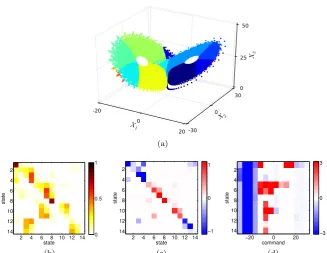
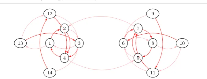
Once the test vectors are determined from the Hankel matrix, the states are to be identified via the LSHs, see Fig. 2(a). It is hence possible to infer both the dynamics of the system from the state transitions and the rewards associated with the objective. The mean transition probabilities from one state to another, after five time increments in order to improve visualization, are plotted in Fig. 2(b). As expected for the Lorenz system, the dynamics are seen to be driven by two main cycles, see Fig. 4. There are two statistically dominant sequences of transitions cycling around all states between 1 (resp. 5) and 4 (resp. 8), corresponding to the right (resp. left) wing of the Lorenz attractor. States 9 to 11 and 12 to 14 represent sub-transitions from a main cluster to another one.

From the observations of the system, one learns the nkey×na×nkey'2100

transition rewards matrixRand thenkey×na'150 Q-factors matrixQby

X₁ -20

0

20

X2

-30 0

30 X3

0 25

50

(a)

state

state

2 4 6 8 10 12 14 2

4 6 8 10 12 14

0 0.5 1

(b)

state

state

2 4 6 8 10 12 14 2

4

6

8

10

12

14 −1

0 1

(c)

command

state

−20 0 20

2

4

6

8

10

12

14

−3 0 3

(d)

Fig. 2 (a): Identified clusters (color-coded) for the Lorenz 63 system. (b): Mean state tran-sition probabilities. The trantran-sition matrix has been iterated five times for readability. (c): Transition rewards associated with a state transition, for the NULL command. The TRs have been rescaled between−2 and 2 and the colormap saturated, in order to improve readability. (d): Q-factors.

−20 0 20 −50

050 0

25 50

X

2

X

1 X3

(a)

time

component X

1

0 10 20 30

−20 −10 0 10 20

(b)

Fig. 3 Uncontrolled Lorenz system in dashed black. Controlled response in solid red. The

identified strategy is applied at timet= 15. (a): State phase. (b):X1 component.

1 2

3

4

6 7

8

5 9

10

11 12

13

14 1

2

3

4

6 7

8

5 9

10

11 12

13

14

Fig. 4 Transitions between clusters for the Lorenz system. Only the first two most probable transitions are represented. The dark red arrows represent the most probable transitions from one cluster to another, while the pale red represents the second most probable transitions.

4.2 Two-dimensional numerical flow

To further illustrate the methodology discussed above, consider a 2-D laminar flow around a circular cylinder, in two situations: a fixed, or random in time angle of the incoming flow.

4.2.1 Configuration of the test case

The considered Reynolds number of the flow isRe = 200 based on the cylinder diameter and the upstream flow velocity. Details of the simulation can be found in [31]. The observabley is constructed from the time series{y(t−n ∆t)}n_ne−₌₀1 of a single pressure sensor, sampled every∆t= 0.75 time units. This sensor is located on the cylinder surface at an angle of 160 degrees from the upstream stagnation point when the angle is fixed. In this case, the pressure signal oscillates with a period of about 9 time units and half as much for the drag.

Actuation,i.e., control of the flow is achieved via blowing or suction through the whole cylinder surface. Actuation values lie within [−0.2,0.02], with a dis-cretization step of 0.02, ranging from suction to blowing. It leads to na = 12

different actuations to control the system. The cost function to minimize is given in Eq. (4), with ρ = 23. It corresponds to the drag (C is the drag coefficient) induced by the cylinder penalized with the intensity of the command. The penalty

ρwas chosen so that the resulting command remains within the operating range of the actuator. The embedding dimension is set tone= 14. The first five singular

vectors of ane×NHankel matrix, built onN= 500 measures{y(t−n ∆t)}N_n=0−1,

are used as thenv= 5 test vectors{vl}nl=1v of the LSHs. The quantization length

is set tow= 50 and leads to a cardinality of the set of keys ofnkey= 15.

action a

R

(3

4

,a

)

−0.2 −0.1 0

−2

−1.5

−1

−0.5

(a)

time

in

ci

d

en

t

a

n

g

le

0 30 60

−15 0 15

(b)

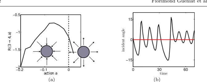
Fig. 5 (a): Transition rewards associated to the transition 3→4, with respect to the com-mand. The TRs have been rescaled between−2 and 2. The drawings illustrate the actuation (suction or blowing). (b): Time-evolution of the incident angle of the incoming flow, for the noiseless (red) and noisy (black) case.

4.2.2 Noiseless case: nominal incidence

Once the test vectors are determined from the Hankel matrix, and the states are identified viah, it is possible to infer the dynamics of the system and the associated rewards. The learned transition reward R3, a(l),4 is plotted in Fig. 5(a). It clearly exhibits a maximum which corresponds to the best compromise between a sufficient decrease ofCwhile a reasonable increase of|a|2_{. The estimated transition}

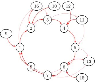
probabilities from one state to another are plotted in Fig. 6(a). In the present case, the dynamics are seen to be rather periodic, with a statistically dominant sequence of transitions cycling around all states between 1 and 8, see Fig. 7. Other states are “transient” states between two stages of the main cycle. For instance, a transition from state 1 to state 16 can occur with a low probability but the next transition will be to state 2 (or, less likely, state 3). Further analysis of the transition matrix can give more insights into the dynamics and on the relevance of other sequences, e.g., via stability analysis, [14], symbolic dynamics based on keys, [32], or the Kullback-Leibler entropy, [14].

From the observations of the system, one learns the nkey×na×nkey'2700

transition rewards matrix R and the nkey×na ' 180 Q-factors matrix Q by

repeatedly applying Eq. (6) and Eq. (9). As in the Lorenz system case (see above in Sec. 4.1), the transition matrix is sparse, as can be appreciated from Fig. 6(a), and many transitions hence hardly ever occur. Thus, the learned TRs and the Q-factors matrices are also sparse, see Fig. 6(b) and Fig. 6(c).

The performance of the control strategy is assessed in terms of the performance indicatorηdefined as the difference between the time-averaged costhJ i:=hJ(t)i_t and the time-averaged cost with a NULL strategy (a = 0), hJNULLi. The

perfor-mance indicator is scaled with the difference betweenhJNULLiand the costhJORAi

of an optimal time-invariant control strategy:

η:= (hJNULLi − hJ i)/(hJNULLi − hJORAi). (10)

The evolution ofη as a function of the learning effort, defined as the number

state s t a t e

5 10 15

5 10 15 0 0.5 1 (a) state s t a t e

5 10 15

5 10 15 −1 0 1 (b) command s t a t e

−0.2 −0.1 0

5 10 15 −1 0 1 (c)

Fig. 6 (a): Mean state transition probabilities. (b): Transition rewards associated with a state transition, for the NULL command. The TRs have been rescaled between−2 and 2 and the colormap saturated, in order to improve readability. (c): Q-factors.

1 2 3 4 5 6 7 8 9 10 11 12 13 15 16 1 2 3 4 5 6 7 8 9 10 11 12 13 15 16

Fig. 7 Transitions between clusters for the cylinder flow. Only the first two most probable transitions are represented. The dark red arrows represent the most probable transitions from a cluster to another one, while the pale red represents the second most probable transitions.

the learning stage focuses onto a limited number of unknowns and the Q-factors quickly converge.

As expected, the values {Viπ}i∈IS, computed with the learned policies are

larger than the values computed with theORApolicy, on average, see Tab. 1.

Policy NULL ORA Present strategy

Average valuehVπi -15.8 9.5 13.2

Table 1 Average expected valuehVπ_i:=

Ei∈IS

Vπ i

associated with the NULL, ORA and present strategy policies. The learning effort for the rewards (resp. the Q-factors) was 10000.

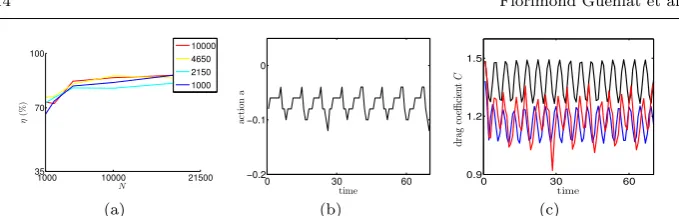
The resulting control command is plotted in Fig. 8(b) and is seen to exhibit an oscillatory behavior. The associated drag coefficient of the cylinder flow is plotted in Fig. 8(c) for the present approach as well theNULLand theORAstrategy. The identified control is seen to perform well. The drag coefficient for the identified control resembles the one given by theORAcontrol.

N

η

(%

)

1000 10000 21500

35 70 100

10000

4650

2150

1000

(a)

time

a

c

t

io

n

a

0 30 60

−0.2 −0.1 0

(b) (c)

Fig. 8 Illustration of the control policy. (a): Performance indicator with respect to the learning effort of the transition rewards matrixR. Colors (from blue to red) encode different efforts in learningQ. (b): Actuation as a function of time,a(t). (c): Time-evolution of the drag coefficient under three different control policies: zero command (NULL, black), ORA strategy (blue), and the optimal policy from the present approach (red).

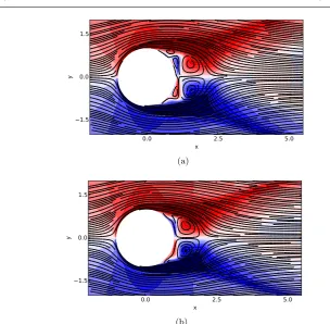
When control is applied, the pressure difference between the upstream stagnation point and the rear cylinder vicinity is significantly reduced. Further insights about the control effect can be gained by examining Fig. 10 where the time-averaged streamlines are plotted. With control,i.e., with a negative normal velocity at the cylinder surface, small recirculation bubbles significantly weaken, or even vanish, and the separation of the boundary layer from the cylinder surface is postponed further downstream, reducing the effective width of the wake. The length Lr of

the recirculation bubble drops fromLr= 1.11 in the case of theNULLcommand

(no control), see Fig. 9(a), to Lr = 0.95 when the command identified by the

present control approach is applied, see Fig. 9(b). The length of the recirculation bubble is hence reduced by 15%. Suction at the cylinder surface tends to slightly increase the viscous drag (thinner boundary layers with larger velocity gradients) but significantly decreases the width of the wake and the pressure defect at the back of the cylinder, producing a lower drag.

4.2.3 Measurements with noise

To investigate the robustness of our control strategy, the angle of the incident flow is made to vary randomly between −20 and 20 degrees around its nominal value with a uniform probability distribution and a smooth time-evolution, see Fig. 5(b) for a typical realization. This mimics a typical class of perturbations to the system at hand and allows the determination of the robustness of the control strategy.

As in the noiseless case considered in Sec. 4.2.2 above, the transition probabil-ity, rewards and Q-factors matrices are all sparse (not shown for sake of brevity). The performance indicatorηof the derived policy is depicted in Fig. 11(a). In con-trast with the noiseless case,ηis here strongly dependent on the effort in learning. At early stages of the learning process, the influence of the noise is prominent and the dynamics are not properly captured, which ultimately leads to poor control strategies.

Similarly as in Sec. 4.2.2, the values {Viπ}i∈IS, computed from the

0.0 2.5 5.0 x

−1.5 0.0 1.5

y

−2 −1 0

(a)

0.0 2.5 5.0

x −1.5

0.0 1.5

y

−2 −1 0

(b)

Fig. 9 Mean pressure field. (a): for the NULL command. (b): for the present identified control strategy. Note that only a part of the computational domain is plotted.

Policy NULL ORA Present strategy

Average valuehVπ_{i -6.8 3.0 8.0}

Table 2 Average expected valuehVπ_i:=

Ei∈IS

Vπ i

associated with the NULL, ORA and present strategy policies. The learning effort for the rewards (resp. the Q-factors) was 10000.

The associated drag coefficient of the cylinder flow is plotted in Fig. 11(c) for the present approach as well the NULL and the ORA strategy. Again, the identified control is seen to perform well and resembles that given byORA.

5 Concluding remarks

0.0 2.5 5.0 x

−1.5 0.0 1.5

y

(a)

0.0 2.5 5.0

x −1.5

0.0 1.5

y

(b)

Fig. 10 Vorticity field and streamlines for the mean field. (a): for the NULL command. (b): for the present identified control strategy. Note that only a part of the computational domain is plotted. Colors encode the sign of the vorticity.

N

η

(%

)

1000 10000 21500

35 70

100 10000

4650

2150

1000

(a)

time

a

c

t

io

n

a

0 30 60

−0.2 −0.1 0

(b) (c)

Fig. 11 Illustration of the control policy. (a): Performance indicator with respect to the

learning effort of the transition rewards matrixR. Colors (from blue to red) encode different efforts in learningQ. (b): Actuation as a function of time,a(t). (c): Time-evolution of the drag coefficient under three different control policies: zero command (NULL, black), ORA strategy (blue), and the optimal policy from the present approach (red).

are directly related to the control objective and tend to sort state transitions based on their impact on the control cost function. A reinforcement learning algorithm is then used to derive the optimal control policy, promoting transitions associated with good rewards.

functions and effective state-aggregation in a discrete phase space, the method runs in real-time and allows closed-loop control. Its discrete and ensemble-averaged na-ture also brings intrinsic robustness against perturbations in the flow.

This approach has been illustrated on two test cases. The control of a Lorenz system is achieved, by measuring only one component. To mimic a realistic sce-nario, the actuation is done on a different component. The method is also illus-trated by the two-dimensional flow around a circular cylinder. Measurements were provided by a single wall-mounted pressure sensor and actuation was achieved by blowing or suction of fluid at the cylinder surface. The drag coefficient was signif-icantly reduced, reaching essentially the same performance as the control policy given by theORAstrategy.

More generally, the method presented in this work is readily applicable to physical systems with a causal link between the actuators and the cost functional as evaluated from the sensors. It does not rely on a prior model and instead learns directly from observing the system under stimulation by the actuators, hence being suitable for practical configurations. An identified limitation of the proposed approach is the number of keys one needs to consider if the relevant dynamics of the system is very rich (largenkey) and/or a very fine control law is

required (largena). In this situation, the number of entries of theQmatrix grows

and hence possibly requires more data for learning. Approximation techniques have however been used to alleviate this limitation [33].

Current efforts concern the experimental control of the turbulent flow over an open cavity using the present approach and will be the subject of a subsequent publication. Further developments focus on the convolution kernels, an improved evaluation of suitable rewards and milder assumptions for the reinforcement learn-ing of the control policy.

References

1. J. Gerhard, M. Pastoor, R. King, B.R. Noack, A. Dillmann, M. Morzynski, and G. Tadmor. Model-based control of vortex shedding using low-dimensional galerkin models.AIAA J., 4262(2003):115–173, 2003.

2. M. Bergmann and L. Cordier. Optimal control of the cylinder wake in the laminar regime by trust-region methods and pod reduced-order models. J. Comp. Phys., 227(16):7813– 7840, 2008.

3. Z. Ma, S. Ahuja, and C.W. Rowley. Reduced-order models for control of fluids using the eigensystem realization algorithm.Theo. Comp. Fluid Dyn., 25(1-4):233–247, 2011. 4. W.T. Joe, T. Colonius, and D.G. MacMynowski. Feedback control of vortex shedding

from an inclined flat plate.Theo. Comp. Fluid Dyn., 25(1-4):221–232, 2011.

5. L. Mathelin, L. Pastur, and O. Le Maˆıtre. A compressed-sensing approach for closed-loop optimal control of nonlinear systems.Theo. Comp. Fluid Dyn., 26(1-4):319–337, 2012. 6. L. Cordier, B.R. Noack, G. Tissot, G. Lehnasch, J. Delville, M. Balajewicz, G. Daviller,

and R.K. Niven. Identification strategies for model-based control.Exp. Fluids, 54(8):1–21, 2013.

7. C. Lee, J. Kim, D. Babcock, and R. Goodman. Application of neural networks to turbu-lence control for drag reduction.Phys. Fluids, 9(6):1740–1747, 1997.

8. M.A. Kegerise, R.H. Cambell, and L.N. Cattafesta. Real time feedback control of flow-induced cavity tones - part 2: Adaptive control.J. Sound Vib., 307:924–940, 2007. 9. S.-C. Huang and J. Kim. Control and system identification of a separated flow. Phys.

Fluids, 20(10):101509, 2008.

11. N. Gautier, J.-L. Aider, T. Duriez, B.R. Noack, M. Segond, and M.W. Abel. Closed-loop separation control using machine learning.J. Fluid Mech., 770:442–457, 2015.

12. S. Brunton and B. Noack. Closed-loop turbulence control: Progress and challenges. App. Mech. Rev., 67(5):050801, 2015.

13. M. Slaney and M. Casey. Locality-sensitive hashing for finding nearest neighbors [lecture notes].IEEE Signal Process. Mag., 25(2):128–131, 2008.

14. E. Kaiser, B.R. Noack, L. Cordier, A. Spohn, M. Segond, M. Abel, G. Daviller, J. ¨Osth, S. Krajnovi´c, and R.K. Niven. Cluster-based reduced-order modelling of a mixing layer.

J. Fluid Mech., 754:365–414, 9 2014.

15. P. Mandl. Estimation and control in markov chains. Adv. App. Probab., pages 40–60, 1974.

16. C. Watkins and P. Dayan. Q-learning. Mach. Learn., 8(3-4):279–292, 1992.

17. A. Gosavi. Target-sensitive control of markov and semi-markov processes.Int. J. Control Autom., 9(5):941–951, 2011.

18. C.T. Lin and C.P. Jou. Controlling chaos by ga-based reinforcement learning neural network.IEEE T. Neural Networ., 10(4):846–859, 1999.

19. S. Gadaleta and G. Dangelmayr. Optimal chaos control through reinforcement learning.

Chaos, 9(3):775–788, 1999.

20. P. Grassberger and I. Procaccia. Measuring the strangeness of strange attractors.Physica D, 9:189–208, 1983.

21. F. Takens, D.A. Rand, and L.S. Young. Dynamical systems and turbulence. Lect. Notes Math., 898(9):366, 1981.

22. J.L. Carter and M.N. Wegman. Universal classes of hash functions. In Proc. 9th Ann. ACM Theor. Comp., pages 106–112. ACM, 1977.

23. A. Andoni and P. Indyk. Near-optimal hashing algorithms for approximate nearest neigh-bor in high dimensions. InProc. 47th Ann. IEEE Found. Comp. Sci., pages 459–468. IEEE, 2006.

24. W. Johnson and J. Lindenstrauss. Extensions of lipschitz mappings into a hilbert space.

Contemp. Math., 26:189–206, 1984.

25. E.A. Novikov. Two-particle description of turbulence, markov property, and intermittency.

Phys. Fluids, 1(2):326–330, 1989.

26. C. Renner, J. Peinke, and R. Friedrich. Experimental indications for markov properties of small-scale turbulence.J. Fluid Mech., 433:383–409, 2001.

27. R. Bellman. On the theory of dynamic programming.P. Natl. Acad Sci. USA, 38(8):716, 1952.

28. W. Powell. Approximate Dynamic Programming: Solving the curses of dimensionality, volume 703. John Wiley & Sons, 2007.

29. F. Lewis and D. Vrabie. Reinforcement learning and adaptive dynamic programming for feedback control.Circuits Syst. Mag., IEEE, 9(3):32–50, 2009.

30. E.N. Lorenz. Deterministic nonperiodic flow.J. Atmos. Sci., 20(2):130–141, 1963. 31. O.P. Le Maˆıtre, R.H. Scanlan, and O.M. Knio. Estimation of the flutter derivatives of an

NACA airfoil by means of Navier–Stokes simulation.J. Fluids Struct., 17(1):1–28, 2003. 32. F. Lusseyran, L.R. Pastur, and C. Letellier. Dynamical analysis of an intermittency in an

open cavity flow.Phys. Fluids, 20(11):114101, 2008.