The Improved Least Square Support Vector Machine Based on Wolf Pack Algorithm and Data Inconsistency Rate for Cost Prediction of Substation Projects

Article

The Improved Least Square Support Vector Machine

Based on Wolf Pack Algorithm and Data

Inconsistency Rate for Cost Prediction of Substation

Projects

Haichao Wang1,2,*, Dongxiao Niu1,2, Si Li1,2, Fenghua Wang3, Yi Liang1,2

1 _{School of Economics and Management, North China Electric Power University, Changping Beijing, 102206,} China; [email protected]; [email protected]; [email protected]

2 _{Beijing Key Laboratory of New Energy and Low-Carbon Development (North China Electric Power} University), Changping Beijing, 102206, China; [email protected]; [email protected]; [email protected]; [email protected]

3 _{State Grid Zhejiang Electric Power Company, Hangzhou, Zhejiang, 310007, China; [email protected]} * Correspondence: [email protected]; Tel.: +86-010-6177-3472

Abstract: Accurate and stable cost forecasting of substation projects is of great significance to ensure the economic construction and sustainable operation of power engineering projects. In this paper, a forecasting model based on the improved least squares support vector machine (ILSSVM) optimized by wolf pack algorithm(WPA) is proposed to improve the accuracy and stability of the cost forecasting of substation projects. Firstly, the optimal features are selected through the data inconsistency rate (DIR), which helps reduce redundant input vectors. Secondly, the wolf pack algorithm is used to optimize the parameters of the improved least square support vector machine. Lastly, the cost forecasting method of WPA-DIR-ILSSVM is established. In this paper, 88 substation projects in different regions from 2015 to 2017 are chosen to conduct the training tests to verify the validity of the model. The results indicate that the new hybrid WPA-DIR-ILSSVM model presents better accuracy, robustness and generality in cost forecasting of substation projects.

Keywords: cost prediction of substation projects; improved least square support vector machine; wolf pack algorithm; data inconsistency rate

1. Introduction

Poor control over the cost of substation projects is easily lead to the high cost, which seriously affects the economics and sustainability of power engineering projects [1]. The forecasting of cost level is an important part of the cost control of substation projects, and it also has important guiding significance for the cost saving of substation projects. However, the attributes of historical data indicators are numerous due to the influence of factors such as the overall planning of the power grid, total capacity, topographical features, design and construction level, and the comprehensive economic level of the construction area, etc. Simultaneously, the number of construction projects in the same period is limited and it’s impossible to collect more comparable engineering projects in a short time, which leads to less sample data and higher difficulty for the cost forecasting of substation projects [2]. Therefore, the construction of cost forecasting model and the realization of accurate cost forecasting results of substation projects is of great significance to the sustainability of power engineering investment.

At present, few scholars have studied the cost forecasting of substation projects, but many have studied the cost forecasting of other engineering projects. The forecasting methods are mainly divided into two categories, one is the traditional forecasting method and the other is the modern intelligent forecasting method. The traditional forecasting methods mainly include time series prediction [3], regression analysis [4], Bayesian model [5], fuzzy prediction [6], etc. A time series method for cost forecasting of projects based on the bill of quantities pricing model was built in the reference [3], which could control the forecasting error within 5%. In the reference [4], a forecasting model based on the integral linear regression of multiple structure according to the features of building project cost was established, and the principal component factor method was introduced to solve the problem of multicollinearity among variables. The reference [5] proposed a Bayesian project cost forecasting model that adaptively integrates preproject cost risk assessment and actual performance data into a range of possible project costs at a chosen confidence level. The two common models of GM (1,1) and GM (1, N) in the grey system theory were used in the reference [6] to construct a gray forecasting model of project cost. Basic theory and the verification way of this method is relatively mature and perfect, and the calculation process is also relatively simple. However, the method is often suitable for a single object and the forecasting accuracy is not ideal.

chaotic theory and least squares support vector machine, which aimed at the time-varying and chaotic of the cost change.

Although LSSVM shows the better forecasting performance than SVM in cost forecasting, there is still the problem of blind selection of the penalty parameter and the kernel parameter. Therefore, it is necessary to select appropriate intelligent algorithms to optimize the parameters. The common intelligent algorithms mainly include genetic algorithm [18], ant colony algorithm [19], fruit fly optimization algorithm [20], and particle swarm algorithm [21], etc. Although the above algorithms all have their own advantages, there are still some corresponding flaws. The genetic algorithm has the problems of easy precocity, complicated calculation, small processing scale, difficult to deal with nonlinear constraints, poor stability and so on. The ant colony algorithm and the firefly algorithm cannot guarantee convergence to the best point, and it’s easy to fall into a local optimum, leading to a decrease in the forecasting accuracy. And the particle swarm algorithm cannot fully satisfy the optimization of parameters in the LSSVM due to the insufficient local search accuracy. Based on the above analysis, the wolf pack algorithm (WPA) was applied to optimize the parameters of LSSVM in this paper. The performance of WPA will not be affected by a small change in parameters and the selection of parameters is relatively easy, so it has a good global convergence and computational robustness, which is suitable for solving the high-dimensional, multi-peak complex functions, especially [22]. Otherwise, the number of influencing factors of substation projects cost is very large. If all the influencing factors are used as the input indicators of the forecasting model, then a large amount of redundant data appears, so feature selection is also important. The feature selection refers to the identification and selection of appropriate input vectors in the forecasting model to reduce redundant data and improve the computational efficiency [23]. The DIR model refers that the feature set is divided into several subsets, and the minimum inconsistency rate is calculated by the feature subsets to determine the optimal feature subset and complete the feature selection [24]. Both Ref. [25] and [26] adopted the DIR model for feature selection and obtained effective forecasting results. The use of DIR model for feature selection can eliminate redundant features based on the data set inconsistency, and the characteristics of the correlation between features are also taken into account at the same time. The selected optimal feature can represent all data information perfectly because the relationship between features is not ignored. Therefore, the data inconsistency rate(DIR) was chosen for the feature selection in this paper.

According to the above research, a ILSSVM model integrated DIR with WPA is proposed. It is the first time to combine these three models in cost forecasting and several comparing methods are utilized to validate the effectiveness of the proposed hybrid model. The paper is organized as follows: Section 2 introduces the implementation process of DIR and ILSSVM optimized by FOA. Section 3 provides a case to validate the proposed model. Section 4 obtains the conclusion in this paper. 2. Basic theory

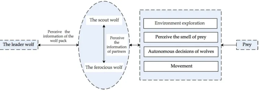
2.1. Wolf pack algorithm

Figure 1. Bionic graph of Wolf pack algorithm

：

The principle and steps of wolf pack algorithm are as follows

(1) Initialization of the wolf pack. Suppose that there are N artificial wolves in the D-dimensional space, and the location of the

i

th wolf is shown as follows:

1 2

( , ,..., ),1 ,1

i i i id

X  x x x  i N dD (1)

The initial position is generated by the Equation (2).

min ( max min)

id

x x rand x x (2)

Where rand is a uniformly distributed random number in [0,1], xmax and xmin are the upper and lower limits of the search space respectively.

(2) Generation of the leader wolf. The wolf at the optimal position of the target function value is chosen as the leader wolf. The leader wolf neither updates the position of the hunting process nor participate in hunting activities, but directly iterates. If Ylead Yi, then Ylead Yi，namely the scout

wolf becomes a leader wolf at this time. Conversely, if the scout wolf i migrates towards h directions until the maximum H is obtained or location cannot be further optimized, and the search stops at this moment. Among the h positions searched by the wolf i, the position of the jth point at the dth dimension is shown as follows：

ijd id a

y y randstep ₍₃₎

(3) Close to the prey. The location update of the wolf pack is promoted by the summoning behavior of the leader wolf. Driven by the summoning behavior, the new location is obtained by wolves based on the summons of the leader wolf. The updated position of wolf i at the d th dimension is shown as follows

：

( )

id id b id lid

z x rand step  x x (4)

Where stepa is the length of the wolf's stride in the search process, stepb is the length of stride

when the wolf moves to the target, xid is the current position of the wolf i at the dth dimension

and xlid is the position of the leader wolf at the dth dimension.

(4) Encirclement of the prey. After discovering the prey, the surrounding wolves will complete the reclamation of the target prey according to the signals issued by the leader wolf. Equations of the reclamation and the reclamation steps are as follows:

1 , ,

t

i m

t i

i m

X r θ

X

X rand ra r θ

  

 

  

 

min max

ln( / )

( )

max min max min

( ) ( )

ra ra t

ra t ra  x x e (6)

Where t is the number of iterations, ra is the length of the wolf's stride during the reclamation,

i

X is the position of the leader that issued the signals and t i

X is the position of the wolf i in the t th iteration.

(5) Update mechanism of wolves competition. Wolves will be eliminated without food in the process of reclamation hunting, instead the wolves that survived are the first to obtain food. Weak wolves that without food will be eliminated while an equal number of new wolves that are randomly generated will be added into the wolf pack.

2.2. Data inconsistency rate (DIR)

The feature selection of many historical cost data of substation projects takes aim at distinguishing the most relevant data features, which makes the input vector of the power projects cost forecasting model with a strong pertinence and reduces the redundancy of the input information in order to improve the accuracy of the cost forecasting of the substation projects. The inconsistency rate of data can accurately describe the discrete characteristics of the input features. Different feature characteristics can be obtained by different division modes and different division modes can obtain different frequency distributions. The discrimination ability of data categories can be distinguished by the inconsistency rate of calculation. The higher the inconsistency rate of data, the stronger the classification ability of feature vectors.

It’s necessary to know the specific calculation formula of the inconsistency rate for selecting the features by means of the inconsistency rate method. Therefore, it is assumed that the collected cost data of substation projects have g features, such as main transformer capacity, floor space, main transformer unit price, etc. which are respectively represented by the values of G1, 2,G , Gg.  is the feature set and L is a subset of the feature set. Next, set the standard class Mwith ccategories and Ndata instances. The feature value corresponding to the feature Fi is represented as zji. i is

the class value of M , then the data instance can be represented as [zj,i] , where

1 2 3

[ , , , , ]

j j j j jg

z  z z z  z . The calculation formula of the inconsistency rate is shown as follows:

1 1

max{ }

p c

kl kl

l k l

f f

N

  

 



 

 



 

₍₇₎

Where fkl is the number of data instances that centrally belongs to the feature subset of the xk

mode. xk is the data set with a total of Pfeature partition modes, where (k1, 2,,p and pN).

The feature selection on the basis of the inconsistency rate is shown as follows

：

(1) Initialize the optimal feature subset  to an empty set.

(2) Calculate the inconsistency rate of datasets G1, 2,G , Gg which belongs to the subset mode that consists of the subset  and each remaining feature.

(3) Calculate the inconsistency rate statistical table of the feature subsets and rank the inconsistent data from small to large.

(4) Select the feature subset L with the smallest number of features. If L  or L'/L is the

minimum of all adjacent inconsistency rate, then the optimal feature subset is L, where L' is the last feature subset adjacent to L.

between features in the selection process, which has a better presentation of all data information through the selected optimal features.

2.3. Improved least squares support vector machine (LSSVM) 2.3.1. Least squares support vector machine

Least squares support vector machine (LSSVM) is an extension of support vector machine (SVM). It constructs the optimal decision surface by projecting the input vector into the high-dimensional space non-linearly. Next, the inequalities of SVM are inverted into the equation sets by applying the risk minimization principle, which reduces complexity and speeds up the rate of calculation [28].

Suppose that





_i, _i





N₁ i

T x y



 is the given sample set, Nis the total number of samples. The regression model of the sample is shown as follows

：

 

T

 

y x w  x b ₍₈₎

Where 

 

 is the function that projects training samples into a high-dimensional space, w is the weighted vector and b is the offset parameter.

The optimization problem of LSSVM can be converted into the following function to solve [29]_. 2

1

1 1

min

2 2

N T

i i

w w γ 







₍₉₎

s t T

 

, 1, 2,3,

i i i

y w x  b  i N (10)

Where  is the penalty coefficient, which is used to balance the complexity and accuracy of the model. i is the estimation error. The above equations can be solved by converting them into the

Lagrangian function, which is detailed in 2.3.3.

2.3.2. Improved method of LSSVM

(1) Horizontal weighting of input vectors

The cost forecasting of substation projects is mostly a multi-input and single-output model. The values of the input vectors are horizontally distributed with the item serial number. And the influence of the actual value of the substation projects cost influencing factors on the final forecasting value can be reflected by means of the weighted processing. Therefore, the weighted processing of input vectors is shown as follows:





ˆi ki 1 n i, 1, 2, ,

x x    k  l (11)

Where xˆ_i is the weighted input vector, xki is the original input vector, k is the dimension

number of input vector and  is a constant.

(2) Longitudinal weighting of the training sample sets

The cost forecasting value is not only related to the elements in the input vectors, but also has a certain correlation with the sample groups, which means that the close sample has a greater influence on the forecasting value and the long-range sample has less influence on the forecasting value. Therefore, it’s necessary to reduce the influence of close samples on the forecasting model by assigning different degrees of subordination to the influencing factors of the current substation projects cost, but enhance the influence of the long-range samples on the forecasting model at the same time. The linear membership degree i is used to calculate the degree of the given

(1 ) / , 0 1

i i N i

     (12)

Where i is the degree of membership,  is a constant between [0,1] and i1, 2,,N.

Then the input sample set can be changed as follows

：



 









1, 1, 1 2, 2, 2 N, N, N



T  x y  x y   x y 

The determination of  affects the fitting performance of LSSVM directly [31]_{. The value of } can be obtained through the gray correlation coefficient and the calculation formulas are shown as follows：



0



(min) (max) ( ), ( ) (max) ki ki i ki ki

r x k x k 



  



   (13)

0( ) ( ) [0,1]

ki x k x ki 

    (14)











N k i

i

r

x

k

x

k

1

0

(

),

(

)



(15)

In this paper, where x0 Y Y, 



y y1, 2,,yN



since the forecasting model for ice transmission lines is usually a multi-input and single-output model.

2.3.3. Weighted least squares support vector machine

The improvement in the above section is applied to the LSSVM to get the weighted least squares support vector machine. The objective function is described as follows

：

2 1 1 2 2 N i i i 1

min w w γ 







T

ξ ₍₁₆₎

s t T

 

, 1, 2,3,

i i i

y w x  b  i N ₍₁₇₎

To solve the above problem, the Lagrangian function is established as follows:





2

 

1 1 1 1 , , , 2 2 N N T T

i i i i i i i i

i i

L w b α w w γ    w x b  y

 

 







_    _{ (18)}

Where i is the Lagrange multiplier. The variables of the function are deduced and the

derivation is equivalent to zero. The specific calculation is shown as follows:

 

1 1 0 0 0 0 0 0 N i i i N i i

i i i

T i i L w x w L b L γ L b y w α                     _{  }        _{  }     _{     }   (19)

Convert the equations to the following problem by eliminating w andi.

1 1

0

0 nT

n

b e

a y

e    I

     

 

     

   _{   }

  (20)

Where T

   

i i

x  x



  , en



1,1,...,1



T, α



α ,α ,1 2,αn



and

T

1 2 n

The Equation (21) is obtained as follows.

 

N i



i,



i 1

y x αK x x b



  (21)

Where K x x



_i,



is the kernel function. The wavelet kernel function





' 1 , N i i i i i x x

K x x

            is

selected to replace the Gaussian kernel function in the standard least squares support vector machine and the construction of the wavelet kernel function will be detailed in the next section. The wavelet kernel function is brought into y x( ) as follows

：

 

' 1 1 N N i i i i i i x x

y x  b



 

  

   

  (22)

2

( ) cos(1.75 ) exp( )

2

x

x x

    (23)

Finally, the regression model of the weighted least squares support vector machine is shown as

：

follows

 

2 1 1

1.75( ) ( )

cos[ ] exp[ ]

2

N N

i i i i

i i

i _i

x x x x

y x  b

             

  (24)

In this paper, the wavelet kernel function was used to replace the traditional radial basis kernel function, which is mainly based on the following considerations. a. The wavelet kernel function has the excellent specialty of describing the data information step by step, and the LSSVM that uses the wavelet kernel function as the kernel function can simulate any function with high precision. However, the traditional Gaussian function is relatively less effective. b. The wavelet kernel function is orthogonal or approximately orthogonal, while the traditional Gaussian kernel function is related or even redundant. c. The wavelet kernel function can analyze and process the multi-resolution of wavelet signals. Therefore, the nonlinear processing ability of the wavelet kernel function is better than the Gaussian kernel function, which can improve the generalization ability and robustness of the LSSVM regression model.

2.3.4. Construction of the wavelet kernel function

The kernel function of LSSVM is the inner product of two input spatial data points in a spatial feature and it has two obvious features. Firstly, k x x( , ) k x x( , ) is the symmetric function of inner product kernel variables. Secondly, the sum of the kernel functions on the same plane is a constant. In short, only when the kernel function satisfies the following two theorems can it become the kernel function of the least squares support vector machine [32]_.

(1) Mercer’s theorem ( , )

k x x is the continuous symmetric core that can be extended to the following form:



'



 

 

' 1

, i i i

i

k x x g x g x









(25)

Where i is a positive value. The following necessary and sufficient conditions need to be met

to ensure complete convergence of the above extensions.

' ' '

( , ) ( ) ( ) 0, , n

k x x g x g x dxdx  x xR

For all the functions of g( ) , the condition that 2

( ) 0

( )

n R

g

g  d

        



needs to be satisfied.

Where g x( )_i is the feature function, i is the eigenvalue and all of them are positive. Therefore,

it’s known that the kernel function ' ( , )

k x x  is a positive definite function.

(2) Smola and Scholkopf theorem

When the kernel function satisfies the Mercer's theorem, k x x( , ) can be used as the kernel equation of the least square support vector machine when it is proved to satisfy the following Equation (27).

/2

( )( ) (2 ) n _nexp( ( )) ( ) 0, n R

F x    J  x k x dx x R





    ₍₂₇₎

(3) Construction of the wavelet kernel function

When the wavelet kernel equation satisfies conditions that 2 ' ( )x L R( ) L R( )

   andˆ ( )x 0, and ˆ ( )x is the Fourier transform of ( )x . Then ( )x can be defined as follows[33]_.

1/ 2

,m( ) ( ) ( ),

x m

x x R



  





  ₍₂₈₎

Where  is the shrinkage coefficient, m is the horizontal float coefficient and 0,mR.

When f x( ) satisfies 2 ( ) ( )

f x L R , then f x( ) can be wavelet transformed as follows

：

1/ 2 *

( , ) ( ) (x m)

W  m  f x dx



 







₍₂₉₎

Where * ( )x

 is the complex conjugate function of ( )x . The wavelet transform function ( , )

W  m is reversible and can be used for reconstructing the original signals, then the following formula can be obtained.

1

, 2

( ) ( , ) _m( )d

f x C_ W  m_ x  dm



  

 



 

(30)

Where 2 ˆ | ( ) | | | w C dw w    





  and ˆ ( )w 



( ) exp(x Jwx dx) .

In the above equation, C is a constant. The wavelet decomposition theory is an infinite approximation to a set of functions based on linear combination of the wavelet functions. Suppose that ( )x is a one-dimensional function, then the multidimensional wavelet equation can be described according to the tensor theory as follows

：

1

( ) ( ), ,

l

lxd d

l x _i xi x R xi R

 



    (31)

In this way, the horizontal floating kernel function is constructed as follows

：

'

' 1

( , ) ( ) 0

l i i i i i x x

k x x  







  ，  ₍₃₂₎

 

/ 2

( ) (2 )l _lexp( ( )) ( ) 0

R

F k w   J wx k x dx





  ₍₃₃₎

In this paper, the Morlet wavelet mother function is chosen to prove the above equation, which ensures the generalization of the wavelet kernel function. Namely,

2 ( )x cos(1.75 ) exp(x x / 2)

   (34)

And k x x( , ) can be expressed as follows

：

2 2 ' ' ' 2 2 1 2 2 1

( , ) cos 1.75( ) exp

2 2

1.75

cos( ) exp( / 2 )

l _{i i i i}

i

l

i

i i

x x x x

k x x

X x         _   _   _{   }          _{   }      (35)

Where  can be obtained through the sample fitting. N

xR and , N i

x R

  . It can be seen from the above equation that the multi-dimensional wavelet function can be used as a kernel function of the multi-dimensional least squares support vector machine. And the mathematical proof process is shown as follows:

2 ' ' 2 1 2 ₂ 1 2 2 1

exp( ) ( )

exp( ) ( cos[1.75( )]exp( ) )

2

exp( 1.75 / ) exp( 1.75 / )

exp( ) ( ) exp( / 2 )

2

1 1.75

exp ( ) e

2 2 l l l R l i i i i R i l i i

i i i i

R i l i i i i

Jwx k x dx

x x

x x

Jwx dx

j x x

Jw x x dx

x j jw x              _                                   







2 2 2 2 1 1.75

xp ( )

2

2 (1.75 ) (1.75 )

exp( ) exp( )

2 2 2

l

i

i i i

R

l

i i

i

x j

jw x dx

w w                                   _    _  



(36)

Finally, the equation is obtained as follows

：

2 2

1

(1.75 ) (1.75 )

( )( ) ( )(exp( ) exp( ))

2 2 2

l

i i

i

w w

F x w   



 

     (37)

Where   0 _{, so} F  x w  0 _{. In addition, it can be concluded that the wavelet kernel} function can be used as the kernel function of least squares support vector machine.

2.4. DIR-ILSSVM Optimized by the WPA Algorithm

two sections. And finally, the substation projects cost of the test sample can be forecasted through retraining of the W-LSSVM regression model.

The specific steps for cost forecasting of substation projects are listed as follows

：

(1) Determine the initial candidate feature values. By combing the related references [34]-[36], in this paper, the candidate features of the influencing factors of substation projects cost are selected as follows, including the floor space, construction properties, substation voltage level, main transformer capacity, number of outlets on the high-voltage side, number of outlets on the low-voltage side, topography, duration, substation type, number of transformers, economic development level of the construction area, inflation rate, transformer single unit price, high-side circuit breaker unit price, high-side circuit breaker unit, low-voltage capacitor quantity, high-voltage fuse price, current transformer price, power capacitor price, reactor price, power bus price, arrester price, measuring instrument price, relay protection device price, signal system price, automatic device price, site leveling fee, foundation treatment fee, designer's skill level, number of accidents, deviation rate of project volume, construction progress level, days of rain and snow, etc. In the IR algorithm, the optimal feature subset needs to be initialized to an empty set, namely  {}.

(2) Initialize the parameters of WPA. Set the total number of wolf N = 50, the number of iterations t = 100, step a = 1.5, step b = 0.8, q = 6, h = 5.

(3) Calculate the inconsistency rate. After step (1) and step (2) are completed, the candidate features are gradually substituted into the IR feature selection model. Calculate the inconsistency rate of datasets G1, G2,, Gg which belongs to the subset mode that consists of the subset  and each

remaining feature. The feature Gi corresponding to the minimum inconsistency rate is selected as

the optimal feature.   



,Gi



is the updated optimal feature set.

(4) Determine the optimal feature subset and parameters of the optimal regression model. The current feature subset is substituted into the ILSSVM model to calculate the forecasting accuracy

 

r j in the learning process of the current cycle training sample, and the fitness function value

 

Fitness j of each cycle can be obtained. The optimal feature subset can be determined through the comparison of fitness function values between each generation. Determine whether each iteration reaches the stopping condition of the algorithm. If it is not satisfied, the new feature subset is reinitialized and the new cycle is entered until the optimal subset of the global optimal feature is obtained. It is important to note that the parameters of the ILSSVM model also need to be optimized and the initial value of  and  will be allocated randomly. The fitness function based on double factors of forecasting accuracy and feature selection quantity is constructed as follows:

1

( ) ( ( ) )

( )

Fitness j a r j b

Numfeature j

     ₍₃₈₎

Where Numfeature x

 

i is the optimal number of features selected for each iteration, a and b

are constants between [0,1]. The optimal feature quantity and the fitness function value are proportional to each other in each iteration, and the cost forecasting accuracy of substation projects is inversely proportional to the fitness function value.

Figure 2. The flow chart of WPA-DIR-ILSSVM

3. Case Study

3.1. Collection and processing of data

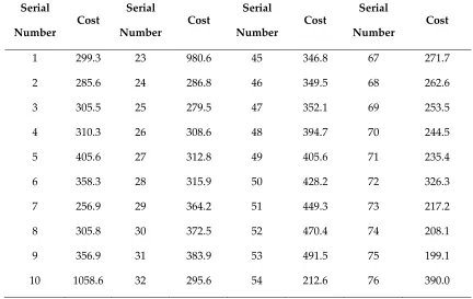
The relevant cost data of substation projects from 2015 to 2017 in different regions is collected in this paper, including 88 voltage level substation projects. The cost levels and the influencing factors of the first 66 substation projects are used as the training set, and the last 22 data sets are used as the test set. The collected original data of the substation projects cost is shown in Table 1.

Table 1. The collected original data of the substation projects cost (Unit: Yuan/kV·A)

Serial

Number

Cost

Serial

Number

Cost

Serial

Number

Cost

Serial

Number

Cost

1 299.3 23 980.6 45 346.8 67 271.7

2 285.6 24 286.8 46 349.5 68 262.6

3 305.5 25 279.5 47 352.1 69 253.5

4 310.3 26 308.6 48 394.7 70 244.5

5 405.6 27 312.8 49 405.6 71 235.4

6 358.3 28 315.9 50 428.2 72 326.3

7 256.9 29 364.2 51 449.3 73 217.2

8 305.8 30 372.5 52 470.4 74 208.1

9 356.9 31 383.9 53 491.5 75 199.1

11 501.2 33 270.2 55 353.7 77 280.9

12 208.6 34 260.8 56 254.8 78 285.1

13 356.2 35 239.3 57 375.9 79 289.4

14 401.5 36 381.7 58 397.0 80 293.7

15 378.6 37 406.9 59 418.1 81 297.9

16 369.5 38 315.6 60 335.3 82 402.2

17 301.6 39 285.5 61 326.2 83 306.4

18 325.8 40 333.7 62 317.1 84 310.7

19 337.1 41 336.3 63 308.0 85 274.9

20 368.9 42 309.0 64 298.9 86 319.2

21 370.2 43 341.6 65 289.9 87 283.4

22 450.1 44 244.2 66 280.8 88 369.5

The explanation of the processing of input indicators is shown as follows. The data of the construction properties of substation projects are mainly divided into three categories, in which the assignment of new substation is 1, the main transformer is 2 and t the interval project is 3. The data of the substation types are mainly divided into three categories, in which the assignment of the indoor type is 1, the half indoor type is 2 and the outdoor type is 3. The topography and landform are mainly divided into the following eight situations, in which the assignment of hillock is 1, slope is 2, plain is 3, flat ground is 4, paddy is 5, dry land is 6, mountain is 7 and muddy land is 8. The level of economic development in the construction area is based on the data of the local GNP and the technical level of the designers is based on the proportion of employees with bachelor degree or above in this project. The difference between the actual progress of the construction and the scheduled progress plan is selected to represent the construction progress level. And the data is normalized according to formula (39).

 

min

max min

1, 2,3,. ,

i i

x x

Y y i n

x x



  

  (39)

Where xi is the actual value, xmin and xmax are the minimum and maximum values of the

sample data, and yi is the normalized value.

3.2. Evaluation indicators of the forecasting results

Evaluation indicators of the cost forecasting results of substation projects adopted in this paper are shown as follows.

(1) Relative error (RE)

ˆ

100%

i i i

x x

RE x 

  ₍₄₀₎

(2) Root mean square error (RMSE)

2 1

ˆ 1

( )

n i i

i i

x x

RMSE

n  x







₍₄₁₎

1 1

ˆ

( ) / 100%

n

i i i i

MAPE x x x

n 





  ₍₄₂₎

(4) Average absolute error (AAE)

1 1

1 1

ˆ

( ) / ( )

n n

i i i

i i

AAE x x x

n  n 









(43)

In Equations (40) - (43) above, x is the actual value of the substation projects cost, xˆ is the forecasting value of the substation projects cost and n is the number of data groups. The smaller the value of above indicators, the higher the accuracy of cost forecasting.

3.3. Feature selection

The main content of this section is the selection of the optimal feature subset based on the DIR model, which helps determine the input indicators of the forecasting model. In this paper, Matlab R2014b is used to carry on the programming computation. The test platform environment is based on Intel Core i5-6300U, 4G memory and Windows 10 Pro edition system.

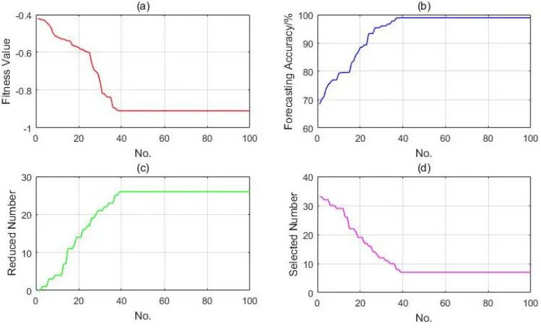
The iterative process diagram of the extraction of training sample features based on the WPA-DIR-ILSSVM model is shown as Figure 3. The accuracy curve shown in the figure describes the forecasting accuracy of ILSSVM for training samples in different iterations. The fitness curve describes the fitness function value calculated during each iteration. The selected number is the optimal number of features calculated by the DIR model in the process of convergence. And the reduced number of features refers to the number of features eliminated by the WPA algorithm during the convergence process.

Figure 3. The curve of convergence for feature selection

main transformer capacity, substation type, number of transformers, main transformer single unit price and floor space.

3.4. Cost forecasting of substation projects and results analysis

The input vectors are substituted into the ILSSVM model for training and testing after obtaining all the optimal features of the sample data. In this paper, the self-written program is used to run and calculate in Matlab software. It’s worth that the wavelet kernel function is chosen as the kernel function of the ILSSVM regression model in this paper. And the important parameters of the model are obtained through optimization based on WPA algorithm to ensure the accuracy of ILSSVM. The parameter settings of WPA have been given in section 2.4 and parameters of ILSSVM calculated by running the program are  43.0126 and  19.0382.

The unoptimized ILSSVM, LSSVM, SVM and BP neural networks (BPNN) are also selected to conduct the cost forecasting of substation projects, which helps prove the forecasting performance of the ice thickness forecasting model proposed in this paper. The topological structure of the BPNN model is 7-5-1, the transfer functions of the hidden layer and the output layer adopt the tansig function and purelin function, respectively. The maximum number of training is 200, the minimum error of the training target is 0.0001, the training rate is 0.1, and the initial weight and threshold are obtained by its own training. In the SVM model, the penalty parameter c is 10.276, the kernel function parameter  is 0.0013 and the loss function parameter  is 2.4375. In the LSSVM model,

c is 10.108,  is 0.0026 and  is 0.0018. And in the ILLSVM model, c is 16.263,  is 0.0012 and  is 0.0015.

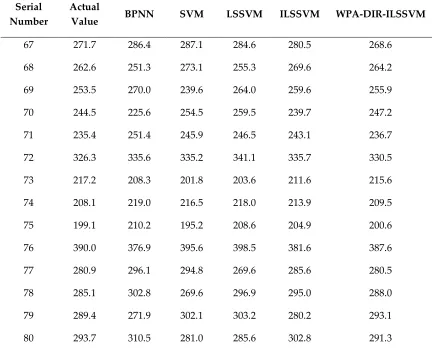
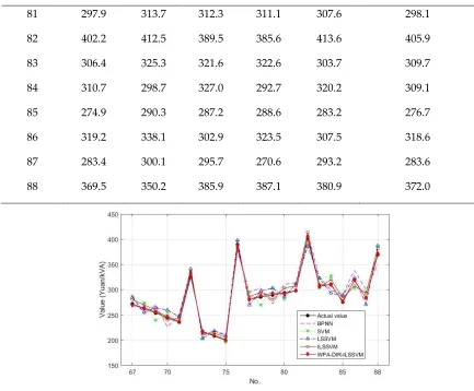
The forecasting results of BPNN, SVM, LSSVM, ILSSVM and the model constructed in this paper for cost forecasting of the test set are shown in Table 2.

Table 2. The forecasting values and actual values of the test set (Unit: Yuan/kV·A)

Serial Number

Actual

Value BPNN SVM LSSVM ILSSVM WPA-DIR-ILSSVM

67 271.7 286.4 287.1 284.6 280.5 268.6

68 262.6 251.3 273.1 255.3 269.6 264.2

69 253.5 270.0 239.6 264.0 259.6 255.9

70 244.5 225.6 254.5 259.5 239.7 247.2

71 235.4 251.4 245.9 246.5 243.1 236.7

72 326.3 335.6 335.2 341.1 335.7 330.5

73 217.2 208.3 201.8 203.6 211.6 215.6

74 208.1 219.0 216.5 218.0 213.9 209.5

75 199.1 210.2 195.2 208.6 204.9 200.6

76 390.0 376.9 395.6 398.5 381.6 387.6

77 280.9 296.1 294.8 269.6 285.6 280.5

78 285.1 302.8 269.6 296.9 295.0 288.0

79 289.4 271.9 302.1 303.2 280.2 293.1

81 297.9 313.7 312.3 311.1 307.6 298.1

82 402.2 412.5 389.5 385.6 413.6 405.9

83 306.4 325.3 321.6 322.6 303.7 309.7

84 310.7 298.7 327.0 292.7 320.2 309.1

85 274.9 290.3 287.2 288.6 283.2 276.7

86 319.2 338.1 302.9 323.5 307.5 318.6

87 283.4 300.1 295.7 270.6 293.2 283.6

88 369.5 350.2 385.9 387.1 380.9 372.0

Figure 4. Comparison of forecasting results of the test sets

Simultaneously, satisfactory forecasting results can be obtained by using the input vectors based on the DIR model. Additionally, ILSSVM presents more satisfactory performance than LSSVM, SVM and BPNN. This result indicates that the more accurate forecasting results can be achieved by means of the improvement of LSSVM.

Figure 5. RE of the forecasting results of the test set

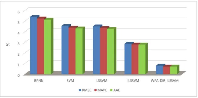
The RMSE, MAPE and AAE of BPNN, SVM, LSSVM, ILSSVM and WPA-DIR-ILSSVM are shown in Figure 6. From Figure 6, we can conclude that the RMSE, MAPE and AAE of the proposed model are 0.8025%, 0.7159% and 0.7157%, which are all the smallest among the above five models. In addition, the RMSE, MAPE and AAE of the ILSSVM model are 2.6858%, 2.7961% and 2.7956%, respectively. The RMSE, MAPE and AAE of the LSSVM model are 4.5163%, 4.3614% and 4.2778%, respectively. The RMSE, MAPE and AAE of the SVM model are 4.5558%, 4.3895% and 4.3203%. The RMSE, MAPE and AAE of the BPNN model are 5.5044%, 5.2589% and 5.1402%, respectively. The overall forecasting error of model the degree of error dispersion can be reflected through these indicators. Therefore, the overall forecasting effect of ILSSVM is better than that of LSSVM, SVM and BPNN, and the overall forecasting effect of LSSVM is better than that of SVM and BPNN, which indicates that the overall forecasting performance of LSSVM is significantly improved after the weighted improvement. The forecasting accuracy of WPA-DIR-ILSSVM is better than that of ILSSVM, which proves that the parameters  and  of ILSSVM selected by the WPA algorithm have a good optimization effect. And the DIR model ensures the integrity of the input information while reducing redundant data, in which the ideal forecasting results are achieved.

4. Conclusions

This paper presents a hybrid cost forecasting model that combines DIR with ILSSVM optimized by WPA. First, in order to forecast the substation projects cost, the DIR combined with the WPA is employed to select the input feature. Furthermore, the WPA is also adopted to optimize the parameters of the ILSSVM. Finally, after obtaining the optimized input subset and the best value of

 and  , the proposed model is utilized for the cost forecasting of substation projects. Several conclusions based on the studies can be obtained as follows: (a) by the utilization of DIR, the influence of unrelated noises can be reduced and the forecasting performance can be effectively improved. (b) the optimization algorithm WPA adds the model with strong global searching capability and the ILLSVM model optimized by WPA shows good performance. (c) based on the error valuation criteria. Compared with LSSVM, a better forecasting results can be achieved based on ILSSVM, which shows that the method of improving LSSVM by replacing the traditional radial basis kernel function with wavelet kernel function is effective. (d) Through the example verification of substation projects in different regions, different voltage grades and different scales, an ideal forecasting effect is obtained, which shows that the model proposed in this paper is more adaptable and stable. Hence the proposed cost forecasting method of WPA-DIR-ILSSVM is effective and feasible, and it may be an effective alternative for the cost forecasting in the electric-power industry.

Acknowledgments: 1. The paper is supported by Natural Science Foundation of China (Project No. 71471059). 2. The paper is supported by “the Fundamental Research Funds for the Central Universities (2018ZD14)”. 3. The paper is supported by the 111 project (B18021).

Author Contributions: In this research activity, all the authors were involved in the data collection and preprocessing phase, model constructing, empirical research, results analysis and discussion, and manuscript preparation. All authors have approved the submitted manuscript.

Conflicts of Interest: The authors declare no conflict of interest.

References

1. Leschert, D.; Iwasykiw, G.; Derworiz, R. Substation Grounding Transfer of Potential Case Studies. IEEE T. Ind. Appl.

2016, 52, 661-667. doi: 10.1109/TIA.2015.2463793.

2. González-Sotres, L.; Domingo, C. M.; Álvaro, S. M.; Miró, M. Large-Scale MV/LV Transformer Substation Planning Considering Network Costs and Flexible Area Decomposition. IEEE T. Power Deliver. 2013, 28, 2245-2253. doi: 10.1109/TPWRD.2013.2258944.

3. Hu, L.X. Research on Prediction of Architectural Engineering Cost based on the Time Series Method. J. Taiyuan Univ. Technol. 2012, 43, 706-709. doi: 10.3969/j.issn.1007-9432.2012.06.015.

4. Li, W. A Model of Building Project Cost Estimation Based on Multiple Structure Integral Linear Regression. Archit. Technol. 2015, 46, 846-849. doi: 10.3969/j.issn.1000-4726.2015.09.022.

5. Kim, B. C. Integrating Risk Assessment and Actual Performance for Probabilistic Project Cost Forecasting: A Second Moment Bayesian Model. IEEE T. Eng. Manage. 2015, 62, 158-170. doi: 10.1109/TEM.2015.2404935.

6. Hu, W. X. The Fundamental Research on Project Cost Forecast Model Based on GST. J. Cent. South. Univ. Forestry. Technol. 2011, 31, 146-150. doi: 10.3969/j.issn.1673-923X.2011.04.028.

7. Dong, S.; Zhang, Y.; He, Z.; Deng, N.; Yu, X.; Yao, S. Investigation of Support Vector Machine and Back Propagation Artificial Neural Network for performance prediction of the organic Rankine cycle system. Energy, 2018, 144, 851-864. doi: https://doi.org/10.1016/j.energy.2017.12.094.

Applying Artificial Neural Networks. Appl. Energ. 2016, 162, 218-230. doi: https://doi.org/10.1016/j.apenergy.2015.09.087.

9. Liu, J.; Ye, Q. Project Cost Prediction Model Based on BP and RBP Neural Networks in Xiamen City. J. Huaqiao Univ. Nat. Sci. 2013, 34, 576-580.

10. Ling, Y. P.; Yan, P. F.; Han, C. Z.; Yang, C. G. BP Neural Network Based Cost Prediction Model for Transmission Projects. Electric Power. 2012, 45, 95-99. doi: 10.3969/j.issn.1004-9649.2012.10.021.

11. Niu, D. X.; Wang, H. C.; Chen, H. Y.; Liang, Y. The General Regression Neural Network Based on the Fruit Fly Optimization Algorithm and the Data Inconsistency rate for Transmission Line Icing Prediction. Energies, 2017, 10, 2066. doi: 10.3390/en10122066.

12. Deo, R. C.; Wen, X.; Qi, F. A Wavelet-coupled Support Vector Machine Model for Forecasting Global Incident Solar Radiation Using Limited Meteorological Dataset. Appl. Energ. 2016, 168, 568-593. doi: 10.1016/j.apenergy.2016.01.130.

13. Wang, N. N.; Wang, F.; Yin, Y. T.; Li, H.; Hou, Y. Research on Cost Predicting of Power Transformation Projects Based on SVM. Construct. Econ. 2016, 37, 48-52. doi: 10.14181/j.cnki.1002-851x.201605048.

14. Song, Z. Y.; Niu, D. X.; Xiao, X. L.; Zhu, L. Substation Engineering Cost Forecasting Method Based on Modified Firefly Algorithm and Support Vector Machine. Electric Power. 2017, 50, 168-173. doi: 10.11930/j.issn.1004-9649.2017.03.168.06.

15. Yuan, X.; Tan, Q.; Lei, X.; Yuan, Y.; Wu, X. Wind Power Prediction Using Hybrid Autoregressive Fractionally Integrated Moving Average and Least Square Support Vector Machine. Energy, 2017, 129, 122-137. doi: https://doi.org/10.1016/j.energy.2017.04.094.

16. Huang, W. T.; Zhou, P.; Cheng, J. X. An Estimation Method of Engineering Cost Based on Adaboost and Variable Selection with LSSVM. J. Chongqing Jiaotong Univ. Nat. Sci. 2016, 35, 54-57. doi: 10.3969/j.issn.1674-0696.2016.03.12.

17. Liu, M. Prediction Model of Project Cost of Based on Chaotic Theory and Least Square Support Vector Machine. J. Inner Mongolia Normal Univ. Nat. Sci. 2015, 44, 333-338. doi: 10.3969/j.issn.1001-8735.2015.03.012.

18. Ruiz, G. R.; Bandera, C. F.; Temes, G. A.; Gutierrez, S. O. Genetic Algorithm for Building Envelope Calibration. Appl. Energ, 2016, 168, 691-705. doi: https://doi.org/10.1016/j.apenergy.2016.01.075.

19. Li, G.; Boukhatem, L.; Wu, J. Adaptive Quality-of-Service-Based Routing for Vehicular Ad Hoc Networks with Ant Colony Optimization. IEEE T. Veh. Technol, 2017, 66, 3249-3264. doi: 10.1109/TVT.2016.2586382.

20. Niu, D. X.; Liang, Y.; Wei, C. H. Wind Speed Forecasting Based on EMD and GRNN Optimized by FOA. Energies, 2017, 10, 2001. doi: 10.3390/en10122001.

21. Azaza, M.; Wallin, F. Multi Objective Particle Swarm Optimization of Hybrid Micro-Grid System: A Case Study in Sweden. Energy, 2017, 123, 108-118. doi: https://doi.org/10.1016/j.energy.2017.01.149.

22. Wu, S. H.; Zhang, F. M.; Wu, L. S. New Swarm Intelligence Algorithm—Wolf Pack Algorithm. J. Syst. Eng. Electron.

2013, 35, 2430-2438. doi: 10.3969/j.issn.1001-506X.2013.11.33.

24. Chen, T. M.; Ma, J. X.; Samuel, H. Huang.; Cai, J. M. Novel and Efficient Method on Feature Selection and Data Classification. J. Comput. Res. Development. 2012, 49, 735-745.

25. Ma, T. N.; Niu, D. X.; Huang, Y. L.; Du, Z. D. Short-Term Load Forecasting for Distributed Energy System Based on Spark Platform and Multi-Variable L2-Boosting Regression Model. Power Syst. Technol. 2016, 40, 1642-1649. doi: 10.13335/j.1000-3673.pst.2016.06.006.

26. Liu, J. P.; Li, C. L. The Short-Term Power Load Forecasting Based on Sperm Whale Algorithm and Wavelet Least Square Support Vector Machine with DWT-IR for Feature Selection. Sustainability, 2017, 9, 1188. doi: 10.3390/su9071188.

27. Xue, J. J.; Wang, Y.; Li, H.; Xiao, J. Y. A Smart Wolf Pack Algorithm and its Convergence Analysis. Contl. Decis. 2016, 31, 2131-2139. doi: 10.13195/j.kzyjc.2015.1202.

28. Lv, Y.; Hong, F.; Yang, T.; Fang, F.; Liu, J. A Dynamic Model for the Bed Temperature Prediction of Circulating Fluidized Bed Boilers Based on Least Squares Support Vector Machine with Real Operational Data. Energy. 2017, 124, 284-294. doi: https://doi.org/10.1016/j.energy.2017.02.031.

29. Barati-Harooni, A.; Najafi-Marghmaleki, A.; Arabloo, M.; Mohammadi, A. H. An Accurate CSA-LSSVM Model for Estimation of Densities of Ionic Liquids. J. Mol. Liq. 2016, 224, 954-964. doi: https://doi.org/10.1016/j.molliq.2016.10.027.

30. Malvoni, M.; Giorgi, M. G. D.; Congedo, P. M. Photovoltaic Forecast Based on Hybrid PCA–LSSVM Using Dimensionality Reducted Data. Neurocomputing. 2016, 211, 72-83. doi: https://doi.org/10.1016/j.molliq.2016.10.027.

31. Dong, R.; Xu, J.; Lin, B. ROI-based Study on Impact Factors of Distributed PV Projects by LSSVM-PSO. Energy. 2017, 124, 336-349. doi: https://doi.org/10.1016/j.energy.2017.02.056.

32. Wu, Q.; Peng, C. Wind Power Grid Connected Capacity Prediction Using LSSVM Optimized by the Bat Algorithm. Energies. 2016, 8, 14346-14360. doi: 10.3390/en81212428.

33. Kang, J.; Tang, L. W.; Zuo, X. Z.; Hao, L. I. Data Prediction and Fusion in A Sensor Network Based on Grey Wavelet Kernel Partial Least Squares. J. Shock.Vib. 2011, 30, 44-149.

34. Zhang, X. Analysis on the Influencing Factors of Project Cost in Substation Construction Stage. Low Carbon World.

2017, 33, 64-65.

35. Ni, W. Cost Control of Intelligent Substation. East China Electr. Power. 2014, 42, 601-607.