REAL AND REACTIVE POWER CONTROL OF HPFC WITH ADAPTIVE BACK STEPPING CONTROL

BACK STEPPING CONTROL

RAKESH BABU G

Electrical Department , Sri Vasavi Engineering College, Pedatadepalli, Tadepalligudem, Andhra pradesh, West Godavari Dist, India

K V BHARGAV

Electrical Department , Sri Vasavi Engineering College, Pedatadepalli, Tadepalligudem, Andhra pradesh,West Godavari Dist, India

CH RAMBABU

Electrical Department , Sri Vasavi Engineering College, Pedatadepalli, Tadepalligudem, Andhra pradesh, india

Abstract :This paper reports the investigation on the implementation of control technique based on Adaptive Back stepping Controller in a power system incorporating HYBRID POWER FLOW CONTROLLER(HPFC).The objective is to archive effective control of the real and reactive power flow in the line with minimum or zero dynamic interactions between them. Reference frame theory based mathematical models are used for analyzing the performance of the system in closed loop The effectiveness of newly proposed controller is observed through simulation studies using MATLAB/SIMULINK and the results are compared with the adaptive back stepping control of UPFC . The results obtained shows that the HPFC offers control characteristics similar to those of UPFC, and also shows that line can be loaded up to their thermal limits. And the new control technique contributes significantly towards the dynamic behavior of the HPFC under wide range of operating conditions. .

Keywords: Adaptive Back Stepping, Dynamic model, Flexible AC Transmission System, State space model, Unified Power Flow Controller, MATLAB/SIMULINK.

1.Introduction

The work presented in this project relates generally to the powers in an alternating current (AC) transmission system. In particular, it mainly to develop the newly proposed power flow controller [1] and uses the method [2] for controlling the flow of active and reactive power on an AC transmission line

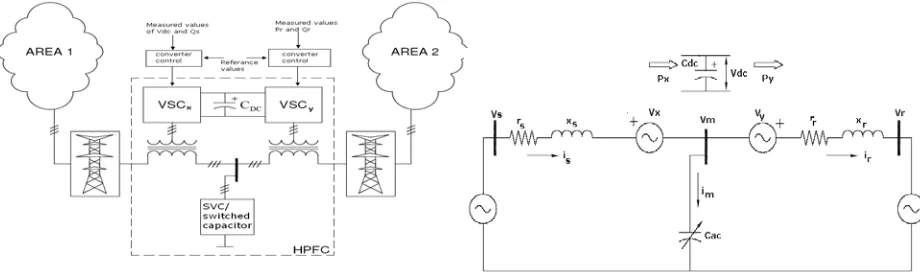
2. Basic principle of the HPFC

A block diagrammatic view of a typical HPFC application is shown in Figure. The HPFC is installed on a transmission line that connects two electrical areas.

Central to the HPFC’s topology is the shunt connected source of reactive power denoted by Cac in fig2.2 . This can be a switched capacitor bank, or a static VAR compensator. The key advantage of the HPFC over other known FACTS controllers is that it can be used to retrofit existing equipment. Therefore, its point of installation will often be dictated by the location of existing equipment, and in general it will be “within" the transmission line, i.e., at some distance from strong voltage buses.

A basic comparison of this topology with the topology of the UPFC[5,7] highlights the important features of the new circuit. In short, the UPFC’s shunt converter is substituted by an (often existing) SVC, while its series converter is split into two “half sized" ones, installed on each side of the shunt device. Consequently, considerable savings in the total required converter ratings can be achieved. Furthermore, the proposed topology gives rise to retrofit applications, as it permits the upgrade of the functionality of the SVC[5,6] (and, as will be shown, the switched capacitors). Since there is no need to decommission the SVC[5,6], the upgrading of its functionality can be done gradually. This means that the incremental addition of converters increase the functionality incrementally; an important advantage over the UPFC, as in its case the SVC[5,6] has first to be replaced resulting in the significant upfront cost.

3. Modeling of HPFC system

When switching functions are approximated by their fundamental frequency components neglecting harmonics, HPFC can be modeled by transforming the three phase voltages and currents to DQ variables using Park’s transformation which is given by

V_DQ =TV_abc --- (3.1) Where T is given by

( ) ( )

( ) ( )

2 1 2

1 2

1

120 sin 120 sin sin

120 cos 120 cos

cos

3 2 [T]

    

 

    

 

+ − − −

− − +

= θθ θθ θθ

3.1 modelling of AC shunt capacitor

The two series converters are represented by controllable voltage source Vx and Vy. Vm is the voltage at which shunt capacitor Cac is connected. Lr, Ls, rr, rs areinductanceand resistance of transmission line of both sides of HPFC.

Px is the real power exchange of the seriesconverter-1 with the DC link. Py is the real power exchange of the series converter-2 with DC link.

At any instant of time P_x =P_y ---- (3.2)

To develop the AC shunt capacitor model, apply KCL at bus-M, for three phases it is given by _ac V_{M abc} i_{m abc} i_s i_{r abc}

dt d

C [ ] =[ ] =[ − ] ---- (3.3)

Apply transformation method from three phase to DQ frame using Eq.(3.2) and taking the time derivative of these equations we get

_{Md Mq}

ac

Md i V

C V

dt d

ω + −

= 1 --- (3.4)

Mq Md

ac

Mq i V

C V

dt d

ω − −

= 1 --- (3.5)

Fig 2.1 HPFC detailed topological diagram

0 xb

V sb i . sb i . sb V

− _s − _s − −V_Mb= dt

d L

r

0 xc

V sc i . sc i . sc V

− s − s − −VMc=

dt d L

r --- (3.6)

Rewrite the above equations

s isabc rsisabc Vs Vx VM abc u abc

dt d

L [ ] + [ ] =[ − − ] =[1] --- (3.7) Where

[u1]abc =[Vs]abc −[Vx]abc −[VM]abc

The derivation for series converter-1 modeling for the eq (3.7) to convert into DQ frame follows same lines as described in previous section. Final the equations for series converter-1 is given by

i_sd ai_sd i_sq U_d1 dt

d

+ + −

= ω --- (3.8) i_sq wi_sd ai_sq U_q1 dt

d

+ − −

= --- (3.9) Where

s s

L r a=

s Md xd sd d

L V V V

U ₁ = − −

;

s

Mq xq sq q

L V V V

U ₁= − −

3.3 modeling of series converter-2

To develop the series converter-2 model apply KVL for the source end and converter-2 in fig.2.2. For three phases it is given by

₀

ya V ra i . ra i . Ma V

− r − r + −Vra =

dt d L

r

₀

yb V rb i . rb i . Mb V

− r − r + −Vrb =

dt d L

r

V_Mc− _r.i_rc− ._r i_rc +V_yc−V_rc =0

dt d L

r --- (3.10)

Rewrite the above equations

r irabc rrirabc VM Vy Vrabc u abc

dt d

L [ ] + [ ] =[ + − ] =[2] --- (3.11)

Where

[u2]abc =[VM]abc+[Vy]abc −[Vr]abc

The derivation for series converter-2 modeling for the eq (3.11) to convert into DQ frame follows same lines as described in above sections. Final the equations for series converter-2 is given by

i_rd bi_sd i_rq U_d2 dt

d

+ + −

= ω --- (3.12) i_rq wi_rd bi_rq U_q2

dt d

+ − −

= --- (3.13) Where

r rq yq Mq q r

rd yd Md d

r r

L V V V U L

V V V U

L r b

− + = −

+ = =

2

2 ,

3.4 modeling of dc link capacitor

The simplified equivalent circuit of the DC link between two converters is shown in below fig.3.1. To maintain fixed charge on Cdc in steady state condition, the converters represented by voltage source Vx and Vy have to operate under the constraint of power balance.

The differential equation describing the dynamics of Vdc ) ( 1 y x dc dc

dc P P

V dt dV

C = −

) rq .i yq V rd .i yd V .i V .i V ( 2 3 sq xq sd

xd + − −

= dc dc dc V C V dt d , )] ) rq .i yq V rd .i yd (V 2 3 ( -)) .i V .i (V 2 3 [( 1 sq xq sd

xd + +

= dc dc dc V V dt d

C --- (3.15)

4. ADAPTIVE CONTROL DESIGN[4] FOR HPFC SYSTEM BASED ON BACKSTEPPING CONTROL TECHNIQUE[4]

4.1 Control design for the series converter-1

The set of equations which represents series converter-1 in DQ axis are, rewrite the eqns (3.8) and (3.9) 1

d sq sd

sd ai i U

i dt d + + − = ω 1 q sq sd

sq wi ai U

i dt d + − −

= --- (4.1)

Let define state variable matrix

    =     = 2 1 x x i i X sq sd

Input matrix is

    − − − − =     s Mq xq sq s Md xd sd q d L V V V L V V V U U / ) ( / ) ( 1 1

The mathematical model for shunt converter is rewritten as 1 2 1 2 1 2 1 1 q d U ax wx x U wx ax x + − − =− + + = 

 _{--- (4.2)}

STEP-I: Define 2 2 2 1 1 1 x x Z x x Z ref ref − = − =

The time derivative of

Z

₁ and

Z

₂ is given by

1 1 2 1 2 2 2 2 1 1 2 1 1 1 1 1 q q ref ref d d ref ref U ax wx x x x Z U wx ax x x x Z

θ

θ

− − + + = − = − = + − − − =        

Where θd1andθq1 are uncertainties.

Choose a positive definite Lyapunov function

2 1 1 2 2 1 1 1 2 2 2 1

0 (ˆ )

2 1 ) ˆ ( 2 1 ] [ 2 1 q q d d p n m m Z Z L

V = + + θ −θ + θ −θ --- (4.3)

Where θˆd1,θˆq1 are estimates of θd1andθq1 m1 m2 are gains.

Time derivative of Vno is given by 1 1 1

2 1 1 1 1 2 2 1 1

0 (ˆ )ˆ

1 ˆ ) ˆ ( 1 q q q d d d p p n m m Z Z L Z Z L

V =  +  + θ −θ θ + θ −θ θ

) 2 1 ˆ 2 )( 1 1 ˆ ( ) 1 1 ˆ 1 )( 1 ˆ ( ) 1 1 2 ( 2 ) 1 2 1 1 ( 1 ) ˆ ( ˆ ) ˆ ( _ ) ˆ ( ˆ ) ˆ ( ) ( ) ( 2 2 1 2 1 2 1 2 1 1 1 1 1 1 1 1 1 1 2 1 2 2 1 2 1 1 1 m q Z p L q q m d Z p L d d q U ax wx ref x Z p L d U wx ax ref x Z p L m Z L m Z L m Z L m Z L U ax wx x Z L U wx ax x Z

L d _{q p} q _{q p} q

p d d p d q ref p d ref p θ θ θ θ θ θ θ θ θ θ θ θ θ θ + − + + − + − + + + − − + = + + + + + + − − + + + − − + =        

From Lyapunov theorem -I

Then V_v0=−[K_n1L_pZ₁2+K_n2L_pZ₂2]

is negative definite for K_n1>0and K_n2 >0 4.2 Control design for the series converter-2

The set of equations which represents series converter-2 in DQ axis are, rewrite eq. (3.12) & (3.13) 2

d rq sd

rd bi i U

i dt d + + − = ω 2 q rq rd

rq wi bi U

i dt d + − −

= -- (4.5)

Let define state variable matrix

    =     = 4 3 x x i i X rq rd Input matrix is

    − + − + =     r rq yq Mq r rd yd Md q d L V V V L V V V U U / ) ( / ) ( 2 2

The mathematical model for series converter is rewritten as 2 4 3 4 2 4 3 3 q d U ax wx x U wx bx x + − − =− + + = 

 _{--- (4.6)}

STEP-I: Define 4 4 4 3 3 3 x x Z x x Z ref ref − = − =

The time derivative of

Z

₃ and Z₄ is given by

2 2 4 3 4 4 4 4 2 2 4 3 3 3 3 3 q q ref ref d d ref ref U ax wx x x x Z U wx ax x x x Z θ θ − − + + = − = − = + − − − =        

where

θ

_d2

and

θ

_q2 are uncertainties. Choose a positive definite Lyapunov function

2 2 2 4 2 2 2 3 2 4 2 3

0 (ˆ )

2 1 ) ˆ ( 2 1 ] [ 2 1 q q d d m m m Z Z L

V = + + θ −θ + θ −θ --- (4.7)

where

θ

ˆd₁,

θ

ˆq₁ are estimates of

θ

d1and

θ

q1; m1 m2 are gains. Time derivative of Vmo is given by

) ˆ )( ˆ ( ) ˆ )( ˆ ( ) ( ) ( ˆ ) ˆ ( 1 ˆ ) ˆ ( 1 4 2 4 2 2 3 2 3 2 2 2 4 3 4 4 2 4 3 3 3 2 2 2 4 2 2 2 3 4 4 3 3 0 m Z L m Z L U bx wx x Z L U wx bx x Z L m m Z Z L Z Z L V q q q d d d q ref d ref q q q d d d m θ θ θ θ θ θ θ θ θ θ θ θ + − + + − + − + + + − − + = − + − + + =       

From Lyapunov theorem -I

For exiting equilibrium state at origin, is asymptotically stable then the Lyapunov function should be positive definite and its first derivative should be negative definite.To make negative definite

V



_m0 negative definite choose 4 4 2 3 3 2 ˆ ˆ Z m L Z m L q d − = − = θ θ   4 4 2 4 3 4 2 3 3 2 4 3 3 2 ˆ ˆ Z K bx wx x U Z K wx bx x U n q ef q n d ref d + − + + = + − − + = θθ 

Then Vm0 =−[Kn3L Z32+Kn4LZ42]

is negative definite for K_n1>0and K_n2 >0

Fig 3.1 Block diagram representation for adaptive back stepping control of HPFC

5. SIMULATION RESULTS AND DISCUSSIONS

The per-phase equivalent circuit of a simple two machine system is shown in Fig.2.2. Vs,

V

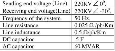
r represent balanced three-phase sinusoidal voltages where the receiving end voltage lags the sending end voltage by an angle of 300. The line parameters and other details of the system of Fig. 2.2 are given in TABLE 5.1. Table 5.1Details of parameters

Sending end voltage (Line) 220KV

∠

00. Receiving end voltage(Line) 220KV

∠

-300. Frequency of the system 50 Hz.

Line resistance 0.025 Ω /ph/Km Line inductance 0.5 Ω/ph/Km

DC capacitor .5 F

AC capacitor 60 MVAR

For the basic system with selected parameters the power flows at the receiving end, without HPFC are obtained as

Pr = 236.9 MW (active power) Qr = -76.29 MVAR (reactive power)

At t<1.2s, the system operates in normal condition. At t=1.2s, various input commands are given in separate cases of investigation. Five cases are considered for simulations:

1 Increase of Active power reference from 236.9 MW to 435.3 MW. 2 Decrease of Active power reference from 236.9 MW to 53.35 MW.

3 Increase of Reactive power reference from -76.29 MVAR to -231.6 MVAR. 4 Decrease of Reactive power reference from -76.29 MVAR to 148.5 MVAR 5 Sequential Control of Real and Reactive Power.

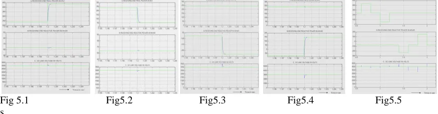
Simulation results for all the cases are illustrated in figures below Case 1: Active Power Control --Increase of real power

At time t=1.2s, when active power flow reference alone is changed from 236.9 M W to 435.3 M W and reactive power reference is unchanged. The active power flow changes from 236.9 M W to 435.3 M W, obtained within a negligible time less than 0.0004s as in fig, whereas the reactive power after a small transient rise in reactive power, at about 0.0004s settles at -76.29 MVAR as in fig, and the DC link voltage is increased by 200 volt at 1.2s, which is settled completely at 3000V reference as in fig5.1.

Case 2: Active Power Control ---Decrease of active power

At time t=1.2s, when active power flow reference alone is changed from 236.9 M W to 53.35 M W and reactive power reference is unchanged. The active power flow changes from 236.9 M W to 435.3 M W,

Ser

ies conver

ter

s 1 &

2, Dc

link

ca

p

acitor

and AC s

231.6 MVAR, obtained within a negligible time about 0.0005s as in fig, whereas the active power after a small transient rise in power, at about 0.0005s settles at 236.9 MW as in fig, and the DC link voltage is decreased by 120 volt at 1.2s, which is settled completely at 3000V reference as in fig5.3

Case 4: Reactive Power Control ---Decrease of reactive power

At time t=1.2s, when reactive power flow reference alone is changed from -76.29 MVAR to 148.5 MVAR and active power reference is unchanged. The reactive power flow changes from -76.29 MVAR to 148.5 MVAR, obtained within a negligible time about 0.00045s as in fig, whereas the active power after a small transient decrease in power, at about 0.0005s settles at 236.9 M W as in fig., and the DC link voltage is decreased by 145 volt at 1.2s, which is settled completed at 3000V reference as in fig5.4

Case 5: Sequential increase and decrease of Real and Reactive power control:

In this case, the time period 0- 2 sec is divided into 5 sections. At the beginning of each section, either real or reactive power commands are changed. First at t=0, power command given to HPFC are Prref = 236.9 MW and Qrref=-76.29 MVAR. In the second section i.e. at t=0.6s, power command given to HPFC are Prref = 435.3 MW and Qrref= -76.29 M. In the third section i.e. at t=0.8s, power command given to HPFC are Prref = 236.9 MW and Qrref=-76.29 M. In the fourth section i.e. at t=1s, power command given to HPFC are Prref = 53.35 MW and Qrref =-76.29 M VAR. In the fifth section i.e. at t=1.2s, power command given to HPFC are Prref = 236.9 MW and Qrref =-76.29 M VAR. In the sixth section i.e. at t=1.4s, power command given to HPFC are Prref = 236.9 MW and Qrref=-231.6 M VAR. In the seventh section i.e. at t=1.6s, power command given to HPFC are Prref = 236.9 MW and Qrref=-76.29 M VAR. In the eighth section i.e. at t=1.8s, power command given to HPFC are Prref = 236.9 MW and Qrref= 148.5 M VAR and finally the ninth section i.e. at t=2s, power command to HPFC are Prref = 236.9 MW and Qrref=-76.29 MVAR. In all the sections it can be seen that real and reactive power settles exactly at the reference value. Simulation results for this case are shown in the Fig. the DC link voltage also settles at reference 3000V as in fig5.5

Fig 5.1 Fig5.2 Fig5.3 Fig5.4 Fig5.5 s

6. CONCLUSIONS

A complete structure of the controller based on Backstepping for dynamic control of HPFC developed. The controller’s performance has been verified with sudden change in receiving end powers, using MATLAB/SIMULINK mathematical models. The simulation results obtained are discussed in each case. With this, it can be concluded that during system transients, the HPFC is capable to temporarily leave the manifold of equal power exchange and return to it in steady state. The time required to reach the reference value are also negligible.

From the various studies, the HPFC functionality is similar to UPFC. The key benefit of the new topology is that it fully utilizes existing equipment and therefore the required ratings of the converters are substantially lower than the rating of the comparable UPFC [2, 3].

References

[1] Jovan Z.Bebic, Peter W.Lehn and M.R. Irravani, “The Hybrid Power Flow Controller; A New Concept For The Flexible AC Transmission”, IEEE 2006

[2] Independent Control of Real and Reactive Power Flows using UPFC based on Adaptive Back Stepping G. Saravana Ilango, C. Nagamani and D. Aravindan National Institute of Technology/EEE, Tiruchirappalli, India IEE transactions 2008

[3] Dynamic Decoupled Compensator for UPFC Control C. M. Yam, and M. H. Haque, 2002 IEEE.

[4] P.V.Kokotovic, “The Joy of feedback: nonlinear and adaptive’, IEEE Trans. Control System,Technol.12(1992) 7-17.

[6] C.Schader, H.mehta, “Vector analysis and control of advanced static VAR compensator”, IEE proceedings-C, vol.140,No.4,July 1993. [7] Dr. L. Gyugyi, “Unified power flow control concept for flexible AC transmission systems”, IEE