The determinants of urban household poverty in Malaysia

The Determinants of Urban Household Poverty in

Malaysia

Mok, T.Y.1, C. Gan1 and A. Sanyal1

1 _{Commerce Division, Lincoln University, Canterbury, New Zealand}

Email: mokt2@lincoln.ac.nz

Keywords: Urban poverty, logistic regression, sensitivity analysis

EXTENDED ABSTRACT

Since independence in 1950s Malaysia has been recognised as one of the more successful countries in fighting poverty: head count ratio came down to 5.7 percent by 2004. However the recent process of rapid urbanization has led to an increase of urban poverty aggravated further by the 1997 Asian financial crisis. It is important to understand the nature and scale of urbanization, the various driving forces that affect it and the determinants of urban poverty as linked to this process. Our paper identifies the determinants of urban poverty in Malaysia using a logistic regression. Multiple regression model which used to be the main tool of analysis in this kind of studies has been criticised for a number of drawbacks and binary probit or logit models have been proposed as alternative and widely used (see Gaiha, 1988; Lanjouw & Stern, 1991; Grootaert, 1997). Our paper follows this methodology.

Previous studies have used income to identify poor households. We have two problems with this procedure. First, the official poverty line in Malaysia is an consumption expenditure. Secondly data on household incomes are known to be less reliable than consumption data obtained from household expenditure surveys. We therefore compare a person’s consumption expenditure with the poverty line to determine its poverty status. This agrees with the idea that poverty is the inability to attain a critical minimum amount of consumption. We study the effect of human capital, region of residence and other household characteristics on urban poverty using this benchmark

A sample of 2,403 urban households from the 2004-05 Household Expenditure Survey (HES) has been used in this research. We first estimate the probability of households with specified characteristics to fall below Malaysia’s official poverty line. Results show that human capital

significantly reduces the chance of being poor while migrant workers are more prone to poverty. Household size, race and regions are also important determinants of poverty outcome in urban Malaysia. Then we analyse the sensitivity of the probability estimates to shift of the poverty line over a reasonable range. Effects of education, number of children, number of male adults, number of elderly, foreign migrant-headed household, Chinese household and households living in Region 1 on poverty are robust over the shifts. The findings have important policy implications for Malaysian government which has pledged to reduce overall poverty rate to 2.8 percent and eradicate hardcore poverty by 2010 under the Ninth Malaysian Plan.

1. INTRODUCTION

Malaysia had successfully reduced the incidence of poverty from 52.4 to 5.1 percent between 1970 and 2002. Total number of poor households fell from 1.6 million to 267,000 over this period (Ahmad, 2005). This trend was however getting disturbed, unnoticed at the time, by the country’s fast economic growth and rapid urbanization of the 1990s. The urban population swelled from 30 percent in 1960 to 40 percent in 1980 and to 60 percent in 2000 (World Bank, 2007). According to the United Nations Population Division, 78 percent of the country’s population will be urbanised in 2030. The acceleration of urbanization has been accompanied by increase of urban poverty together with crowding, uneven distribution of development benefits and change in the ecology of urban environments.

When the economic boom (late 1980s and the 1990s) ended with the Asian financial crisis (1997), the country found itself in economic hardship, high unemployment and growing income inequality. The crisis of 1997 adversely affected the urban poor and migrant workers through job loss, rise of food prices and general inflation. Overall incidence of poverty increased from 6.8 percent in 1997 to 8.1 percent in 1999. The number of poor households increased to 393,900 in 1999 (Nair, 2000). Unemployment rate increased from 2.6 to 3.9 percent between 1996 and 1998 as the number of retrenched workers more than doubled from 8,000 to 19,000 between 1996 and 1997. Most retrenched workers were from manufacturing and construction sectors, thus affecting female workers, the urban poor and foreign workers who make up large parts of the labour force in these sectors (Nair, 2000). In the country as a whole, income share of the bottom 40 percent fell from 14.5 to 13.5 percent while that of the top 20 percent increased from 50 to 51.2 percent between 1990 and 2004 (Economic Planning Unit, 2006). The government now faced the renewed challenge of reducing wealth and income inequality among and between ethnicities and regions and particularly in urban areas.

Given the changing dimensions and emerging new forms of poverty there is a need to re-examine urban poverty in Malaysia. This paper identifies the determinants of urban poverty in Peninsular Malaysia, Sabah and Sarawak.

The paper is organized as follows: Section 2 describes the data, variables and methodology. Section 3 discusses the empirical results and conclusions and their implications are discussed in section 4.

2. METHODOLOGY

2.1. Data

Data for this research is obtained from Household Expenditure Survey (HES) conducted by the Department of Statistics, Government of Malaysia. The most recent HES of 2005 is our main source. This survey covers urban and rural areas of Peninsular Malaysia, Sabah and Sarawak except the interior areas of Sabah, Sarawak and the indigenous settlements (the Orang Asli). HES records a comprehensive expenditure of households including durables, semi durables and services for 12 months. In addition, it records a range of household characteristics. From this survey, a sample of 2,403 households in urban areas for the whole of Malaysia has been used for our research.

2.2. Model Specification

We use a binomial logistic regression model given that the dependent variable is dichotomous: 0 when a household is above and 1 when below the poverty line. Predictor variables are a set of socioeconomic and demographic status indicators and human capital and dwelling endowment of the household. They contain both dichotomous and continuous variables. Let Pj denote the probability that the j-th household is below the poverty line. We assume that Pj is a Bernouli variable and its distribution depends on the vector of predictors X, so that

( ) 1

X

j X

e P X

e

α β

α β +

+ =

+ ₍₁₎

where β is a row vector and α a scalar. The logit function to be estimated is then written as

ln 1

j

i ij i j P

X P = +α β

−

∑

The logit variable ln{Pj/(1-Pj)}is the natural log of

does not require assumptions of normality or homoskedasticity of errors in predictor variables.

Demographic variables:

Age_hh (-) = age of household head (in years) Sqage (+) = age squared,

Sex (+) = 1 if household is female, 0

otherwise, Child15 (+) = number of children under 15

years old,

Madults (+) = number of male adults in household,

Fadults (+) = number of female adults in household,

Elderly (+) = number of elderly (

≥

otherwise,

Migrant (+) = 1 if household is a foreign migrant, 0 otherwise, Race 1 = 1 if household is Malay, 0

otherwise,

Race 2 = 1 if household is Chinese, 0 otherwise,

Race 3 = 1 if household is Indian, 0 otherwise,

Socioeconomic status:

Industry_hh (+) = 1 if industry is secondary sector, 0 otherwise,

Status (+) = 1 if household doesn’t own its living quarter; 0 otherwise, Human capital variable:

Hi_fed (-) = highest formal education obtained by household head (in years),

Region variable:

Region 1 = 1 if Western region (incl. Kelantan, Terengganu, Pahang), 0 otherwise,

Region 2 = 1 if Northern region (incl. Kedah, Penang, Perak, Perlis), 0 otherwise,

Region 3 = 1 of Eastern region (incl. Sabah, Sarawak, Labuan), 0 otherwise,

α = intercept term

We have first estimated the model using the expenditure cut off point corresponding to Malaysia’s official poverty line: per capita consumption expenditure of RM 155. This forms a benchmark. Then we have allowed some variation of the line and reworked the logistic estimates to study the robustness of qualitative conclusions. Due to the lack of definiteness in any poverty line specification, sensitivity analysis is important to ensure which predictors are robust over reasonable

shift of the line (Grootaert, 1997; Serumaga-Zake & Naude, 2002). Section 3 reports comparison over a range of poverty lines.

A priori hypotheses are indicated by (+) or (-) in the above specification. The age variable expects to account for the effect of work experience while the squared variable expects to capture the opposite effect of declining ability with age. Human capital is measured by education level. Marital, Madults and Fadults do not provide unambiguous a priori expectation because a married head or a larger family may face the prospect of extra burden as well as extra income and possible economy of scale. Race variables represent the three main races of Malaysia.

Organisations in the primary sector are classified as large, diversified, capital intensive and offer higher pay and opportunities. In comparison, firms in secondary are smaller, labour-intensive and offer lower pay and opportunity for career enhancement (Thompson & McDowell, 1994). It is believed that ceteris paribus a person employed in the secondary sector is more likely to be in poverty. Ownership status of dwelling is included because owning an asset would lower the risk of a household falling into poverty. It could function as shelter, as collateral for borrowing and be sold during bad times and helps income smoothing over time (Grootaert, 1997).

Dummy variables have been used for regions, sex, marital status of household head, foreign migrant, races, and industry.

3. EMPIRICAL FINDINGS

Table 1. Mean and Standard Deviation of predictors by expenditure quartiles. Note: Mean is the main entry and standard

deviation is in parenthesis.

Variables 25th

percentile or less

50th

percentile or less

75th

percentile or less

Above 75th

percentile Age_hh 46.15

(11.78)

45.35 (12.59)

46.11 (12.84)

45.28 (12.97)

Sex 0.10

(0.299) 0.10 (0.29)

0.14 (0.35)

0.12 (0.32)

Marital 0.10

(0.30)

0.11 (0.32)

0.12 (0.33)

0.18 (0.38) Hi_fed 5.10

(2.815) 6.41 (2.79)

6.82 (3.03)

8.09 (3.00)

Industry 0.33

(0.471) 0.31 (0.46)

0.31 (0.46)

0.36 (0.48)

Status 0.44

(0.497) 0.36 (0.48)

0.32 (0.47)

0.32 (0.47)

(1.88) (1.60) (1.29) (1.29) Madult 1.49 (1.07) 1.48 (1.31) 1.35 (0.97) 1.18 (0.86) Fadult 1.56 (0.81) 1.50 (1.03) 1.43 (0.99) 1.28 (0.84)

Elderly 0.51

(0.77) 0.43 (0.70) 0.48 (0.78) 0.42 (0.75) Migrant 0.06 (0.23) 0.01 (0.10) 0.02 (0.14) 0.01 (0.08) Malays 0.58 (0.49) 0.58 (0.49) 0.5 (0.5) 0.43 (0.49) Chinese 0.15 (0.36) 0.22 (0.41) 0.34 (0.47) 0.43 (0.49) Indians 0.08 (0.27) 0.12 (0.33) 0.08 (0.27) 0.10 (0.29)

Region 1 0.15

(0.36) 0.11 (0.32) 0.08 (0.27) 0.04 (0.19)

Region 2 0.19

(0.39) 0.23 (0.42) 0.22 (0.42) 0.15 (0.36)

Region 3 0.25

(0.43) 0.14 (0.34) 0.13 (0.33) 0.12 (0.33)

Table 1 presents the descriptive statistics of predictors by expenditure quartiles. It shows that means of the variables hi_fed, marital and Chinese increase over the quartiles, while status, child15, madult, fadult, elderly, migrant, Malays, region 1, 2 and 3 fall with increasing per capita expenditure. For example, fewer higher educated households are in poverty than uneducated households. These distributions provide us with a priori expectations. In addition, the decreasing number of children, male adult, female adult and elderly households with increasing per capita expenditure shows the emergence of the nuclear family in higher income households in urban areas of Malaysia.

3.1. Determinants of Urban Poverty

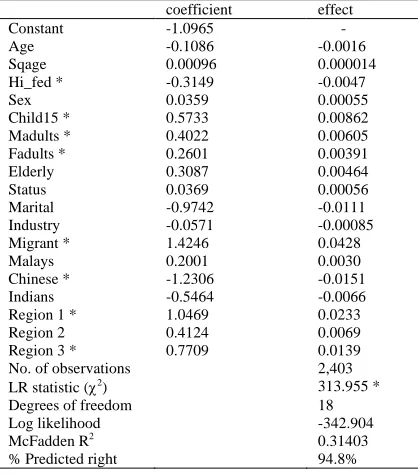
The estimates of the logistic regression are shown in Table 2. In general, the logit model fitted the data quite well. The chi-square test strongly rejects the hypothesis of no explanatory power and the model correctly predicted 94.8 percent of the observations. Furthermore, Hi_fed, Child15, Madults, Fadults, Migrant, Region 1, and Region 3 are statistically significant and the signs on the parameter estimates support expectations. The variable Chinese supports the observations of Table 1.

Table 2. Logistic model (Poverty Line RM155). Note: Marginal effect is evaluated at the mean value of predictor variables. For dummy variable,

marginal effect is P|1-P|0.

* denote statistically significant at 5% significance level.

Variables Estimated Marginal

coefficient effect

Constant -1.0965 -

Age -0.1086 -0.0016

Sqage 0.00096 0.000014

Hi_fed * -0.3149 -0.0047

Sex 0.0359 0.00055

Child15 * 0.5733 0.00862

Madults * 0.4022 0.00605

Fadults * 0.2601 0.00391

Elderly 0.3087 0.00464

Status 0.0369 0.00056

Marital -0.9742 -0.0111

Industry -0.0571 -0.00085

Migrant * 1.4246 0.0428

Malays 0.2001 0.0030

Chinese * -1.2306 -0.0151

Indians -0.5464 -0.0066

Region 1 * 1.0469 0.0233

Region 2 0.4124 0.0069

Region 3 * 0.7709 0.0139

No. of observations 2,403

LR statistic (χ2_{) 313.955 *}

Degrees of freedom 18

Log likelihood -342.904

McFadden R2 _0.31403

% Predicted right 94.8%

The results show education is an important determinant, which supports the findings of most previous researches (Thompson & McDowell, 1994; Rodriguez & Smith, 1994; Grootaert, 1995; Zake & Naude, 2002). Additional insight can be obtained through analysis of the marginal effects calculated as the partial derivatives of the non-linear probability function, evaluated at each variable’s sample mean (Greene, 1990). For example, an increase of a year of formal education after the mean number of years of the sample reduces the probability of a household falling into poverty by 0.0047. The results also show that a higher proportion of children under 15 years of age, female and male adults in the household increase the probability of a household falling into poverty. Number of children is generally found to be associated with poverty in most studies cutting across the developing world. Secondly, both genders (almost) equally increase the probability of being poor thus indicating low level of gender discrimination in urban Malaysia. This could be the result of local governments providing childcare assistance to encourage women to work and the work of non-government organizations (NGOs) towards female-empowerment.

foreign workers in Malaysia earn less than their Malaysian counterparts. Thus, the existence of market segmentation and discrimination in the job market has increased the risk of foreign workers falling into poverty.

Notably, the variable Chinese has a negative and significant coefficient. This suggests relatively higher employment and business opportunities for the Chinese compared to other races. Lim (1994) found that the incidences of poverty in three new Chinese villages were lower compared to the average for Peninsular Malaysia. He believed that this was due to their strong ability of being able to adapt well to changing environment.

Urban households living in Region 1 and 3 are found to be at a higher risk compared to other regions. Milanovic (2001) found that Penang in Region 2 and central region displayed the highest average earnings and growth rates between 1983 and 1997 compared to other regions. Therefore, with the low average earnings, the urban poor in Region 1 and 3 would certainly face hardship, especially with the rising cost of living.

Contrary to expectation, industry status is negatively correlated with poverty though statistically insignificant. This possibly shows the importance of labour-intensive activities in helping the relatively poor escape from absolute poverty. Interestingly, the results show that owning a house does not significantly reduce the probability of being poor in urban Malaysian context. Further analysis of ownership status and the type of housing is required to establish its link with poverty. Without further information and data this linkage could not be examined.

3.2. Sensitivity Analysis

The above findings are specific to the benchmark poverty line. To determine if they are robust we re-estimated the logistic regression with limited shifts of the poverty line. Table 3 shows the results for

±

Table 3. Re-estimation with ± 20% shift of poverty line.

Note: * denote statistically significant at 5% significance level.

Variables PL = RM 124 PL = RM 186

Constant -4.0468 -1.5841

Age 0.0988 -0.0568

Sqage 0.0009 0.0004

Hi_fed -0.3324 * -0.2954 *

Sex 0.3465 0.0335

Child15 0.7394 * 0.6073 *

Madults 0.3587 * 0.3494 *

Fadults 0.1977 0.1672

Elderly 0.6722 0.4641 *

Status 0.0169 0.1496

Marital -0.8629 -0.6367 Industry -0.0050 -0.1684

Migrant 2.7064 * 1.2132 *

Malays 0.7609 0.2184

Chinese -1.4841 -1.7436 *

Indians 1.3333 -1.0789

Region 1 1.2836 1.0835 *

Region 2 -28.5546 0.6135 *

Region 3 1.4923 * 0.8639 *

LR statistic (χ2_{) 195.388 453.539}

Table 3 shows the effect of education on poverty is dominant and robust. This implies education reduces the probability of a household being poor, regardless of the poverty line used. Effects of other variables such as the number of children and the proportion of male adults in a household, foreign migrant-headed household and households living in Region 3 are also statistically significant and robust.

For our enquiry sensitivity to upward shift of the poverty line is more germane. The official poverty line refers to the country as a whole. It is reasonable to expect a higher poverty line in urban areas than the national average. With this in mind we tried to understand the sensitivity of estimated coefficients to upward shift of the poverty line in small steps. The results are shown in Table 4.

Table 4. Upward shifts of the poverty line. Note: * denote statistically significant at 5%

significance level.

Variables PL = 5%

above

PL =10% above

PL=15% above

PL = 30% above Constant -1.2769 -0.8010 -0.6879 -1.1086

Age -0.0876 -0.1147 -0.1043 -0.0342

Sqage 0.0007 0.0009 0.0008 0.00002

Hi_fed -0.3026 * -0.3012 * -0.3068 * -0.3048 *

Sex -0.0365 0.2335 0.1867 0.3419

Child15 0.6202 * 0.6281 * 0.6424 * 0.5730 *

Madults 0.3548 * 0.3630 * 0.3668 * 0.2943 *

Fadults 0.2708 * 0.2701 * 0.1954 0.2495 *

Elderly 0.4478 * 0.4349 * 0.4437 * 0.6786 *

Status 0.2031 0.2769 0.1031 0.2393

Marital -0.7155 -0.8668 * -0.7964 -0.9808 *

Industry -0.0579 -0.0838 -0.1614 0.0007

Migrant 1.3751 * 1.2520 * 1.4004 * 0.7500 *

Malays 0.0840 0.2035 0.2722 -0.2467

Chinese -1.4021 * -1.4649 * -1.5830 * -2.3203 *

Indians -0.9208 -0.9716 -0.8163 -1.3912 *

Region 2 0.2748 0.4357 0.5191 0.6296 *

Region 3 0.6310 0.8015 * 0.7993 * 0.7554 *

LR statistic

369.714 399.439 436.896 540.000

4. SUMMARY AND POLICY IMPLICATIONS

Our study shows that the generally observed positive relation between earnings and higher education in Malaysia (e.g. Milanovic, 2001) extends around the threshold of poverty. This result supports the Malaysian government’s strong emphasis on education and training in its poverty eradication programs. The results further show that larger families are more prone to poverty, given that child15, madults and fadults are all significant correlates of poverty. Looking at the composition of families, households with more members below 15 are more prone. Foreign migrant-headed households and households living in Region 3 are also found more prone to be poor in urban areas.

The locational dimension of poverty is highlighted by the finding that those living in Regions 1 and 3 face higher risk of being poor. From the HES, it is found that the state of Sabah in Region 3 and Terengganu in Region 1 have the highest incidence of poverty. Most of the poor in these states work in construction and sizeable numbers in fishery (21 percent in Terengganu) and manufacturing (23 percent in Sabah). It is imperative that the government looks into wages, working conditions and productivity in these operations.

The variable migrant has the highest marginal contribution to the risk of poverty. Ali (2004) estimated the incidence of poverty among migrant workers at 12.6 percent, 17.5 percent and 14.2 percent in 1995, 1997 and 1999 respectively. The size of immigrant workers is large (1.7 million in 2005) and if the government starts to deport them as currently envisaged, it is expected to fall only to 1.5 million by 2010 (Economic Planning Unit, 2006). With such large numbers at issue, the government has to develop a comprehensive policy towards migrant workers. Unless the government seeks alternatives to reduce its dependence on foreign workers, foreign workers’ welfare has to be addressed in order to reduce poverty and resulting social problems in urban areas. Inevitably, tackling the social problems caused by immigrants require resources which in turn compromise the government’s poverty alleviation effort.

Problem arising from the country’s dependence on migrant workers for domestic service can be partially addressed by training local women for this sector. Noting that significant welfare measures are already in place for local population, encouraging locals to work in domestic services could have a significant effect on overall poverty. Women’s workforce participation ratio is high and still increasing: 46 percent in 2006 (Economic Planning Unit, 2007). From the HES survey, 77 and 48 percent of females in Region 1 and 3 respectively are engaged in secondary sectors. Urban domestic services provide steadier employment and better wages than these secondary sector jobs. Reluctance of households to move across the country has to be overcome with proper incentives.

Our results also show that the urban elderly (above the age of retirement) face greater risk of being poor. The coefficient estimate is statistically significant for poverty lines above RM 155. Longer life expectancy (70 years at present) coupled with increasing medical cost and inadequate social support leads to an increase of the probability of falling into poverty. Social support for retirement is a crying need in Malaysia. According to the Employee Provident Fund (EPF) annual report of 2005, 90 percent of workers have less than RM 100,000 contributed to the EPF savings, which is insufficient to see them through 20 years upon retirement. It is further estimated that less than 5 percent of people are financially prepared to retire. In addition, only 40 percent of Malaysians have life insurance to secure themselves (The Star, 2007). These figures are expected to be significantly lower for households close to the poverty line. The government should seriously review the national retirement and old age support policies and encourage the younger generations to save for retirement.

As the country approaches the tenth anniversary of the Asian financial crisis, marking a decade that has seen urban poverty rise steadily, it is important for the government to understand the causes of urban poverty in order to intervene in it. This research has been aimed at providing some insights to policy-makers who propose to reduce overall poverty rate to 2.8 percent and eradicate hardcore poverty by 2010 under the Ninth Malaysian Plan.

5. ACKNOWLEDGMENT

The authors wish to thank Dr Baiding Hu for assistance and comments with data processing.

6. REFERENCES

Ahmad, N. (2005), The role of government in poverty reduction, paper presented at National Seminar on Poverty Eradication through Empowerment, Kuala Lumpur, Aug 23.

Counting on the nest egg. (2007, May 27), The Star.

Gaiha, R. (1988), On measuring the risk of Poverty in rural India. In T.N. Srinivasan & P. Bardhan (Eds.), Rural poverty in South Asia, Columbia University Press, New York.

Greene, W. H. (1990), Econometric analysis, Macmillan Publishing Co., New York.

Grootaert, C. (1997), The determinants of poverty in Cote d’Ivoire in the 1980s, Journal of African Economies, 6(2), 169-196.

Lanjouw, P., and N. Stern (1991), Poverty in Palanpur, World Bank Economic Review, 5(1).

Lim, H.F. (1994), Poverty and household economic strategies in Malaysian new villages, Pelanduk Publications, Petaling Jaya.

Malaysia. (2006), Ninth Malaysia plan, 2006-2010, Economic Planning Unit, Government Printer, Putrajaya.

Malaysia. (2006), Report on household expenditure survey Malaysia 2004/05, Department of Statistics, Malaysia.

Milanovic, B. (2001), Inequality and determinants of earning in Malaysia, paper presented at Asia and Pacific Forum on Poverty: Reforming Policies and Institutions for Poverty Reduction, Asian Development Bank, Manila, Feb 5-9.

Mohd Ali, N. (2004), Foreign workers and poverty in Malaysia, paper presented at Fourth International Malaysian Studies Conference, University Kebangsaan Malaysia, Bangi, Aug 3-5.

Nair, S. (2005), Causes and consequences of poverty in Malaysia, paper presented at National Seminar on Poverty Eradication through Empowerment, Kuala Lumpur, Aug 23.

Rodriguez, A.G., and S.M. Smith (1994), A comparison of determinants of urban, rural and farm poverty in Costa Rica, World Development, 22(3), 381-397.

Ruppert, E. (1999), Managing foreign labour in Singapore and Malaysia: are there lessons for GCC Countries?, World Bank, Policy Research Working Paper WPS 2053, Washington.

Serumaga-Zake, P., and W. Naude (2002), The determinants of rural and urban household poverty in the North West province of South Africa, Development Southern Africa, 19(4), 561-572.

Siwar, C., and M.Y. Kasim (1997), Urban development and urban poverty in Malaysia, International Journal of Social Economics, 24 (12), 1524-1535.

Thompson, A., and D.R. McDowell, (1994), Determinants of poverty among workers in metro and nonmetro areas of the South, Review of Black Political Economy, 22(4), 159-177.