https://doi.org/10.5194/cp-14-215-2018
© Author(s) 2018. This work is distributed under the Creative Commons Attribution 3.0 License.
Sensitivity of the Eocene climate to CO
2
and orbital variability
John S. Keery, Philip B. Holden, and Neil R. Edwards
School of Environment, Earth & Ecosystem Sciences, The Open University, Milton Keynes, MK7 6AA, UK
Correspondence:John S. Keery ([email protected])
Received: 4 April 2017 – Discussion started: 11 April 2017
Revised: 1 January 2018 – Accepted: 14 January 2018 – Published: 23 February 2018
Abstract.The early Eocene, from about 56 Ma, with high atmospheric CO2levels, offers an analogue for the response
of the Earth’s climate system to anthropogenic fossil fuel burning. In this study, we present an ensemble of 50 Earth system model runs with an early Eocene palaeogeography and variation in the forcing values of atmospheric CO2and
the Earth’s orbital parameters. Relationships between simple summary metrics of model outputs and the forcing parame-ters are identified by linear modelling, providing estimates of the relative magnitudes of the effects of atmospheric CO2and
each of the orbital parameters on important climatic features, including tropical–polar temperature difference, ocean–land temperature contrast, Asian, African and South (S.) Amer-ican monsoon rains, and climate sensitivity. Our results in-dicate that although CO2exerts a dominant control on most
of the climatic features examined in this study, the orbital parameters also strongly influence important components of the ocean–atmosphere system in a greenhouse Earth. In our ensemble, atmospheric CO2spans the range 280–3000 ppm,
and this variation accounts for over 90 % of the effects on mean air temperature, southern winter high-latitude ocean– land temperature contrast and northern winter tropical–polar temperature difference. However, the variation of precession accounts for over 80 % of the influence of the forcing param-eters on the Asian and African monsoon rainfall, and obliq-uity variation accounts for over 65 % of the effects on winter ocean–land temperature contrast in high northern latitudes and northern summer tropical–polar temperature difference. Our results indicate a bimodal climate sensitivity, with val-ues of 4.36 and 2.54◦C, dependent on low or high states of atmospheric CO2concentration, respectively, with a
thresh-old at approximately 1000 ppm in this model, and due to a saturated vegetation–albedo feedback. Our method gives a quantitative ranking of the influence of each of the forcing parameters on key climatic model outputs, with additional
spatial information from singular value decomposition pro-viding insights into likely physical mechanisms. The results demonstrate the importance of orbital variation as an agent of change in climates of the past, and we demonstrate that emulators derived from our modelling output can be used as rapid and efficient surrogates of the full complexity model to provide estimates of climate conditions from any set of forcing parameters.
1 Introduction
In the early Eocene, several episodes of global warming coincided with carbon isotope excursions (CIEs), pulses of isotopically light carbon injected into the atmosphere and oceans, and recorded in high-resolution marine and terrestrial sediments (Kennett and Stott, 1991). In one large CIE, at the Palaeocene–Eocene transition at∼56 Ma, the Palaeocene– Eocene Thermal Maximum (PETM), evidence from both tropical (e.g. Zachos et al., 2003) and polar (e.g. Sluijs et al., 2006) regions indicates that temperatures increased by ∼5◦C in less than 10 kyr. Although the greenhouse gas (GHG) sources and the duration of the onset phase of the PETM are uncertain, the relatively short timescale and global extent of the PETM strongly suggest that a large and sudden increase in GHGs in the atmosphere was the primary climatic forcing factor (Zachos et al., 2007). Since the PETM is the most recent period in Earth’s history for which estimated at-mospheric GHG concentrations are similar in magnitude to those of the present day, and expected to arise from fossil fuel burning, the PETM may provide a valuable analogue for anthropogenic climate change (e.g. McInerney and Wing, 2011; Zeebe et al., 2016; Zeebe and Zachos, 2013).
tionships between orbital cycles and Paleogene climate is an active area of research (e.g. Lauretano et al., 2015; Laurin et al., 2016; Lunt et al., 2011).
Although the climatic state in the early Eocene cannot be directly measured, much information on temperature and biogeochemical conditions can be inferred from measure-ments of proxy data: preserved natural records of climate variability, which can be linked to the property of interest through physical processes (Jones and Mann, 2004). How-ever, there are major uncertainties in proxy data from the Eocene due to incomplete preservation and alteration over time, with additional uncertainties as to the seasonality of contributory processes, and for ocean proxies, the depth at which the property of interest, e.g. temperature, influences the proxy (Dunkley Jones et al., 2013). Climate models there-fore have an important role to play in exploring the mecha-nistic functioning of palaeoclimates (Huber, 2012).
Climate simulations with high temporal and spatial res-olution can be obtained from general circulation models (GCMs), but the requirement of GCMs for powerful com-puters and long runtimes makes them difficult to deploy for large ensembles of model simulations and restricts their abil-ity to investigate the large uncertainties in forcings and model parameterisations. Such ensembles are more practical with more heavily parameterised and hence more computation-ally efficient Earth system models of intermediate complex-ity (EMICs) (Weber, 2010), although we note that Araya-Melo et al. (2015) and Lord et al. (2017) have deployed the GCM HadCM3 in ensemble-based studies of orbital forcing effects on climates of the Pleistocene and late Pliocene, re-spectively.
In this study, we deploy an EMIC, PLASIM-GENIE (Holden et al., 2016), in an ensemble of model runs to in-vestigate the effects of varying GHG concentration and or-bital parameters on the palaeoclimate of the Earth, with an Eocene configuration of the oceans and continents. We re-duce the dimensionality of the model output by computing simple scalar metrics to denote key climatic features of each ensemble member, and we apply singular value decompo-sition (SVD) to identify the principal components (PCs) of temperature and precipitation fields in the full ensemble, for comparison with the variation in the forcing parameters.
By applying the linear modelling and emulation methods of Holden et al. (2015), we regress both the simple scalar metrics and the SVD-reduced dimension model outputs onto the forcing parameters, and from the derived relationships, we infer main effects denoting the effect of each explanatory term in the linear model and total effects denoting the effect of each forcing parameter, on the variation in the scalar met-rics and on the temperature and precipitation output fields. We demonstrate that emulators derived in respect of tropical precipitation metrics can be used to estimate Eocene mon-soonal responses to any combination of GHG and orbital forcing parameter values.
2.1 Climate of the early Eocene
During the Eocene, the Earth remained in the “greenhouse” state, which had persisted since the early Cretaceous, with polar air temperatures remaining above 0◦C for most of the year (Wing and Greenwood, 1993), no permanent polar ice caps, reduced Equator–pole temperature gradients and lower ocean–land temperature contrasts, inferred from fossil and isotope indicators of temperature and environmental condi-tions. Climate modellers have experienced difficulty in simu-lating Cretaceous and Palaeogene “equable climates” (Sloan and Barron, 1990; Wing and Greenwood, 1993) with suffi-cient warming at high latitudes, without overheating the trop-ics, although Huber and Caballero (2011), hereafter HC11, have demonstrated that with sufficiently high levels of CO2
(as a proxy for all forms of radiative forcing), climate mod-els can generate global air temperature distributions in broad agreement with the proxy temperature measurements.
The onset of the PETM, at approximately 55.9 Ma (West-erhold et al., 2009), is recognised as the boundary between the Palaeocene and Eocene epochs (Aubry et al., 2007), and is characterised by a large CIE, indicating large GHG emis-sions, accompanied by a sudden rise in global temperature (Kennett and Stott, 1991), extensive extinction and origina-tion of nanoplankton (Gibbs et al., 2006) and widespread ocean anoxia (Dickson et al., 2012). There is some evidence from analysis and modelling of the timing and duration of variations inδ13C andδ18O observed in nanoplankton fossils that some of the GHG emissions were initially in the form of CH4(Dickens, 2011; Lunt et al., 2011; Thomas et al., 2002),
which is rapidly oxidised in the atmosphere to CO2. The
PETM is also marked by enhanced precipitation and conti-nental weathering (Carmichael et al., 2016; Chen et al., 2016; Penman, 2016), rapid and sustained surface ocean acidifica-tion (Penman et al., 2014; Zachos et al., 2005), and shares many features of the global-scale oceanic anoxic events of the Cretaceous and Jurassic periods (Jenkyns, 2010); see McInerney and Wing (2011) for a review of PETM research. The duration of the onset phase of the PETM is uncer-tain. Cui et al. (2011) have suggested that the peak rate of addition of CO2to the atmosphere was much lower than the
2.2 Palaeogeography of the early Eocene
The arrangement of the continents and oceans in the early Eocene was broadly similar to that of the present, with the Earth’s land mass divided into the same major continents and with most of the land mass in the Northern Hemisphere. India had not yet collided with the Eurasian continent, and the clo-sure of the Tethys Ocean was not yet complete. Such tectonic movements may have effected some changes to the climate system. In particular, the configuration of ocean gateways strongly influences modes of ocean circulation and hence af-fects energy transport throughout the climate system (Lunt et al., 2016; Sijp et al., 2014).
2.2.1 Continental and ocean configurations during the early Eocene
Although the Bering Strait was closed throughout the Palaeo-gene (Marincovich et al., 1990), and the Western Interior Seaway linking the Arctic to the Pacific was closed by the end of the Cretaceous (Slattery et al., 2015), the Arctic Ocean was connected to the major oceans during the early Eocene through the Turgai Strait, also known as the Western Siberian seaway (Akhmetiev et al., 2012; Radionova and Khokhlova, 2000). The Lomonosov Ridge, from which core samples have been obtained by the Arctic Coring Expedition (ACEX) of the Integrated Ocean Drilling Program (IODP) Expedition 302 (Backman et al., 2008), was on the edge of the Arctic basin rather than across the pole as in the present configura-tion (O’Regan et al., 2008).
Both the Drake Passage between South America and Antarctica (Barker and Burrell, 1977) and the Tasman Gate-way between Australia and Antarctica (Exon et al., 2004) were closed during the early Eocene, preventing the devel-opment of an Antarctic Circumpolar Current and allowing greater Southern Hemisphere meridional heat transport than in the modern world.
2.2.2 Orbital configurations
Throughout Earth’s geological history, oscillations in the rel-ative positions of the Earth and Sun have influenced both the Earth’s climate and rates of sedimentation in some climate-sensitive environmental settings (Hinnov and Hilgen, 2012). The main oscillations are the eccentricity of the Earth’s orbit around the Sun, with periods of∼100 and 405 kyr, the obliq-uity or tilt of the Earth’s axis of rotation, with a period of ∼40 kyr, and precession, the relative timing between perihe-lion and the seasons, with a period of∼20 kyr (Berger et al., 1993). By correlating oscillations preserved in the geological record with computed time series of changes in insolation re-ceived by the Earth, an absolute astronomical timescale may be constructed for recent time spans with a complete sedi-mentary record, but where the geological evidence is incom-plete, or where uncertainties in the orbital model are too great further back in time, only a relative timescale may be derived
(Hilgen et al., 2010). An absolute astronomical solution has been computed back to 50 Ma (Laskar et al., 2011), and an absolute age of 55.53±0.05 Ma has been proposed for the onset of the PETM at the start of the Eocene epoch by West-erhold et al. (2012).
Lourens et al. (2005) noted the apparent astronomical pac-ing of global warmpac-ing events in the late Palaeocene and early Eocene, with correlations to both the long and short peri-ods of eccentricity. Sexton et al. (2011) suggested that al-though the smaller hyperthermal events of the early Eocene were driven by cycles of carbon sequestration and release in the ocean, paced by the eccentricity cycles, the PETM was likely to have been driven by carbon injection from a sedi-mentary source. Laurin et al. (2016) applied a method which allows the phase of the 405 kyr eccentricity cycle to be iden-tified from interference patterns and frequency modulation of the∼100 kyr eccentricity cycle, and concluded that four hyperthermals in the early Eocene were initiated at 405 kyr eccentricity maxima, but in a study of terrestrial sediments with apparent correlation to the∼100 kyr eccentricity cycle, Smith et al. (2014) suggested that hyperthermals occurred during eccentricity minima rather than maxima.
3 Methods
3.1 The PLASIM-GENIE model
PLASIM-GENIE (Holden et al., 2016) is an intermedi-ate complexity atmosphere–ocean global circulation model (AOGCM). We apply the model at a spectral T21 atmo-spheric resolution, which corresponds to a triangular trun-cation applied at wave number 21 and a horizontal resolution of 5.625◦, with 10 layers, and a matching ocean grid with 32 depth levels. We apply the calibrated parameter set of Holden et al. (2016). The component modules are as follows.
“Plasim” (Fraedrich, 2012) is built around the 3-D prim-itive equation atmosphere model PUMA (Fraedrich et al., 2005). The radiation scheme considers two wavelength bands in the short wave and uses the broad band emissivity method for long wave. Fractional cloud cover is diagnosed. Other parameterised processes include large-scale precipita-tion, cumulus and shallow convecprecipita-tion, dry convection and boundary layer heat fluxes.
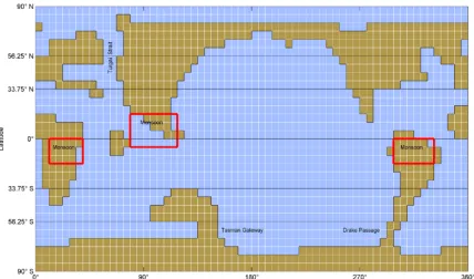
“Goldstein” is a 3-D frictional-geostrophic ocean model (Edwards and Marsh, 2005; Marsh et al., 2011), dynamically similar to classical GCMs, except that it neglects momen-tum advection and acceleration. Barotropic flow around the four continental islands (Fig. 1) is derived from linear con-straints that arise from integrating the depth-averaged mo-mentum equations.
Figure 1.Eocene palaeogeography and geographic areas used to determine simple metric values.
1979; Semtner Jr., 1976). Sea-ice dynamics are represented by diffusion and advection by surface currents.
“Ents” (Williamson et al., 2006) models vegetative and soil carbon densities, assuming a single plant functional type. Photosynthesis depends upon temperature (with a double-peaked response representing boreal and tropical forest), at-mospheric CO2concentration and soil moisture availability.
Self-shading is parameterised. Land surface albedo, moisture bucket capacity and surface roughness are parameterised in terms of the simulated carbon pool densities.
The computational efficiency of PLASIM-GENIE is achieved mainly through low spatial resolution (∼5◦) and, relative- to high-complexity Earth system models, simplify-ing assumptions in physical processes. These include, for instance, simplified parameterisations of radiative transport and convection in the atmosphere, the neglect of momentum transport in the ocean and the representation of all vegeta-tion as a single plant funcvegeta-tional type. Climate sensitivity, the response of the climate to a doubling of atmospheric CO2
concentration, including feedbacks, is an emergent property of the model.
3.2 Model configuration 3.2.1 Model grid
This study was designed before Lunt et al. (2017) presented their Deep-Time Model Intercomparison Project (DeepMIP) guidelines for model simulations of the latest Paleocene and early Eocene. However, our palaeogeography is based
on the high-resolution digital reconstruction of the early Eocene published by Herold et al. (2014) and which Lunt et al. (2017) recommended should be used as the standard for all palaeoclimate simulations within the DeepMIP frame-work. We have used the data set of Herold et al. (2014) as an initial configuration for the tectonic layout, topography and bathymetric boundary conditions in our study. We have reduced the resolution of the Eocene palaeogeography pro-vided by Herold et al. (2014) to a configuration of 64 lon-gitude×32 latitude cells, with each cell representing 5.625◦ in each orientation. Cells at high latitudes therefore repre-sent smaller land areas than cells at low latitudes. Our verti-cal resolution is 32 ocean depths and 10 atmospheric layers. We have incorporated the ocean gateway configurations dis-cussed in Sect. 2.2.1. The Turgai Strait is open in our config-uration and is the only connection between the Arctic Ocean and other oceans. The Drake Passage and Tasman Gateway are both closed.
The palaeogeography (Fig. 1) comprises four land masses: North (N.) America and Eurasia; Antarctica combined with South (S.) America and Australia; Africa; and India. Red rectangles in Fig. 1 indicate the boundaries of areas used to calculate simple metrics of centennially averaged seasonal precipitation, as empirical indicators of African, Asian and S. American monsoons.
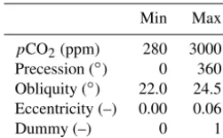
3.2.2 Forcing and other input parameters
Table 1.Uniform ranges for forcing and dummy parameters.
Min Max
pCO2(ppm) 280 3000 Precession (◦) 0 360 Obliquity (◦) 22.0 24.5 Eccentricity (–) 0.00 0.06
Dummy (–) 0 1
have constructed an ensemble of 50 model configurations, each with a unique set of forcing parameters comprising at-mospheric CO2, eccentricity (e), obliquity (ε) and precession
(ω), the angle on the Earth’s orbit around the Sun between the moving vernal equinox and the longitude of perihelion (Berger et al., 1993). When eis zero, the Earth’s distance from the Sun is constant at all points on the orbit, so there is no precessional effect. The magnitude of precessional effects is controlled by e, while phase is controlled by ω, so pre-cessional effects are commonly described by the precession index given byesinω. The precession index is at its maxi-mum value when perihelion occurs at the December solstice, its minimum value when perihelion is at the June solstice and has a value of 0.0 when perihelion is at either the March or September equinox. The only orbital parameter which alters the total annual solar radiation received by the Earth is e, although the range of variation is very small. We includee
andωas separate and independent forcing parameters, rather than combined as the precession index, or in the formecosω. An additional dummy parameter is included to test for pos-sible overfitting of relationships between forcing parameters and model output fields.
Although the maximum mass of CO2injected into the
at-mosphere during CIEs, and in particular the PETM, remains uncertain, there is broad agreement that the atmospheric con-centration of CO2did not exceed 3000 ppm (e.g. Gehler et
al., 2016) and that it did not fall below the pre-industrial level of 280 ppm at any time during the early Eocene. We allocate these values as the limits of a uniform range from which our ensemble of CO2values is selected.
Since the absolute astronomical timescale for the early Eocene has an uncertainty which is greater than the periods of the obliquity and precession cycles, and there remains dis-agreement as to which phases of the eccentricity cycles are related to CIEs, there are no combinations of the orbital forc-ing parameters which can be known a priori to be of greater importance in their effects on the Eocene climate, in general, and on their contributions to the initiation, duration and ter-mination of the CIEs in particular. We therefore select values of orbital parameters independently and from the full range of each parameter’s variation during the early Eocene.
To ensure the best coverage of the five-dimensional state space comprised of the four forcing parameters and the addi-tional dummy parameter in a limited number of model runs,
we apply the Latin hypercube method (McKay et al., 1979), a constrained Monte Carlo sampling scheme in which the range to be sampled for each variable is divided into non-overlapping intervals, and one value from each interval is randomly selected (Wyss and Jorgensen, 1998). This pro-vides adequate coverage of the state space more efficiently than can be achieved by a simple Monte Carlo sampling ap-proach (Rougier, 2007). The present study has been designed to facilitate direct comparison between the results for spe-cific ensemble members and their direct counterparts in a fu-ture study using the EMIC model GENIE-1 (Edwards and Marsh, 2005), which will include additional forcing parame-ters not used by this PLASIM-GENIE study. We have applied an iterative method to generate a pair of corresponding hy-percubes with 5 and 11 dimensions for the PLASIM-GENIE and GENIE-1 studies, respectively, in which the minimum Euclidean distance between any two points is maximised, and linear correlation between any two parameters is min-imised. We note that our selection of values forω, an angu-lar parameter, is from 0 to 360◦, treated as a linear range, with the consequence that the maximin criterion within the Latin hypercube algorithm is incorrectly calculated. How-ever, given the dimensionality of our experimental design, this is unlikely to result in a significant reduction in the ef-ficiency with which design points are distributed throughout the very sparsely populated state space. We draw readers’ at-tention to an approach presented by Bounceur et al. (2015), in which independent values ofesinω,ecosωandεare sam-pled, with rejection of absolute values ofesinωandecosω
which equal or exceed the maximum value ofe. This exper-imental design allows values ofeandωfor any design point to be identified by trigonometric analysis, while efficiently sampling the state space. Details of the steps taken to gener-ate the hypercubes are provided in Appendix A. The absolute value of ther correlation coefficient does not exceed 0.1 for any pair of input (forcing and dummy) parameters. Uniform ranges for each of the forcing parameters and the dummy pa-rameter are shown in Table 1, and the values applied in all 50 PLASIM-GENIE ensemble members are shown in Table 2.
The intensity of radiation emitted by the Sun has in-creased steadily over time, and we apply the linear model of Gough (1981) and select a solar constant of 1358.68 W m−2. We note that Lunt et al. (2017) have recommended that a modern value of 1361.0 W m−2should be applied to studies within the DeepMIP framework, in order to facilitate com-parison between simulations with modern and pre-industrial levels of CO2, and to offset the absence of elevated levels of
CH4.
3.2.3 Running the models
Table 2.Forcing factors and dummy values for each member in the ensemble. Precession is indicated byω, the angle between the moving vernal equinox and the longitude of perihelion.
Member (–) CO2(ppm) Eccentricity (–) Precession (◦) Obliquity (◦) Dummy (–)
1 975.6 0.0022 142.5 22.37 0.822
2 2418.7 0.0256 165.2 23.95 0.907
3 1259.4 0.0007 307.1 23.91 0.323
4 801.3 0.0163 270.4 23.50 0.276
5 1720.1 0.0559 206.7 23.82 0.402
6 327.1 0.0595 135.9 23.53 0.681
7 2937.7 0.0418 287.1 22.53 0.650
8 1200.3 0.0237 313.2 24.12 0.978
9 1420.7 0.0158 297.1 23.86 0.931
10 2157.6 0.0432 100.6 23.74 0.661
11 1791.7 0.0241 247.2 23.43 0.429
12 2369.0 0.0425 78.9 22.65 0.167
13 2502.9 0.0296 0.5 22.69 0.122
14 2149.2 0.0405 249.9 24.23 0.347
15 1061.7 0.0394 40.9 23.94 0.189
16 711.3 0.0199 274.6 22.08 0.913
17 1817.1 0.0578 291.4 23.08 0.888
18 722.1 0.0463 195.8 24.38 0.865
19 2988.5 0.0039 110.1 24.40 0.049
20 539.4 0.0251 212.5 23.29 0.234
21 450.6 0.0335 96.1 22.28 0.674
22 2700.1 0.0049 165.9 23.66 0.630
23 2025.4 0.0320 189.4 23.63 0.087
24 2268.7 0.0308 233.3 22.86 0.461
25 1447.2 0.0364 62.0 23.40 0.541
26 1168.3 0.0300 147.4 22.97 0.947
27 1317.6 0.0377 12.4 23.04 0.714
28 1639.5 0.0265 150.9 22.98 0.524
29 399.0 0.0589 262.7 23.46 0.028
30 2876.3 0.0411 203.0 22.05 0.608
31 2611.1 0.0170 54.3 22.84 0.746
32 2831.7 0.0564 187.2 23.72 0.696
33 1998.5 0.0372 278.8 24.19 0.805
34 1465.0 0.0439 38.9 23.50 0.376
35 1660.0 0.0109 85.3 22.88 0.896
36 2393.7 0.0587 127.9 24.27 0.191
37 286.3 0.0004 27.1 23.99 0.391
38 667.4 0.0509 116.5 22.71 0.569
39 2246.8 0.0450 317.4 22.90 0.103
40 2334.2 0.0096 294.7 23.61 0.532
41 2968.2 0.0346 329.8 22.51 0.314
42 768.2 0.0085 218.3 23.00 0.000
43 925.8 0.0450 327.2 24.32 0.753
44 384.5 0.0081 60.6 22.59 0.436
45 850.7 0.0551 322.9 23.21 0.459
46 1112.8 0.0150 356.7 23.27 0.579
47 1255.8 0.0116 212.2 22.31 0.487
48 1124.1 0.0530 343.7 22.40 0.065
49 2113.9 0.0276 9.9 22.19 0.856
representing both winter and summer seasons in both the Northern Hemisphere and Southern Hemisphere. Although model output includes time series of some fields and output values every 100 years, in this study, only the field values recorded at the end of the 1000 years of modelling are used for analysis of the results.
3.3 Analysis of model output
Comparison of the forcing parameters applied in the en-semble with the model output fields can be more efficiently achieved by reducing the dimensionality of the model out-put while retaining information on key components of the climate system.
3.3.1 Simple metrics
In studies of the Earth’s modern climate, it is recognised that the tropical–polar temperature difference (TPTD) influ-ences poleward energy flux, and the ocean–land temperature contrast (OLC) affects monsoon intensity (Jain et al., 1999; Karoly and Braganza, 2001; Peixoto and Oort, 1992). Al-though atmospheric circulation patterns in the early Eocene will have differed from those in the modern world, in se-lecting latitude regions to represent the TPTD, we adopt the approach of Abbot and Tziperman (2008), who configured their model of the Cretaceous climate with latitude ranges of 0–30, 30–60 and 60–90◦, the approximate boundaries of the Hadley, Ferrel and polar cells observed in the modern world (Peixoto and Oort, 1992). On our model grid in which each cell spans 5.625◦of latitude, for the purposes of deriv-ing scalar metrics, we define the tropical regions to be be-tween 0.0 and 33.75◦north and south, and the polar regions to be between 56.25 and 90◦north and south.
From the output values of air temperature in the lowest level of the atmosphere, weighted by grid cell area, we de-rive scalar values for each model run, of global annual mean air temperature (MAT), Northern Hemisphere and South-ern Hemisphere seasonality (mean area-weighted DJF–JJA temperature differences in the above-defined polar regions), TPTD for summer and winter in each hemisphere, and OLC for summer and winter in tropical and polar regions in each hemisphere.
Monsoons are related to seasonal variations in tropical and subtropical winds and precipitation (Trenberth et al., 2006). Wang and Fan (1999) noted that the choice of an index to denote monsoon behaviour in the modern world is difficult and arbitrary, with commonly applied indices based on aver-age summer precipitation, maximum summer precipitation, winter–summer difference in precipitation or wind circula-tion patterns within defined geographical areas. In this study, we derive simple scalar metrics to denote indices for mon-soons for Asia, Africa and South America by subtracting winter rainfall from summer rainfall, for defined geograph-ical regions, denoted in Fig. 1, and selected for their
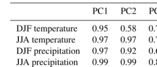
similar-Table 3. R2 correlation between PC scores from SVD and PC scores emulated with the linear models.
PC1 PC2 PC3
DJF temperature 0.95 0.58 0.75 JJA temperature 0.97 0.97 0.72 DJF precipitation 0.97 0.92 0.64 JJA precipitation 0.99 0.99 0.89
ity to monsoonal regions in the modern continental configu-ration.
3.3.2 Singular value decomposition, linear modelling and model emulation
We perform a singular value decomposition to identify the PCs and empirical orthogonal functions (EOFs) of temper-ature and precipitation fields in the full ensemble, although we note that climate variability may not be due to physical processes which vary orthogonally, and identification of PCs can be influenced by aspects of the experimental design. A detailed presentation of the use of this method in the analysis of climate data is given by Hannachi (2004).
We use the linear modelling method of Holden et al. (2015) to regress both the simple scalar metrics and the SVD reduced dimension model outputs onto the forcing pa-rameters. Values of the forcing parameters CO2,eandε(with
its very small angular range considered to be approximately linear) were normalised to the range [−1, 1] and combined with sinωand cosωto form 50-element column vectors rep-resenting the forcing factors. Each 2-D (32×64) result field for each ensemble member was unrolled to form a column vector of 2048 elements, comprising a single column within a 2048×50 matrix of full ensemble values.
SVD was applied to decompose the full ensemble matrix for each 2-D result field, providing a 2048×50 matrix of PCs, a 50×50 matrix of PC scores and a 50×50 matrix of diagonal values.
Figure 2.Ensemble temperature medians(a, c)and standard deviations(b, d)in DJF(a, b)and JJA(c, d).
Our emulator approach uses linear regression, rather than a Gaussian process (GP), and is therefore simpler than the methods applied by Bounceur et al. (2015) in a study of the response of the climate–vegetation system in interglacial conditions to astronomical forcing, and by Araya-Melo et al. (2015) in their study of the Indian monsoon in the Pleis-tocene. Unlike linear models, GP models are intrinsically stochastic and give a more accurate quantification of their own error in emulating the input data. However, GP models can become computationally demanding in high-dimensional space, and their results can be more difficult to interpret.
In order to analyse the results of each of our linear mod-els, we apply the method described in detail by Holden et al. (2015) to derive the main effects (Oakley and O’Hagan, 2004), which provide a measure of the variation in the linear model output due to each of the terms (first order, second or-der and cross products), or-derived from their coefficients, and total effects (Homma and Saltelli, 1996), which separate the effect of each forcing parameter on the variation in the model output. Although the forcing factors are all scaled within the range [−1, 1], the trigonometrical precession terms are not uniformly distributed across this range. We have therefore computed the variances of the first-order, second-order and cross-product terms directly for all parameters; rather than applying the respective approximations of 1/3, 1/9 and 4/45, we have applied these values as scaling factors in calculating the main effects and total effects.
4 Results
4.1 Model output – temperature and precipitation Analysis of the model results has focused on variation in surface air temperature and precipitation in both winter and summer in each hemisphere, although it should be noted that our experiment has not been designed such that mean val-ues in our ensemble output represent direct estimates of the Eocene climate mean. In the left column of Fig. 2, median temperatures at each grid cell for the full ensemble are plot-ted for DJF (Fig. 2a) and for JJA (Fig. 2c), with the standard deviations plotted in the right column column (Fig. 2b and d).
Ranges of median temperatures over land are greater than over the oceans, but TPTD is smaller in both seasons and both hemispheres than simulated in the modern world (see Fig. 2, Holden et al., 2016). It is apparent from the stan-dard deviation field that the tropical–polar temperature dif-ference varies substantially across the ensemble, particularly in northern winter. The temperature distributions are simi-lar to those of the 2240 ppm CO2 simulation of HC11,
re-garded as their “mid-to-late Eocene” analogue (they consider elevated CO2 as a proxy for all radiative forcing, including
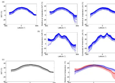
Figure 3.(a)Full ensemble distributions of mean latitude values of global annual mean sea surface temperature (SST), with mean latitude maritime surface air temperature in DJF and JJA.(b)Mean latitude continental surface air temperature in DJF and JJA.(c)Ensemble medians and 5 and 95 % percentiles of global annual mean SST and maritime surface air temperature in DJF (red) and JJA (blue).
in any of the 50 simulations in our study. Tropical temper-atures in excess of 35◦C were simulated in some cases, as in HC11, which they regarded as their “most troubling re-sult”, although they note observational data are currently in-sufficient to rule this out. Finally, we note that multi-model ensembles have found significant inter-model differences in-cluding, for instance, a 9◦C spread in global average temper-ature under the same CO2forcing (Lunt et al., 2012).
Quan-tification of model-related uncertainty is beyond the scope of the present study.
Full ensemble distributions of mean latitudinal distribu-tions of annual mean sea surface temperature (SST), with mean latitudinal distributions of maritime and continental surface air temperature in both DJF and JJA, are plotted in Fig. 3, together with ensemble medians and 5 and 95 % per-centiles of global annual mean SST and maritime surface air temperature in both DJF and JJA. The greater range of tem-peratures below rather than above median values reflects our use of a uniform range of CO2forcing values and the
loga-rithmic response of temperature to increasing CO2
concen-tration. There is substantial variation of mean temperature across the ensemble, around 20◦over land, but the tempera-ture offset varies little with latitude outside of polar regions where snow and ice greatly reduce winter temperatures in the colder simulations. The variation in TPTD across the
ensem-ble thus appears to be essentially driven by the strength of snow and ice albedo feedbacks.
Our ensemble distributions of sea and air temperatures are in broad agreement with the values from the Eocene model studies compared by Lunt et al. (2012), hereafter L12, and with the tables of marine and terrestrial proxy data compiled by L12 and HC11, covering the early Eocene, and including some records from the very latest Paleocene but not includ-ing the PETM. Our palaeogeography specifically represents the early Eocene, but our range of CO2 and orbital inputs
is more representative of the variation in forcing across the whole era. L12 have summarised variations of SST with lati-tude from their proxy data set, in their Fig. 1, including large error bars representing uncertainty which they attribute to as-sumptions about seawater chemistry, possible non-analogous behaviour between modern and ancient systems, and uncer-tainty in calibrations of relationships between proxy data and properties of the palaeoclimate. Our median values of SST are close to the median estimates of SST in L12 at midlati-tudes, and well within the uncertainty indicated by error bars at high latitudes.
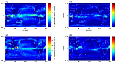
Figure 4.Ensemble precipitation medians(a, c)and standard deviations(b, d)in DJF(a, b)and JJA(c, d).
day: Africa and S. America in DJF, and southeast (S.E.) Asia in JJA.
4.2 Simple metrics
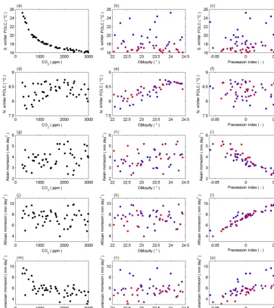
In Figs. 5 and 6, CO2, obliquity (ε) and precession
in-dex (esinω) are plotted against MAT, northern seasonality, northern winter TPTD and northern summer TPTD (Fig. 5), and southern winter polar OLC, northern winter polar OLC, Asian monsoon index, African monsoon index and the S. American (hereafter referred to as “American”) monsoon in-dex (Fig. 6). Subplots for obliquity and precession inin-dex in Figs. 5 and 6 denote the CO2 level on a continuous colour
scale. The dominant effect of CO2on MAT and northern
sea-sonality is apparent in Fig. 5, and it can also be seen that CO2 strongly affects the northern TPTD in the winter, but
not in the summer, when the combined influence of obliquity and precession index is discernible, suggesting that temper-ature proxies with seasonal bias may have a significant or-bital imprint. The plot of atmospheric CO2against northern
winter TPTD shows a change in gradient at approximately 1000 ppm CO2 and 32◦C. This may be related to the
log-arithmic dependence of radiative forcing on CO2
concentra-tion, the disappearance of ice above some threshold level and a minimum level of land surface albedo related to maximum vegetation cover. A possible sea-ice-related threshold mech-anism influencing both SST and maritime air temperature in high northern latitudes may be observed in Fig. 3, and this is strongly associated with the increase in northern winter TPTD at low CO2levels. Zeebe et al. (2017) have analysed
a high-resolution benthic isotope record covering the late Palaeocene – early Eocene and have concluded that orbitally paced cycles are unlikely to have been driven by high-latitude mechanisms, but our PLASIM-GENIE modelling suggests that while northern TPTD is not orbitally paced in the winter, being controlled by CO2, it is orbitally paced in the summer,
by a combination of obliquity and precession.
It can be observed in Fig. 6 that there is strong corre-lation between CO2 and southern winter polar OLC. The
African and Asian monsoon indices are both correlated with the precession index, a well-established feature of Quater-nary records (e.g. Cruz et al., 2005). The American monsoon index is fairly strongly correlated with the precession index at high levels of CO2and negatively correlated with CO2at low
levels of CO2. In each of the other examples, there is no
ap-parent correlation between the simple metric and two of the three forcing factors. We have selected these simple metrics with visible correlations to the forcing parameters for further analysis with the linear modelling and emulation methods. Total effects on the simple metrics have been calculated for each of the forcing parameters, with eccentricity and preces-sion considered separately, rather than combined within the precession index, and are shown in Table 4.
The total effects of CO2on MAT, northern winter TPTD
Figure 5.Correlation between three forcing factors (CO2, obliquity and precession index; in columns from left to right) and the simple
metrics (MAT, northern seasonality, northern winter tropical–polar temperature difference and northern summer tropical–polar temperature difference; in rows from top to bottom). CO2is plotted in colour in the obliquity and precession plots (blue is low; red is high).
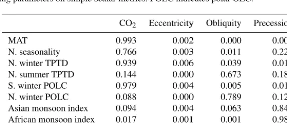
Table 4.Total effects of forcing parameters on simple scalar metrics. POLC indicates polar OLC.
CO2 Eccentricity Obliquity Precession
MAT 0.993 0.002 0.000 0.005
N. seasonality 0.766 0.003 0.011 0.220
N. winter TPTD 0.939 0.006 0.039 0.017
N. summer TPTD 0.144 0.000 0.673 0.183
S. winter POLC 0.979 0.004 0.005 0.012
N. winter POLC 0.088 0.000 0.789 0.122
Asian monsoon index 0.094 0.004 0.063 0.840 African monsoon index 0.017 0.001 0.001 0.981 American monsoon index 0.490 0.004 0.020 0.486
high (> 0.65), providing quantitative confirmation of the cor-relations visible in Figs. 5 and 6.
4.3 Climate sensitivity and mean air temperature
Figure 7 shows the relationship between CO2(plotted on a
logarithmic scale) and MAT, with an abrupt change of gra-dient clearly visible at a CO2 concentration of 1000 ppm.
val-Figure 6.Correlation between three forcing factors (CO2, obliquity and precession index; in columns from left to right) and the simple
metrics (southern winter polar OLC, northern winter polar OLC, Asian monsoon index, African monsoon index and the S. American – hereafter referred to as “American” – monsoon index; in rows from top to bottom). CO2is plotted in colour in the obliquity and precession plots (blue is low; red is high).
ues for a doubling of CO2concentration at CO2levels below
1000 ppm and at CO2 levels above 1000 ppm, of 4.36 and
2.54◦C, respectively. We note that our modelled values of carbon in vegetation in the ENTS module remain low out-side of the tropics at low CO2 concentration, but as CO2
concentration increases, land areas at higher latitudes reach maximum values of carbon in vegetation, with all land areas showing no further capacity for increased carbon in vege-tation at an atmospheric concentration of ∼1000 ppm. The increase in land vegetation cover, with corresponding reduc-tion in albedo, acts as a positive feedback to rising
tempera-ture caused by increasing CO2, but this feedback mechanism
ceases to operate when all available land is at its maximum vegetation capacity, with a consequent reduction in the cli-mate sensitivity.
For a pre-industrial atmospheric CO2 concentration of
280 ppm, the value of MAT indicated by our results for our early Eocene palaeogeography is 14.0◦C. Holden et al. (2016) applied an identically configured PLASIM-GENIE to a modern geography, and their results show that with a pre-industrial CO2concentration, the model climate sensitivity is
Figure 7.Mean air temperature plotted against CO2on a logarithmic scale, with regression lines plotted for CO2< 1000 ppm (blue) and
CO2> 1000 ppm (red), with climate sensitivities for a doubling of CO2from both of the regressions.
Our results also indicate values of global MAT for dou-ble and 4 times the pre-industrial levels of CO2of 18.5 and
22.5◦C, respectively; both these values are within the ranges of results for land near-surface air temperature in the mod-elling studies compared by L12 and shown in their Fig. 2b.
4.4 Singular value decomposition
Figure 8 shows the first three PCs of surface air temperature in DJF and JJA, with the percentages of temperature variation explained by each PC. Each of these plots illustrates the PC scaled by the standard deviation of the PC scores, thereby re-flecting the variability across the ensemble. Note the variable scales for each of the subplots. In both DJF and JJA, PC1 ex-plains over 95 % of the variance, with TPTD clearly visible in both hemispheres in DJF but apparent only in the Southern Hemisphere in JJA. OLC is apparent in the plots of PC1 in both DJF and JJA. OLC is discernible in PC2 for DJF tem-perature, which explains 2.4 % of variance, but less apparent, at least in the Southern Hemisphere, for JJA temperatures, in which PC2 explains 2.6 % of the variance. For temperature in both DJF and JJA, PC3 explains less than 1 % of the vari-ance, with some indication of TPTD and OLC in DJF, but only of weak OLC at high latitudes in JJA. It is worth noting that even though lower-order PCs explain small percentages of global variances, these PCs are generally associated with specific regions where they are comparably important to the first PC.
In their presentation of the SVD method applied in this study, Holden et al. (2015) investigated the effects of orbital parameters on the Earth’s climate in the present day but with-out including CO2as a forcing parameter in their ensemble,
and found that obliquity had a dominant effect on the PC
Table 5.R correlation values for PC scores for temperature and precipitation in DJF and JJA. Values whereR2≥0.5 are shown in bold.
DJF precipitation
PC1 PC2 PC3
PC1 0.993 −0.004 −0.080 DJF temperature PC2 −0.067 −0.364 −0.864 PC3 0.005 0.783 −0.354
JJA precipitation
PC1 PC2 PC3
PC1 0.976 0.091 0.157 JJA temperature PC2 0.098 −0.947 0.082 PC3 −0.180 −0.049 0.795
score of annual average surface air temperature. In our study of the Eocene climate, CO2is strongly correlated with
north-ern seasonality (Fig. 5), and obliquity is weakly correlated with TPTD in JJA (Fig. 5) and with OLC in DJF (Fig. 6). The first three PCs of precipitation in DJF and JJA are shown in Fig. 9. PC1 explains approximately 55 % of the variance in both seasons, with PC2 and PC3 explaining over 20 and over 5 %, respectively, in both seasons. In both PC2 and PC3, ar-eas of high sar-easonal contrast appear to correspond to arar-eas which experience monsoons in the modern world.
Figure 8.The first three principal components of DJF temperature(a)and JJA temperature(b). Percentages of variance explained by each principal component are shown above each plot.
Figure 9.The first three principal components of DJF precipitation(a)and JJA precipitation(b). Percentages of variance explained by each principal component are shown above each plot.
cycle in response to warming. Similar considerations reveal connections between lower-order PC scores, though we note that the second (third) component of DJF temperature is as-sociated with the third (second) component of DJF precipita-tion. In order to address the drivers of these modes, we first consider the correlation coefficients,r, between forcing fac-tors and the PC scores, shown in Table 6. These demonstrate that for each output there is a mode of variability driven by CO2and another mode driven by precession, suggesting they
reflect global warming (and associated hydrological strength) and precessional forcing of the monsoon system.
There is strong correlation (r2> 0.5) between CO2and the
first PC scores of temperature in DJF and JJA. There are also strong correlations between precession index and the third
PC scores for DJF temperature, and between precession in-dex and the second PC scores for JJA temperature.
CO2is strongly correlated with the first PC scores of
in-Table 6. R correlation values for forcing factors and PC scores. Values whereR2≥0.5 are shown in bold.
CO2 Precession Obliquity
index
PC1 −0.859 −0.018 −0.057 DJF temperature PC2 0.381 −0.087 −0.354 PC3 0.038 −0.924 0.311
PC1 −0.899 0.178 −0.066 JJA temperature PC2 −0.018 −0.875 0.362 PC3 0.342 0.056 −0.239
PC1 −0.867 0.003 −0.025 DJF precipitation PC2 −0.198 −0.82 0.044 PC3 −0.278 0.465 0.164
PC1 −0.953 0.065 0.008 JJA precipitation PC2 −0.07 0.96 −0.131
PC3 0.219 0.191 −0.029
coming solar radiation associated with increased cloud cover and surface evaporation.
4.5 Linear modelling and emulation
The relationships between the forcing parameters (with pre-cession expressed as both sinω and cosω) and the simple metrics, and between the forcing parameters and the PC scores of 2-D fields, derived through linear modelling, in-clude first- and second-order terms of forcing factors, to-gether with products of forcing factors. In all cases, most of the main effects are confined to the first-order terms, and in no case does eccentricity have a significant effect indepen-dently of either of the precession terms. All significant effects of the precession terms are accompanied by a small effect of eccentricity.
In Fig. 10, we plot the main effects of the forcing parame-ters on the first three PCs of temperature and precipitation for DJF. Figure 11 shows the main effects of the forcing param-eters on the first three PCs of temperature and precipitation plotted for JJA.
In both seasons, PC1 for temperature and precipitation can be almost entirely explained by CO2, reinforcing the
earlier conclusion that these describe a connected mode, global warming with associated effects on the hydrological cycle. The main effects also suggest connections between the modes of variability of temperature and precipitation in lower-order components. In both seasons, and apparent in both variables, there is a mode that is driven by precession; we interpret this as a monsoon signal, given precessional forcing and spatial patterns of rainfall that are characteris-tic of modern monsoons (Figs. 8 and 9). In JJA, this is the second component of both variables. The mode is associated with precipitation variability of∼2.5 mm day−1and temper-ature variability of∼3◦C, with increased precipitation
asso-Figure 10. Main effects of forcing parameters on the first three principal components of DJF temperature(a)and DJF precipitation (b).
ciated with a surface air cooling (note the negative correla-tion in Table 3, so that positive change in one field is asso-ciated with negative change in the other). In both cases, the local magnitude of variability is comparable to that driven by CO2. In DJF, the precessional signal is again apparent in the
second mode of precipitation but the third mode of tempera-ture. This mode is notable in that it drives changes in simu-lated precipitation over east Africa (5 mm day−1) that exceed
CO2-driven variability. The remaining modes are more
com-plex and may not represent a clear mode of variability that can be straightforwardly attributed. For instance, the third-order mode of JJA temperature is driven by an interaction between CO2 and obliquity, but in precipitation can be
ex-plained by a combination of precession and CO2.
All of the terms in the linear models derived from the forcing factors and the three monsoon indices are shown in Table 7. The Asian and African models are dominated by precession terms, roughly equally distributed between first-order sin(ω) and the cross product of e and sin(ω), with|sin(ω)|being approximately 5 and 8 times larger than |cos(ω)|for the Asian and African models, respectively. The American model identifies significant influence of CO2, in
Figure 11. Main effects of forcing parameters on the first three principal components of JJA temperature (a) and JJA precipita-tion(b).
Table 7.Linear models derived from normalised forcing functions and monsoon indices.
Terms Asia Africa America
Intercept −0.096 0.200 −0.273 CO2 0.187 −0.089 −0.422
ε 0.189 0.027 0.065
e 0.049 −0.091 −0.070
sin(ω) −0.577 0.510 0.309 cos(ω) −0.114 −0.064 −0.105
CO22 – 0.150 0.278
e2 – −0.115
e×sin(ω) −0.468 0.501 0.240 CO2×sin(ω) −0.214 0.215 −0.085 ε×sin(ω) – −0.069 −0.071
e×cos(ω) −0.100 – –
sin(ω)×cos(ω) 0.118 – –
ε×cos(ω) – −0.121 –
CO2×ε 0.121 – –
CO2×cos(ω) – 0.098 –
CO2×e – 0.096 –
We apply these linear models as emulators to estimate val-ues of monsoon indices corresponding to the full range of precession (ω), with eccentricity fixed at its high limit of 0.06, low and high values of CO2(300 and 3000 ppm), and
low and high values of obliquity (22.0 and 24.5◦). Precession index (esinω) and emulated values of the Asian, African and American monsoon indices for all four combinations of high and low CO2and obliquity are plotted in Figs. 12, 13 and
14, respectively. The elliptical form of each of the plots is controlled by model terms which include cos(ω) and iden-tify seasonal processes in the development of the monsoons.
excluded, generates points on a straight line between each apex of the ellipses generated by the full emulator. In each of the 12 plots in Figs. 12–14,ωincreases anticlockwise from a value of 0◦in the centre of the lower arc of the ellipse (with perihelion at the March equinox), through a value of 180◦in the centre of the upper arc (with perihelion at the September equinox). Relationships between the precession index and the monsoon indices which are visually suggested in Fig. 6 are shown with clear structure in Figs. 12, 13 and 14. In each of the monsoon areas, the highest levels of precipitation oc-cur when perihelion coincides with the summer solstice, in June for the Asian monsoon in the Northern Hemisphere and in December for the African and American monsoons in the Southern Hemisphere. For the Asian and African monsoons, precipitation is increased by high CO2, particularly when
perihelion is at the summer solstice, but for the American monsoon, high CO2decreases precipitation. The plots of the
emulated African and American monsoons (Figs. 13 and 14) show the lowest and highest degrees of non-stationarity, re-spectively, due to the relative magnitude of the cos(ω) terms in the linear models.
5 Summary and conclusions
Our ensemble of 50 model runs of the EMIC PLASIM-GENIE has used an early Eocene palaeogeography incorpo-rating recent understanding of the configuration of the con-tinents and ocean gateways, with climate forcing by a ran-domly selected combination of atmospheric GHG emissions and orbital parameters for each model run. Relationships be-tween forcing parameters and scalar summaries of model re-sults have been derived through linear modelling.
Given the input range of CO2, our results show that, at
the global scale, variability in patterns of surface air tem-perature is strongly dominated by a single mode of variation with a strong imprint of TPTD, focused in northern winter, that is entirely controlled by CO2(> 95 % variance in both
seasons). We note, however, that regions under the influence of monsoon systems exhibit precession-driven temperature variability that is comparable in magnitude to the variabil-ity driven by CO2(in large part, the high proportion of
vari-ance explained by the CO2 mode arises because the signal
is global). In contrast to the unimodal dominance of CO2on
the modelled global temperature fields, precipitation shows a somewhat more nuanced response. The first mode of pre-cipitation, while still controlled entirely by CO2, is much less
dominant (maximum 57 % variance in DJF cf 21 % for PC2). In the second and third spatial modes of precipitation vari-ability, CO2is still important, but no more so than orbital
pa-rameters, with PC2 controlled more strongly by precession index.
Figure 12.Emulated values of the Asian monsoon index, for the full range of the precession index (esinω), at low and high values of CO2
and obliquity (ε).
of large variation in atmospheric CO2, variation in obliquity
accounts for well over half of the variation in high northern latitude ocean–land temperature contrast, and the variation in precession is the dominant influence on seasonal variation in precipitation in tropical Africa and Asia, and combines with CO2 to influence seasonal precipitation in tropical N.
and S. America. Our results strongly suggest the presence of monsoons in the early Eocene, but these climatic features would have developed without the effects of orography and high-altitude plateau heating which are important factors in the modern south Asian monsoon (Boos and Kuang, 2010).
We note that the relative amplitude of the CO2-driven
modes depends critically on the actual amplitude of CO2
variability in the period of interest. While the ranges for or-bital parameters are well defined, this is less true of CO2
vari-ability over the Eocene. If atmospheric CO2remained within
a narrower range throughout the period, for example, in the range 700 to 1800 ppm, indicated for the early Eocene by Anagnostou et al. (2016) in a recent study using boron iso-topes, then outside of short-lived hyperthermals, the relative influence of CO2 and orbital inputs might have been more
evenly balanced. Our modelling results suggest that climate sensitivity is state dependent, with a value of 4.36◦C in a low CO2state and 2.54◦C in a high CO2state, due to a
posi-tive feedback mechanism in which albedo reduces as
vegeta-tion increases to its maximum value when CO2concentration
reaches 1000 ppm.
We have demonstrated that emulators derived from linear modelling of the PLASIM-GENIE ensemble results can be used as a rapid and efficient method of estimating climate conditions from any set of forcing parameters, without the need for further deployment of the EMIC.
PLASIM-GENIE is to our knowledge the most sophisti-cated climate model that has been applied to an ensemble of Eocene simulations, but we note that increasing com-puting power is now enabling ensembles of simulations with moderately higher resolution models, such as HadCM3 (3.75◦×2.5◦) (e.g. Araya-Melo et al., 2015; Lord et al., 2017), to be run, although with some limitation in the model years in each simulation. It will never be possible to apply state-of-the-art climate models to large ensembles because, given the continual striving for the highest possible reso-lution, single simulations with such models will always be at the limits of what is practicable with available comput-ing power. EMICs therefore have an important role in fur-thering our understanding of past, present and future climate systems, and in the rapid identification of influencing factors and modes of response which may be targeted for study by slower but more powerful models.
pa-Figure 13.Emulated values of the African monsoon index, for the full range of the precession index (esinω), at low and high values of CO2
and obliquity (ε).
rameters can exert significant climatic influence, particularly in regard to tropical temperature and precipitation, and they should not be ignored in modelling studies of climates of the past.
This study has been designed together with a future study us-ing the EMIC model GENIE-1 (Edwards and Marsh, 2005). The GENIE-1 model will use all four of the forcing parame-ters and the dummy parameter, used in the present study, to-gether with an additional six forcing parameters not used by the PLASIM-GENIE study. For PLASIM-GENIE, we have run 50 simulations with five parameters, while in GENIE-1 we will run 100 simulations with 11 parameters, so that the number of runs in each ensemble is approximately 10 times the input dimension (Loeppky et al., 2012).
The overall design for both studies is based on a maximin Latin hypercube with 100 rows and 11 columns produced by repeatedly invoking thelhsdesignfunction in MATLAB (MathWorks), with the command
hyperCube=lhsdesign(100, 11,
“criterion”, “maximin”, “iterations”,100) to select from 100 iteratively generated hypercubes the one which best fits the maximin criterion, i.e. where the minimum Euclidian distance between points in hyperspace is at a maxi-mum. This MATLAB command is repeated until the absolute value of correlation between columns falls below a selected value, or until a selected number of attempts has been made. The ability of this “brute force” approach to produce a hyper-cube which satisfies the maximin criterion, with the required low correlation between columns, decreases rapidly with an increasing number of columns and a decreasing target cor-relation, but in several minutes it can generate a hypercube with 100 rows, each representing a design point for an en-semble member, and 11 columns, each representing a forc-ing or dummy parameter, with correlation between any two parameters not exceeding 0.1.
We then modify the overall design by first picking a sub-set of 50 of the 100 design points to give good coverage of the PLASIM-GENIE subspace. We randomly select an ini-tial point and iteratively select from the remainder, with-out replacement, the point which provides the largest in-crease in the number of populated sectors across all the two-dimensional projections of PLASIM-GENIE parameter space defined by dividing each two-dimensional subspace into 6×6 equal sectors.
11 parameter values.
Copying the template and discarding the six parameters which are only used in the GENIE-1 ensemble yields the final hypercube design for the PLASIM-GENIE ensemble, comprising 50 sets of five parameters.
A second copy of the template forms the top half of the GENIE-1 hypercube, and the bottom half is partially con-structed by duplicating only the five PLASIM-GENIE rameters from the first 50 rows, with the remaining six pa-rameters determined by choosing a previously unselected point, without replacement, from the initial 100×11 hyper-cube that maximises the Euclidean distance between the pair of points in the subspace of the remaining six parameters.
Author contributions. JK and PH designed and prepared the en-semble configurations and analysed the model outputs with advice from NE. JK prepared the paper with contributions from both co-authors.
Competing interests. The authors declare that they have no con-flict of interest.
Acknowledgements. The authors gratefully acknowledge support from NERC, with funding for project NE/K006223/1. We are very grateful to the reviewers are Michel Crucifix and David De Vleeschouwer, and to the editor Arne Winguth, for their thorough and constructive comments which have helped to improve the manuscript.
Edited by: Arne Winguth
Reviewed by: Michel Crucifix and David De Vleeschouwer
References
Abbot, D. S. and Tziperman, E.: A high-latitude convective cloud feedback and equable climates, Q. J. Roy. Meteor. Soc., 134, 165–185, https://doi.org/10.1002/qj.211, 2008.
Akaike, H.: A new look at the statistical model identification, IEEE T. Automat. Contr., 19, 716–723, 1974.
Akhmetiev, M. A., Zaporozhets, N. I., Benyamovskiy, V. N., Alek-sandrova, G. N., Iakovleva, A. I., and Oreshkina, T. V.: The Pale-ogene history of the Western Siberian seaway – A connection of the Peri-Tethys to the Arctic Ocean, Austrian J. Earth Sci., 105, 50–67, 2012.
Anagnostou, E., John, E. H., Edgar, K. M., Foster, G. L., Ridg-well, A., Inglis, G. N., Pancost, R. D., Lunt, D. J., and Pear-son, P. N.: Changing atmospheric CO2 concentration was the
primary driver of early Cenozoic climate, Nature, 533, 380–384, https://doi.org/10.1038/nature17423, 2016.
Araya-Melo, P. A., Crucifix, M., and Bounceur, N.: Global sensitiv-ity analysis of the Indian monsoon during the Pleistocene, Clim. Past, 11, 45–61, https://doi.org/10.5194/cp-11-45-2015, 2015. Aubry, M.-P., Ouda, K., Dupuis, C., Berggren, W. A., and
Couver-ing, J. A. V.: The Global Standard Stratotype-section and Point (GSSP) for the base of the Eocene Series in the Dababiya section (Egypt), Episodes, 30, 271–286, 2007.
Backman, J., Jakobsson, M., Frank, M., Sangiorgi, F., Brinkhuis, H., Stickley, C., O’Regan, M., Løvlie, R., Pälike, H., Spofforth, D., Gattacecca, J., Moran, K., King, J., and Heil, C.: Age model and core-seismic integration for the Cenozoic Arctic Coring Expedi-tion sediments from the Lomonosov Ridge, Paleoceanography, 23, 1–15, https://doi.org/10.1029/2007PA001476, 2008. Barker, P. and Burrell, J.: The opening of Drake passage, Mar. Geol.,
25, 15–34, 1977.
Berger, A., Loutre, M. F., and Tricot, C.: Insolation and Earth’s or-bital periods, J. Geophys. Res.-Atmos., 98, 10341–10362, 1993. Boos, W. R. and Kuang, Z.: Dominant control of the South Asian monsoon by orographic insulation versus plateau heating, Na-ture, 463, 218–222, https://doi.org/10.1038/nature08707, 2010.
Bounceur, N., Crucifix, M., and Wilkinson, R.: Global sensitivity analysis of the climate–vegetation system to astronomical forc-ing: an emulator-based approach, Earth Syst. Dynam., 6, 205– 224, https://doi.org/10.5194/esd-6-205-2015, 2015.
Burnham, K. P. and Anderson, D. R.: Model selection and mul-timodel inference: a practical information-theoretic approach, Springer, New York, 2003.
Carmichael, M. J., Lunt, D. J., Huber, M., Heinemann, M., Kiehl, J., LeGrande, A., Loptson, C. A., Roberts, C. D., Sagoo, N., Shields, C., Valdes, P. J., Winguth, A., Winguth, C., and Pan-cost, R. D.: A model–model and data–model comparison for the early Eocene hydrological cycle, Clim. Past, 12, 455–481, https://doi.org/10.5194/cp-12-455-2016, 2016.
Chen, Z., Ding, Z., Yang, S., Zhang, C., and Wang, X.: Increased precipitation and weathering across the Paleocene-Eocene ther-mal maximum in central China, Geochem. Geophy. Geosy., 17, 2286–2297, https://doi.org/10.1002/2016GC006333, 2016. Cruz, F. W., Burns, S. J., Karmann, I., Sharp, W. D., Vuille, M.,
Cardoso, A. O., Ferrari, J. A., Silva Dias, P. L., and Viana, O.: Insolation-driven changes in atmospheric circulation over the past 116,000 years in subtropical Brazil, Nature, 434, 63–66, https://doi.org/10.1038/nature03365, 2005.
Cui, Y., Kump, L. R., Ridgwell, A. J., Charles, A. J., Junium, C. K., Diefendorf, A. F., Freeman, K. H., Urban, N. M., and Harding, I. C.: Slow release of fossil carbon during the Palaeocene-Eocene Thermal Maximum, Nat. Geosci., 4, 481– 485, https://doi.org/10.1038/NGEO1179, 2011.
Dickens, G. R.: Down the rabbit hole: Toward appropriate discus-sion of methane release from gas hydrate systems during the Paleocene-Eocene thermal maximum and other past hyperther-mal events, Clim. Past, 7, 831–846, https://doi.org/10.5194/cp-7-831-2011, 2011.
Dickson, A. J., Cohen, A. S., and Coe, A. L.: Seawater oxygenation during the Paleocene-Eocene thermal maximum, Geology, 40, 639–642, https://doi.org/10.1130/G32977.1, 2012.
Dunkley Jones, T., Lunt, D. J., Schmidt, D. N., Ridgwell, A., Sluijs, A., Valdes, P. J., and Maslin, M.: Climate model and proxy data constraints on ocean warming across the Paleocene– Eocene Thermal Maximum, Earth-Sci. Rev., 125, 123–145, https://doi.org/10.1016/j.earscirev.2013.07.004, 2013.
Edwards, N. R. and Marsh, R.: Uncertainties due to transport-parameter sensitivity in an efficient 3-D ocean-climate model, Clim. Dynam., 24, 415–433, https://doi.org/10.1007/s00382-004-0508-8, 2005.
Exon, N. F., Kennett, J. P., and Malone, M. J.: Leg 189 synthesis: Cretaceous–Holocene history of the Tasmanian Gateway, in: Pro-ceedings of the Ocean Drilling Program, Scientific Results, 189, edited by: Exon, N. F., Kennett, J. P., and Malone, M. J., Ocean Drilling Program, College Station, TX 2004.
Fraedrich, K.: A suite of user-friendly global climate mod-els: hysteresis experiments, Eur. Phys. J. Plus, 127, 1–9, https://doi.org/10.1140/epjp/i2012-12053-7, 2012.
Fraedrich, K., Kirk, E., Luksch, U., and Lunkeit, F.: The portable university model of the atmosphere (PUMA): Storm track dy-namics and low-frequency variability, Meteorol. Z., 14, 735–745, https://doi.org/10.1127/0941-2948/2005/0074, 2005.
Gehler, A., Gingerich, P. D., and Pack, A.: Temperature and atmospheric CO2 concentration estimates through the
https://doi.org/10.1073/pnas.1518116113, 2016.
Gibbs, S. J., Bown, P. R., Sessa, J. A., Bralower, T. J., and Wil-son, P. A.: Nannoplankton extinction and origination across the Paleocene-Eocene thermal maximum, Science, 314, 1770–1773, 2006.
Hannachi, A.: A primer for EOF analysis of climate data, University of Reading, Reading, 2004.
Herold, N., Buzan, J., Seton, M., Goldner, A., Green, J., Müller, R., Markwick, P., and Huber, M.: A suite of early Eocene (∼55 Ma) climate model boundary conditions, Geosci. Model Dev., 7, 2077–2090, https://doi.org/10.5194/gmd-7-2077-2014, 2014. Hibler III, W.: A dynamic thermodynamic sea ice model, J. Phys.
Oceanogr., 9, 815–846, 1979.
Hilgen, F. J., Kuiper, K. F., and Lourens, L. J.: Evalu-ation of the astronomical time scale for the Paleocene and earliest Eocene, Earth Planet. Sc. Lett., 300, 139–151, https://doi.org/10.1016/j.epsl.2010.09.044, 2010.
Hinnov, L. A. and Hilgen, F. J.: Chapter 4 – Cyclostratigraphy and Astrochronology, in: The Geologic Time Scale 2012, edited by: Gradstein, F. M., Ogg, J. G., Schmitz, M. D., and Ogg, G. M., Elsevier, Boston, 2012.
Holden, P., Edwards, N., Garthwaite, P., Fraedrich, K., Lunkeit, F., Kirk, E., Labriet, M., Kanudia, A., and Babonneau, F.: PLASIM-ENTSem v1. 0: a spatio-temporal emulator of future climate change for impacts assessment, Geosci. Model Dev., 7, 433–451, https://doi.org/10.5194/gmd-7-433-2014, 2014.
Holden, P. B., Edwards, N. R., Garthwaite, P. H., and Wilkin-son, R. D.: Emulation and interpretation of high-dimensional climate model outputs, J. Appl. Stat., 42, 2038–2055, https://doi.org/10.1080/02664763.2015.1016412, 2015. Holden, P. B., Edwards, N. R., Fraedrich, K., Kirk, E., Lunkeit,
F., and Zhu, X.: PLASIM–GENIE v1.0: a new intermedi-ate complexity AOGCM, Geosci. Model Dev., 9, 3347–3361, https://doi.org/10.5194/gmd-9-3347-2016, 2016.
Homma, T. and Saltelli, A.: Importance measures in global sensi-tivity analysis of nonlinear models, Reliab. Eng. Syst. Safety, 52, 1–17, 1996.
Huber, M.: Progress in greenhouse climate modeling, in: Recon-structing Earth’s Deep-Time Climate – The State of the Art in 2012, edited by: Ivany, L. C. and Huber, B. T., The Paleontolog-ical Society, Boulder, CO, 2012.
Huber, M. and Caballero, R.: The early Eocene equable climate problem revisited, Clim. Past, 7, 603–633, https://doi.org/10.5194/cp-7-603-2011, 2011.
Jain, S., Lall, U., and Mann, M. E.: Seasonality and interannual variations of Northern Hemisphere temperature: Equator-to-pole gradient and ocean-land contrast, J. Clim., 12, 1086–1100, 1999. Jenkyns, H. C.: Geochemistry of oceanic anoxic events, Geochem. Geophy. Geosy., 11, 1–30, https://doi.org/10.1029/2009GC002788, 2010.
Jones, P. D. and Mann, M. E.: Climate over past millennia, Rev. Geophys., 42, 1–42, 2004.
Karoly, D. J. and Braganza, K.: Identifying global climate change using simple indices, Geophys. Res. Lett., 28, 2205–2208, 2001. Kennett, J. and Stott, L.: Abrupt deep-sea warming, palaeoceanographic changes and benthic extinctions at the end of the Palaeocene, Nature, 353, 225–229, https://doi.org/10.1038/353225a0, 1991.
new orbital solution for the long-term motion of the Earth, As-tron. Astrophys., 532, A89, 1–15, https://doi.org/10.1051/0004-6361/201116836, 2011.
Lauretano, V., Littler, K., Polling, M., Zachos, J. C., and Lourens, L. J.: Frequency, magnitude and character of hyperthermal events at the onset of the Early Eocene Climatic Optimum, Clim. Past, 11, 1313–1324, https://doi.org/10.5194/cp-11-1313-2015, 2015. Laurin, J., Meyers, S. R., Galeotti, S., and Lanci, L.:
Fre-quency modulation reveals the phasing of orbital eccentric-ity during Cretaceous Oceanic Anoxic Event II and the Eocene hyperthermals, Earth Planet. Sc. Lett., 442, 143–156, https://doi.org/10.1016/j.epsl.2016.02.047, 2016.
Loeppky, J. L., Sacks, J., and Welch, W. J.: Choosing the sample size of a computer experiment: A practical guide, Technometrics, 51, 366–376, 2012.
Lord, N. S., Crucifix, M., Lunt, D. J., Thorne, M. C., Bounceur, N., Dowsett, H., O’Brien, C. L., and Ridgwell, A.: Emu-lation of long-term changes in global climate: Application to the late Pliocene and future, Clim. Past, 13, 1539–1571, https://doi.org/10.5194/cp-13-1539-2017, 2017.
Lourens, L. J., Sluijs, A., Kroon, D., Zachos, J. C., Thomas, E., Röhl, U., Bowles, J., and Raffi, I.: Astronomical pacing of late Palaeocene to early Eocene global warming events, Nature, 435, 1083–1087, https://doi.org/10.1038/nature03814, 2005. Lunt, D., Elderfield, H., Pancost, R., Ridgwell, A., Foster, G.,
Hay-wood, A., Kiehl, J., Sagoo, N., Shields, C., and Stone, E.: Warm climates of the past – a lesson for the future?, Philos. T. R. Soc.-A, 371, 20130146, https://doi.org/10.1098/rsta.2013.0146, 2013. Lunt, D. J., Ridgwell, A., Sluijs, A., Zachos, J., Hunter, S., and Haywood, A.: A model for orbital pacing of methane hydrate destabilization during the Palaeogene, Nat. Geosci., 4, 775–778, https://doi.org/10.1038/ngeo1266, 2011.
Lunt, D. J., Dunkley Jones, T., Heinemann, M., Huber, M., LeGrande, A., Winguth, A., Loptson, C., Marotzke, J., Roberts, C., and Tindall, J.: A model–data comparison for a multi-model ensemble of early Eocene atmosphere–ocean simulations: EoMIP, Clim. Past, 8, 1717–1736, https://doi.org/10.5194/cp-8-1717-2012, 2012.
Lunt, D. J., Farnsworth, A., Loptson, C., Foster, G. L., Markwick, P., O’Brien, C. L., Pancost, R. D., Robinson, S. A., and Wrobel, N.: Palaeogeographic controls on climate and proxy interpretation, Clim. Past, 12, 1181–1198, https://doi.org/10.5194/cp-12-1181-2016, 2016.