Forestry & Natural-Resource Sciences Last Correction: Aug. 3, 2011
RELATIVE EFFICIENCY OF POINT SAMPLING CHANGE
ESTIMATORS
Guillaume Th´
erien
Consultant, 2399 7e Avenue, Trois-Rivi`eres, Quebec, G8Z 3E2, Canada
Abstract.Concerns about the efficiency and the reliability of point sampling to estimate change in forest
growth variables have been expressed ever since point sampling appeared in the literature more than 60 years ago. Change estimators for point samples based on point-to-tree distance in variable-radius plots were introduced about 30 years ago but are rarely implemented despite easy access to point-to-tree distance. The statistical efficiency and bias of these newer estimators were compared to traditional fixed-area plot esti-mators using stem-mapped permanent sample plots. Methods using variable-radius plots and point-to-tree distance were more efficient to estimate volume and basal area while fixed-area plots were more efficient to estimate trees/ha. Compatible and time-additive estimators are examined for estimating survivor, mortal-ity, and ingrowth change using point samples. These estimators are unbiased under unrestrictive conditions.
Keywords: variable-radius plots, fixed-area plots, change estimation
1
Introduction
Basal area is the simplest and most widely used mea-sure of stand density (Spurr 1952, p. 276). Bitterlich (1947) introduced angle-count sampling (winkelzhlprobe in German) as a new sampling method to estimate basal area. The method has become known in English un-der various other names such as plotless sampling (e.g., Grosenbaugh 1952), variable plot sampling (e.g., Bell and Alexander 1957), Bitterlich method (e.g., Afanasiev 1958), point sampling (e.g., Grosenbaugh 1958), prism cruising (e.g., Bruce 1961), and horizontal point sam-pling (e.g., Husch et al. 1983, p. 220).
Point sampling is a clever sampling method to select trees proportional to their cross-sectional area and es-timate basal area with minimal effort using variable-radius plots. Grosenbaugh (1958) laid out the statis-tical foundations of point sampling and expanded the sampling method beyond basal area to all stand-level at-tributes of interest. Grosenbaugh (1958) also addressed the use of variable-radius plots for estimating change.
Despite Grosenbaugh’s explanations, many foresters considered estimating change using variable-radius plots a problem due mainly to the trees expanding inclusion zone over time. The main concern was that change es-timators were deemed “incompatible” when applied to variable-radius plots (Flewelling 1981, Gregoire 1993). This means thati) the change estimate between the be-ginning and the end of the growth period (Time 1 and 2)
added to the point estimate at Time 1 can be different from the point estimate at Time 2
ˆ
V2= ˆV1+ ˆΔ2−1 (1)
where ˆVt is an attribute estimate at time t and ˆΔv−t is the change estimate between Time t and v, and ii) change estimates are not time-additive, that is the sum of the change estimates between Time 1 and 2 and tween 2 and 3 is different from the change estimate be-tween Time 1 and 3:
ˆ
Δ3−1= ˆΔ2−1+ ˆΔ3−2 (2)
The incompatibility problem is not unique to variable-radius plots since the same problem occurs with fixed-area plots when a plot is reduced in size when the num-ber of trees in the plot gets too large or when multi-ple plot sizes are used for different diameter at breast-height (DBH) classes. The incompatibility issue associ-ated with fixed-area plots, however, has not generassoci-ated the same level of interest and debate among forest statis-ticians when applied to variable-radius plots.
Over the last 50 years, a large body of literature has been devoted to tackling the incompatibility issue (Beers and Miller 1964, Ericksson 1995, Flewelling 1981, Grosenbaugh 1958, Iles 1981, Iles and Carter 2007, Mar-tin 1982, Roesch et al. 1989, Van Deusen et al. 1986, among others), but fixed-area plots are still used more commonly for estimating change (Scott 1998).
Copyright c2011 Publisher of theMathematical and Computational Forestry & Natural-Resource Sciences
Iles (1981) suggested that any volume to basal area ra-tio (VBAR) funcra-tion decreasing from the tree posira-tion to the edge of the tree inclusion zone, with an expected value of VBAR, could provide an efficient estimate of change for stand volume. Bitterlich (1984, p. 240) re-ferred to it as “Iles’ method”. Iles and Carter (2007) expanded the volume estimates of Iles (1981) to any variables using, as an example, the function describing a cone because it was a very simple function compared to the actual tree form (Iles 1981) and was easy to im-plement. Flewelling (1981), working independently from Iles, suggested using a function describing a truncated neiloid that had some of the basic properties mentioned by Iles (1981) which adjusted the basal area estimate, and implicitly, the other estimates. This estimator is referred to as Flewelling’s method hereafter.
The relative efficiency of both Iles’ and Flewelling’s methods for estimating change has never been compared to traditional fixed-area plot estimators using real data. Numerous studies (see Scott and Alegria 1990 for an exhaustive list; Hradetzky 1995) have investigated the efficiency of change estimators based on fixed-area and variable-radius plots, but none of those comparisons has used a distance-dependent estimator, probably because point-to-tree distance, the distance between plot centre and an included tree, was seldom recorded in the field at the time. Using simulated data, Carter (2007) found that the cone implementation of Iles’ method was an ef-ficient volume change estimator. In this paper, the rela-tive efficiency of net change using Iles’ and Flewelling’s methods were compared to the net change estimator computed from fixed-area plots using stem-mapped per-manent sample plots. The comparisons were made for the overall net change and for the basic net change com-ponents: survivor, ingrowth, cut and mortality.
Estimators for change components have been pro-posed in the past (e.g., Ericksson 1995, Roesch et al. 1989, Van Deusen et al. 1986) but these estimators re-quired prediction of unknown information at Time 1 or when a tree “grows onto” a point, which likely intro-duces bias in the estimators. The methodology proposed by Iles and Carter (2007) warrants revisiting the change components problem with a fresh approach.
2
Material
Two data sources were used in this study. One was provided by the British Columbia (BC) Ministry of Forests and Range Forest Inventory and Analy-sis Branch (BC data), while the second was from the Huai Kha Khaeng Wildlife Sanctuary in Thailand and was provided by the Thai National Parks, Wildlife, and Plant Conservation Department (HKK data) (Table 1). The BC data allowed testing the estimators under a
range of stand conditions, while the HKK data allowed simulating the sampling of a population with a large number of repetitions.
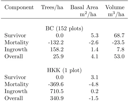
Table 1: Population net change estimates in British Columbia (BC) and Thai (HKK) data sets.
Component Trees/ha Basal Area Volume m2/ha m3/ha BC (152 plots)
Survivor 0.0 5.3 68.7
Mortality -132.2 -2.6 -23.5
Ingrowth 158.2 1.4 7.8
Overall 25.9 4.1 53.0
HKK (1 plot)
Survivor 0.0 3.1
Mortality -369.6 -4.8
Ingrowth 710.5 0.2
Overall 340.9 -1.5
2.1 BC Data: The BC data included 152 large stem-mapped, fixed-area permanent sample plots containing 20,807 trees. The plots were located throughout the BC interior (49◦–57◦N, 114◦–124◦W), covering a wide range of ecological and climatic conditions. The plot radii were either 12.65 m (20 plots), 16.06 m (106 plots), or 17.98 m (26 plots). Only the last growth period of each plot was kept for analysis. Growth periods were either 9 years (86 plots) or 10 years (66 plots). The DBH tagging limit was 9.1 cm. DBH at the beginning of the growth period ranged from 9.1 to 77.6 cm with a median of 14.3 cm.
2.2 HKK Data: The HKK data was obtained from a 1,000 m by 500 m (50 ha) permanent sample plot located at 15◦40N, 99◦10E containing 120,804 stem-mapped trees. The plot was measured three times (in 1994, 1999, and 2004), but only the last growth period (1999-2004) was used for analysis. The DBH tagging limit was 1.0 cm. DBH at the beginning of the growth period ranged from 1.0 to 402.5 cm with a median of 4.3 cm. Volume was not available for this data set.
2.3 Tree Classification: Trees were classified into four categories:
1. Live-and-in (L) trees were live, in the sample plot, and above the DBH tagging limit at the beginning (Time 1) and at the end (Time 2) of the growth period.
and above the DBH tagging limit at Time 1 and dead at Time 2.
3. Cut (C) trees were live, in the sample plot, and above the DBH tagging limit at Time 1 and re-moved before Time 2.
4. Recruitment trees (R) were not in the sample plot at Time 1 and live, in the sample plot, and above the DBH tagging limit at Time 2.
L trees are usually called survivor trees in the point sampling literature, which is a misnomer because some of the R trees are also trees that survived throughout the growth period. R trees are often split into more classes such as ingrowth, ongrowth, or nongrowth, but these sub-classes require knowing the DBH of the trees at Time 1.
3
Terminology
Beers (1962) identified five different definitions of “growth”. For this paper, the definition of interest was net change (or “net increase” in Beers’ terminology), de-fined as:
Δ2−1 = V2−V1 (3)
= ΔS+V2I−V1M−V1C (4) where Δ2−1 is the overall net change between Time 1
and Time 2;V1andV2are the stand-level live attributes
at Time 1 and Time 2, respectively; ΔS is the survivor change between Time 1 and Time 2; V2I is the stand-level attribute on ingrowth trees at Time 2; V1M is the stand-level attribute on Mortality trees at Time 1; and V1C is the stand-level attribute on Cut trees at Time 1. Survivor change is the change on trees that were live at Time 2 and above the DBH tagging limit at Time 1. In-growth trees are live and above the DBH tagging limit at Time 2 and below the DBH tagging limit at Time 1. Two common assumptions usually made when estimat-ing net change were also used for this study. Growth on Cut and Mortality trees between Time 1 and the time they were cut or died is ignored. Growth on trees that were below the DBH tagging limit at Time 1 and dead by Time 2 is also ignored.
4
Methods
The attributes investigated in this paper were number of trees/ha, basal area, and, for the BC data only, gross whole-stem volume/ha. Net change in each attribute was estimated using three methods:
1. Fixed-area plots;
2. Variable-radius plots and Flewelling’s method; and
3. Variable-radius plots and the cone implementation of Iles’ method.
The same sample trees are included with Flewelling’s and Iles’ methods, only the change estimators are differ-ent. The basal area factor (BAF) for the two methods based on variable-radius plots was selected individually for each permanent sample plot by taking the basal area of the full-size permanent sample plot at Time 1 divided by 6, rounded to the largest integer in order to have a variable plot with about 6 trees. BAF varied between 1 and 27 m2/hain the BC data with an average of 7 m2/ha. BAF was 6 m2/ha for all sample plots used in the HKK data.
The relative efficiency of different sampling designs or estimators can be expressed as the relative monetary cost to achieve a certain precision or relative precision for a certain monetary cost. The latter expression was em-ployed in this paper, following a similar study in which the sampling cost was fixed by selecting a plot radius and basal area factor (BAF) to yield a constant number of trees in each plot (Banyard 1976). The radius of the fixed-area plot was therefore reduced to match the cost of the two point sample-based methods so that their ef-ficiencies could be compared. The fixed-area plot radius (3.30 m for the BC data and 2.90 m for the HKK data) was iteratively computed to provide an average number of sample trees per measurement similar to the one ob-tained using variable-radius plots.
The attributes of interest at a point in time were com-puted using:
ˆ Vitk =
⎡ ⎣sit
j=1
yijt ⎤
⎦×phfkijt (5)
where ˆVitk is the estimator for the stand-level attribute of interest on plotiat timetusing methodk,yijtis the attribute of interest on tree j; phfkijt is the number of trees/ha each tree represents, and sit is the number of live trees in the sample plot.
The quantity phfkijtcan be estimated for each method using the following formulae:
phf FPijt = 10,000 πR2
i
(6)
phf ICijt = 3×
Dijt−dij Dijt
×BAFit
gijt (7)
phf Fijt = 1 gijt×
10,000 4−8ln(p)
×
DBHijt 100dij
2
It++
DBHijt p100Dijt
2
It−
(8)
fixed-area plot radius (m); gijt is the tree basal area (m2/ha);Dijtis the variable plot radius (m);dij is the distance (m) between the plot centre and the tree; pis the proportion of the variable plot radius where the tree-level BAF starts to decrease; DBH is the DBH (cm),It+ is an indicator variable that takes the following values:
It+ = 1 if 0.4Dijt< dij ≤Dijt (9) = 0 if 0≤dij≤0.4Dijt
andIt− is 1−It+.
The coefficient 3 in Equation (7) is the coefficient for a cone. The cone was used for this paper but other shapes having different coefficients are also possible. Flewelling (1981) was not specific about the relative distance where the BAF starts to decrease, other than recommending a value between 0.3 and 0.6. After examining his Figure 3, the value 0.4 (p= 0.4) was selected because it appeared to be an adequate choice for the range of growth rates shown in the figure (5%, 10%, 20%, and 40%).
Using Equations (4) and (5), Cut and Mortality change estimators can be defined as:
ˆ
VkMi1 = ⎡ ⎣m k i1 j=1
yij1
⎤
⎦×phfkij1 (10)
ˆ VkCi1 =
⎡ ⎣c k i1 j=1
yij1
⎤
⎦×phfkij1 (11)
where ˆV kMi1 and ˆVikC1 are the attribute estimators for the Cut and Mortality components, respectively, and mki1 and cki1 are the number of M or C trees, respectively. Since M and C trees behave similarly and there were no C trees in the BC data, both groups are reported as a single group under Mortality in the Results section.
Various estimators for the survivor and ingrowth com-ponents have been proposed in the past. An unbiased estimate of the sum of the survivor and ingrowth com-ponents can be defined as:
ˆ
ΔkSi +I =
lk i
j=1
yij2×phfkij2
−yij1×phfkij1
+ rk i j=1
yij2×phfkij2 (12)
where ˆΔkSi +I is the estimate of the sum of the survivor and ingrowth components, lki is the number of L trees, and rki is the number of R trees. Equation (12), how-ever, cannot easily be split into survivor and ingrowth components. While all L trees should be added within the survivor change component estimate, R trees should
be added to either the survivor or the ingrowth compo-nent estimate, but it is generally impossible to tell which trees belong to each component without additional in-formation.
If the DBH tagging limit was 0, or if DBH on border-line trees outside the plot were recorded at Time 1, or if R trees were cored, unbiased estimates of the survivor and ingrowth components would be possible:
ˆ ΔkSi =
lk i
j=1
yij2×phfkij2
−yij1×phfkij1
+ rk i j=1
yij2×phfkij2I +
ij (13)
ˆ VikI2 =
rk i
j=1
yij2×phfkij2(1−I +
ij) (14)
where ˆΔkSi and ˆVikI2 are unbiased estimators of the sur-vivor change (ΔS) and the ingrowth component (V2I) respectively using methodk, andIij+is an indicator vari-able (1 if DBH was above the tagging limit at Time 1, 0 otherwise). In most situations,Iij+ are unknown. One obvious biased option is to use a model to predict the unknown indicator variables. Bias is then introduced by the wrong predictions of the indicator variable. Grosen-baugh (1958) proposed an unbiased survivor component estimator:
ˆ ΔGSi =
lk i
j=1
(yij2−yij1)×phfkij1 (15)
where ˆΔGSi is Grosenbaugh’s net survivor change estima-tor, but this estimator can be larger then the unbiased estimate for the sum of the survivor and ingrowth com-ponents (Equation 12), leading to an inconsistency be-cause the estimate for ingrowth would then be negative to maintain additivity. Grosenbaugh, in a personal com-munication to Tim Gregoire, suggested rescaling ˆΔGSi to avoid negative ingrowth estimates (Gregoire 1993).
whose indicator variable is truly unknown, the estimated lower and upper bounds of the survivor component are:
ˆ Lki =
lk i
j=1
yij2×phfkij2
−yij1×phfkij1
+
bk i
j=1
yij2×phfkij2 (16)
ˆ
Uik = Lˆki +
wk i
j=1
yij2×phfkij2 (17)
where ˆLki and ˆUik are the estimated lower and upper bounds of the survivor component, respectively;bki is the number of B trees; andwki is the number of W trees. We then define the survivor net change component estimator as:
ˆ
ΔkSi =M IN( ˆUik, M AX( ˆLki,ΔˆGSi )) (18)
and the estimator for the ingrowth component as:
ˆ
VikI2 = ˆΔkS +I
i −ΔˆkSi (19)
For the HKK data set, 2,000 repetitions of a 50-point sample were simulated. Each sample followed a sys-tematic sampling design with a random start. The ini-tial point was randomly selected within the coordinates [(0 m, 100 m), (0 m, 100 m)] and subsequent plots were located with 100 m offset in both the x- and y-axes. The walkthrough method (Ducey et al. 2004) was applied to boundary overlap situations. The regularly shaped rect-angle used as boundary of the HKK data set meets the formal requirement for unbiasedness of the walkthrough method as stated by Ducey et al. (2004). The mean estimate of each sample was considered as a single ob-servation (sample size of 2,000).
Relative efficiency was defined as the ratio of the vari-ation of the plot estimate around the populvari-ation param-eter:
REk/l= 100× n
i=1(ˆyik−μ)
n
i=1(ˆyli−μ)
(20)
where REk/l is the relative efficiency of methodk with respect to methodl, ˆyki is either the plot-level change es-timate on ploti(BC data) or the mean plot-level change estimate in samplei (HKK data) using methodk;n is the number of observations (152 in the BC data and 2,000 in the HKK data); andμis the population param-eter. The population parameterμwas the true average change for the 152 plots in the BC data and the true change between 1999 (Time 1) and 2004 (Time 2) for the HKK data. RE greater than 100% indicates estima-torl is more efficient or the opposite if less than 100%.
Note that survivor change for trees/ha when using fixed-area plots is 0 by definition; relative efficiency based on that estimate is meaningless and doesn’t need to be cal-culated.
The bias of the change estimators was also computed using:
Biask = 1 n
n
i=1
ˆ
yki −μ (21)
where Biask is the bias due to estimatork.
All computations and simulations were completed within the statistical software R (R Development Core Team 2008).
5
Results
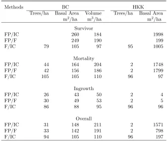
5.1 Relative Efficiency: Iles’ method was most ef-ficient for estimating overall net change in basal area and volume while the fixed-area plot estimator was most efficient for estimating overall net change in trees/ha (Table 2). Flewelling’s method was less efficient than Iles’ method for basal area and volume while it was slightly better for trees/ha. The difference in efficiency was larger in the HKK data than in the BC data.
The results for the net change components were simi-lar to the overall estimates, except that fixed-area plots were more efficient to estimate all ingrowth attributes. Ingrowth trees contribute little to basal area and are selected less frequently in point samples. This was par-ticularly the case in the HKK data where DBH ranged between 1 and 400 cm. More ingrowth trees would have been selected if two BAFs would have been used at each point. For instance, a BAF of 1 m2/ha for trees less
than 10 cm and the regular BAF for trees bigger than 10 cm could have been used. This strategy would have increased the probability of selection of trees less than 10 cm in point samples.
Table 2: Relative efficiency (%) of net change estimates in the BC and HKK data sets.
Methods BC HKK
Trees/ha Basal Area Volume Trees/ha Basal Area
m2/ha m3/ha m2/ha
Survivor
FP/IC 260 184 1998
FP/F 249 190 199
F/IC 79 105 97 95 1005
Mortality
FP/IC 44 164 204 2 1748
FP/F 42 156 186 2 1799
F/IC 105 105 110 96 97
Ingrowth
FP/IC 26 43 50 2 4
FP/F 30 49 53 2 5
F/IC 86 88 95 96 96
Overall
FP/IC 31 148 211 2 1571
FP/F 33 142 191 2 798
F/IC 94 105 110 96 197
bias when estimating survivor basal area. The observed bias associated with ingrowth and overall net change for trees/ha with Iles’ and Flewelling’s methods is more likely due to random variation because the proposed esti-mators are theoretically unbiased for trees/ha. Ingrowth trees were all less than 4 cm DBH in the HKK data. This translates into a maximum plot size of about 2 m2when
using a BAF of 6 m2/ha. Given the small plot areas
sur-rounding ingrowth trees, it appears that 100,000 plots (2,000 samples of 50 plots) were not close enough to in-finity to provide the theoretical answer, given the size of the population (50 ha).
6
Discussion
Furnival (1979) related his difficulties in convincing people that change can be estimated using point sam-ples. Husch et al. (1983, pp. 315–317) discussed com-mon concerns acom-mong foresters about estimating change using point samples. They dismissed most of the con-cerns but the compatibility issue remained (because they looked at only the Grosenbaugh (1958) estimator). Scott (1998) does not recommend point samples for permanent sample plots, mainly because of problems with estimat-ing the change components and that he did not con-sider the newer methods to estimate change in variable-radius plots.
As in many complex questions, the debate over fixed-area plots or point samples to estimate change should not be settled by a definite statistical answer. There are practical pros and cons to both plot layouts and it is im-portant to take these pros and cons into consideration when deciding what plot layout is best. Organizations wondering if they can re-measure existing point sam-ples to estimate change should be told it can be done, and that it is more efficient for volume and basal area. A network of existing point samples should not be dis-missed outright for change estimation because the past literature preferred fixed-area plots.
When only overall net change is needed (that is, no change component is required), variable-radius plots and Iles’ method should be considered. Iles’ method was more efficient at estimating overall change for basal area and volume than either fixed-area plots or Flewelling’s method and less efficient for trees/ha. Thus, whenever estimating change in basal area and volume are more important than change in trees/ha, variable-radius plots and Iles’ method would be an appropriate choice.
Table 3: Bias in net change estimates in British Columbia (BC) and Thai (HKK) data sets
Methods BC HKK
Trees/ha Basal Area Volume Trees/ha Basal Area
m2/ha m3/ha m2/ha
Fixed-Area
Survivor 0.0 0.5 7.5 0.0 0.0
Mortality -46.6 -2.7 -29.9 -2.7 0.2
Ingrowth -19.7 -0.2 -1.3 -4.1 0.0
Overall -66.3 -2.4 -23.6 -6.8 0.2
Iles
Survivor 0.0 0.3 4.8 0.0 0.0
Mortality -35.0 -1.9 -19.9 3.7 0.0
Ingrowth -8.8 -0.3 -1.6 18.8 0.0
Overall -43.8 -1.9 -16.6 22.4 0.0
Flewelling
Survivor 0.0 0.0 3.0 0.0 0.5
Mortality -43.8 -2.0 -21.2 2.1 0.0
Ingrowth -16.4 -0.1 -0.1 16.8 0.0
Overall -60.2 2.1 -18.2 18.9 0.5
and ingrowth change can be obtained with minimal ef-forts (Equations 13 and 14). There was, on average, only 1 and 0.5 R trees per plot in the BC and HKK data, respectively. If estimating ingrowth change is an important aspect of the permanent sample plot program, borderline trees outside the plot should be measured for distance and DBH, and eliminated from the compilation by the compilation software. The only measurement re-quired on these borderline trees outside the plot is DBH to be able to determine if they were above or below the tagging limit at the previous measurement. Modifying the compilation software to flag these trees should not be onerous.
A constrained version of the Grosenbaugh (1958) sur-vivor estimator can be used to estimate sursur-vivor change. The ingrowth estimator derived from Equation (12) and the constrained Grosenbaugh estimator (Equation 18) is always positive. The potential for bias can be drasti-cally reduced by reducing the number of W trees (trees where the status above or below the DBH tagging limit is truly unknown). A careful review of the R trees and available information (site index, relative DBH growth on L trees, etc.) should help reduce the number of W trees. In the two data sets used for this paper, W trees were present on only 24% and 3% of the plots in the BC and HKK data sets, respectively. The bias will never be eliminated using this estimator, but it could be made practically insignificant.
Fixed-area plots were more efficient for estimating change in all ingrowth attributes and trees/ha, while Iles’ method was more efficient for estimating change in volume and basal area for the survivor and mortal-ity components. Variable-radius plots are inefficient for quantifying ingrowth of small trees simply because those trees are sampled at a lower frequency than survivor trees. Whenever ingrowth is an important attribute re-quiring a change estimate, fixed-area plots are the most efficient plot layout. It is also possible to use both fixed-area plots for trees under a certain size and variable-radius plots for larger trees. Using multiple plot layouts centered at one sampling point is an efficient sampling strategy when sampling for different resources. The same idea can be applied when estimating change for ingrowth and survivor trees.
for establishing a network of permanent sample plots for research purposes.
Finally, the importance of recording in the field the distance between the sampling point and the trees in variable-radius plots must be emphasized. Range find-ers and lasfind-ers now make this task very simple. Stem-mapping should become a standard inventory practice to facilitate future use of variable-radius plots. The ex-tra time in the field to record the information is minimal, changes to the database to store the information are sim-ple, and modifications to the data compilation software are straightforward and will allow the software to com-pute change. Organizations with stem-mapped perma-nent sample plots can easily test Iles’ method over multi-ple measurements and various forest types and compare the results to their traditional estimators.
7
Conclusions
Foresters have refrained from using variable-radius plots for estimating change over concerns about the sta-tistical efficiency and compatibility of change estimates. The new change estimator proposed by Iles and Carter (2007) was shown to be more efficient than the fixed-area plot estimator for basal fixed-area and volume for overall net change. Compatibility and time additivity are no longer an issue undermining the credibility of change estimates based on point samples. The perceived com-plexity due to the expanding inclusion zone is no longer a problem. Iles’ method can be retro-fitted on existing stem-mapped fixed-area permanent sample plots (after checking for possible large trees outside the plots) and its accuracy compared to traditional change estimates. Change component estimators for point samples exist and can be unbiased under certain unrestrictive condi-tions (tagging limit is 0, or DBH of borderline trees is recorded, or recruitment trees are cored). Point-to-tree distance is now a simple measurement that should be recorded in all forest management inventories. Finally, forestry students should be taught that point samples can be used efficiently to estimate change.
Acknowledgments
The final version of the paper benefited from the com-ments of Greg ONeill, Kim Iles, and two anonymous reviewers. Jon Vivian provided the BC data, while Sarayudh Bunyavejchewin, Peter Ashton, and Stuart Davies provided the HKK data. The establishment and ongoing conduct of research at the HKK plot is sup-ported by the Center for Tropical Forest Science, Smith-sonian Institution, and through grants from the United States National Science Foundation.
References
Afanasiev, M., 1958. Some results of the use of the Bit-terlich method of cruising in an even-aged stand of longleaf pine. J. For. 56:341–343.
Banyard, S., 1976. A comparison between point sam-pling and plot samsam-pling in tropical rain forest based on a concept of the equivalent relascope plot size. Com-monwealth For. Rev. 54:312–320.
Beers, T., 1962. Components of forest growth. J. For. 60:245–248.
Beers, T., and C. Miller, 1964. Point sampling: research results, theory and application. Agric. Exp. Stn. Res. Bull. 786, Purdue Univ., West Lafayette, IN.
Bell, J., and L. Alexander, 1957. Application of the variable plot method of sampling forest stands. Res. Note 30, Oregon Board of Forestry, Salem, OR.
Bitterlich, W., 1947. Die winkelzahlmessung. All. Forst-u. Hozwirtsch. Ztg. 58:94–96.
Bitterlich, W., 1984. The relascope idea: relative mea-surements in forestry. Commonwealth Agricultural Bureaux, Slough, UK.
Bruce, D., 1961. Prism cruising in the western United States and volume tables for use therewith. Mason, Bruce, & Girard Inc. Portland, OR.
Carter, D., 2007. An assessment of variable radius plot sampling techniques for measuring change over time: a simulation study. Master’s thesis, University of British Columbia.
Ducey, M., J. Gove, and H. Valentine, 2004. A walk-through solution to the boundary overlap problem. For. Sci. 50:427–435.
Ericksson, M., 1995. Compatible and time-additive change component estimators for horizontal point-sampled data. For. Sci. 41:796–822.
Flewelling, J., 1981. Compatible estimates of basal area and basal area growth from remeasured point samples. For. Sci. 27:191–203.
Furnival, G., 1979. Forest sampling — past performance and future expectations. In Forest Resource Invento-ries Workshop Proceedings. Vol.1, Frayer, W., ed., pp. 320–326. Colorado State University, Fort Collins, CO.
Gregoire, T., 1993. Estimation of forest growth from successive surveys. For. Ecol. Manag. 56:267–278.
Grosenbaugh, L., 1958. Point-sampling and line-sampling: Probability theory, geometric implications, synthesis. Occ. Paper 160, USDA For. Serv. South. For. Exp. Stn.
Hradetzky, J., 1995. Concerning the precision of growth estimation using permanent horizontal point samples. For. Ecol. Manag. 71:203–210.
Husch, B., C. Miller, and T. Beers, 1983. Forest Men-suration. John Wiley & Sons, New York, NY.
Iles, K., 1981. Permanent “variable” plots for forest growth. Presentation to the Western Mensurationists Conference. Sun Valley, ID.
Iles, K., and D. Carter, 2007. “Distance-variable” esti-mators for sampling and change measurement. Can. J. For. Res. 37:1669–1674.
Martin, G., 1982. A method for estimating ingrowth on permanent horizontal sample points. For. Sci. 28:110– 114.
R Development Core Team, 2008. R: A Language and Environment for Statistical Computing. R
Founda-tion for Statistical Computing, Vienna, Austria. URL http://www.R-project.org. ISBN 3-900051-07-0.
Roesch, F., E. Green, and C. Scott, 1989. New com-patible estimators for survivor growth and ingrowth from remeasured horizontal point samples. For. Sci. 35:281–293.
Scott, C., 1998. Sampling methods for estimating change in forest resources. Ecol. Appl. 8:228–233.
Scott, C., and J. Alegria, 1990. Fixed versus variable radius plots for change estimation. In State-of-the-art methodology of forestry inventory: a symposium proceedings, LaBau, V., and T. Cunia, eds., pp. 126– 132. USDA Forest Service, Pacific Northwest Research Station. PNW-GTR-263.
Spurr, S., 1952. Forest Inventory. Ronald Press Co., New York, NY.