Forestry & Natural-Resource Sciences Last Correction: Sep. 30, 2016
SPATIAL INTERPOLATION OF ABOVE-GROUND BIOMASS IN
LABANAN CONCESSION FOREST IN EAST KALIMANTAN,
INDONESIA
Taek Joo Kim
1, Bronson P. Bullock
2, Arief Wijaya
31
Department of Forestry and Environmental Resources, North Carolina State University, Raleigh, NC, USA 2
Warnell School of Forestry and Natural Resources, University of Georgia, Athens, GA, USA 3Th¨unen Institute of International Forestry and Forest Economics, Hamburg, Germany
Abstract.This study applied a geostatistical approach to quantify above-ground biomass (AGB) of
the Labanan Concession Forest in East Kalimantan, Indonesia. Forest inventory data collected via line-plot sampling were converted to AGB, and two approaches of estimating the spatial distributions of biomass, the global and stratified approaches, were compared. The global approach does not take local varying structures into account, whereas the stratified approach accounts for the heterogeneity of land cover types. Thus, AGBs estimated from each land cover type were pooled for the stratified approach. Ordinary kriging was performed to predict AGB at unsampled locations. The total estimates of AGB and root mean squared cross-validation errors (RMSCVE) for the global and stratified methods were 13,512,392.2 tons (161.92 ton/ha) and 13,607,205.5 tons (163.05 ton/ha), respectively, for AGB (0.7% difference) and 81.0 ton/ha and 81.2 ton/ha, respectively, for RMSCVE. Considering the different environmental conditions for each land cover type, the stratified method was expected to better capture the spatial structure particular to each land cover type, leading to more accurate es-timates of AGB. However, the results suggest the degree of accuracy for the two methods was nearly similar.
Keywords: Spatial dependency, Line-plot sampling, Landscape heterogeneity, Ordinary kriging.
1
Introduction
Quantification of forest biomass is essential to assess forest growth and productivity. Quantification of for-est biomass is also important to for-estimate carbon stored in a forest because carbon comprises about half of the dry biomass (Brown 1997). Due to the significant role of forests involved in the global carbon cycle (Pan et al. 2011), precise measurements of forest biomass is cur-rently one of the most critical issues in the research of global climate change and carbon flux and sequestration in forests (Tanase et al. 2014), and quantifying forest biomass has gained a fair amount of interest over the past few decades (Usuga et al. 2010). Since field data of below-ground biomass cannot be collected easily, above-ground biomass (AGB) has usually been the only part of the carbon entity that has been estimated (Lu 2006).
So far, the estimation of AGB has been derived from techniques based on field measurements, remote sens-ing, and Geographic Information System (GIS) analysis
(Lu 2006; Wijaya et al. 2010a). Field measurements are obtained directly by felling trees and cutting them into sections, and then the parts are oven dried and weighed to derive estimate of AGB (Brown 1997). This method is known to be the most accurate way for estimating AGB by far (Djomo et al. 2010). Indirect tree measure-ments of AGB such as stem diameter or total height are often correlated to develop allometric equations for AGB estimation (Pearson et al. 2007; Basuki et al. 2009; Djomo et al. 2010; Blujdea et al. 2012; Rutishauser et al. 2013) that can then be used in subsequent estima-tions. In estimating AGB over a large region, a remote sensing method is useful, and is especially effective in assessing AGB in inaccessible areas where data collection is difficult (Lu 2006). Airborne small-footprint Light Detection and Ranging (LiDAR) is currently being eval-uated as the most promising tool for estimating spatial distributions of AGB over large areas (Laurin et al. 2014). Environmental measurements such as tree height,
malized Difference Vegetation Index (NDVI), and Leaf Area Index (LAI) obtained from remote sensing data are correlated with ground measurements of AGB since direct measurements of AGB are not available through remote sensing techniques (Saatchi et al. 2007; Basuki et al. 2009; Tsui et al. 2013). A GIS approach to estimate AGB is based on superimposing maps of supplementary information such as elevation, slope, soil, precipitation, and land cover into the GIS software (Lu 2006; Wijaya et al. 2010a) and then using this information to aid in AGB estimation.
In this work, a geostatistical approach was applied to estimate the spatial distribution of AGB over a forest region. Unlike the approaches aforementioned, geostatis-tics treats the observed data in the context of their locations by looking at the relationship in terms of dis-tance between each point. Geostatistics takes stochastic assumptions on the observed dataset. The stochastic approach has the advantage of estimating the errors for the prediction. Spatial variation is assessed through var-iograms. Variograms model spatial dependency among the data as a function of distance. Based on the model of the variogram, predictions are made. The prediction is referred to as kriging in geostatistics (Ripley 1981; Webster and Oliver 2007).
Geostatistical methods have been widely used in the research of forestry to analyze spatial distribution and mapping of AGB over large areas. Two different ap-proaches to derive spatial structures of AGB were applied according to the availability of secondary information, of which a lot of work using secondary information can be found in remote sensing applications. With available ground based AGB data, the deterministic part of AGB was modeled using remote sensing data (i.e., LiDAR, spec-tral bands, vegetation indices, satellite images, etc.) with which environmental variables are often combined (i.e., soils, vegetation type, elevation, etc.). After removing the deterministic part from AGB, the spatial structure of the residuals is assessed for kriging. Different kriging techniques have been applied including ordinary kriging regression kriging, co-kriging, and universal kriging (De Jong et al. 2003; Freeman and Moisen 2007; Sales et al. 2007; Castillo-Santiago et al. 2013; Lamsal et al. 2012; Tsui et al. 2013; Zhang et al. 2014; Galeana-Piza˜na et al. 2014). On the contrary, in cases without secondary information, some research directly explored spatially varying structures of AGB. Kriging estimates of AGB were derived from the model of spatial dependency of AGB (Hero et al. 2013).
The objective of this study was to explore the struc-ture of spatial continuity of AGB collected by line-plot sampling and estimate the total biomass in an Indone-sian forest applying a geostatistical approach. Line-plot sampling is known to efficiently reflect varying structures
of land cover types (Tiryana 2005), which makes it useful for capturing spatial structures of collected data. Two estimates of AGB, global and pooled, were assessed. The global estimate uses the entire dataset for prediction without considering the varying local structures (land cover types). On the other hand, the pooled estimate accounts for the different local structures and the AGB assessment of each separate stratum is added to calculate the total AGB. Finally, a cross validation was performed to check the accuracy of the kriging estimates.
2
Ordinary Kriging
Let us define Z(s) as a realized value from a spa-tial stochastic processZ(), wheres is the location of variableZ(s) in domainD of R2. The variation and con-tinuity of realized single values from a spatial stochastic processZ(s) is characterized through an experimental variogram. An experimental variogram ˆΥ(h) estimates spatial dependence and is quantified by the average dif-ference between the pairs of sampled values according to their lag distance.
ˆ
Υ (Hk) = 1 2nk
nk
X
i=1
(Z(si+h)−Z(si))2
where:
nk is the numbers of pairs of samples separated apart by the length of vectorh(h∈Hk); and
si is the location where variableZ(si) is sampled.
A typical plot of experimental variogram has an in-creasing trend and reaches an asymptote as the length of vectorhincreases (Wackernagel 2003). The maximum value of the asymptote is called the sill and the range is the lag distance at which sill is reached. The discontinu-ity behavior at microscale near the origin, whereh= 0, is called the nugget effect. The discontinuity indicates dras-tic changes of sample values at very short lag distances. Although the estimated value of experimental variogram must be 0 ath= 0, dissimilarity of sampled values at very short lag distances results in discontinuity ath= 0, in other words, non-zero positive value ath= 0 (Isaaks and Srivastava 1989). After the experimental variogram is estimated, the theoretical variogram is fitted. The theoretical variogram ensures that the covariance of the kriged estimate, which is a linear weighted sum of sample values, is non-negative (Schabenberger and Pierce 2002; Wackernagel 2003).
(Webster and Oliver 2007). Ordinary kriging is applied when the spatial processes are second-order or intrinsic stationary (Schabenberger and Pierce 2002). If the mean E[Z(s)] =uis constant and the covariance function is dependent only on the distance separated byhbetween the two spatial points,C(h) = E[(Z(s) –u)(Z(s+h) – u)], the spatial stochastic process is said to be second-order stationary (Kitanidis 1997; Schabenberger and Pierce 2002; Montes and Ledo 2010), whereas the intrin-sic stationarity is defined by the mean and variances of the differences ofZ(s) –Z(s+h).
In kriging, an unknown value of Z0=Z(s0) is esti-mated by weighted linear average of observations from other measured locationss1, s2, . . . , sn, whereλis are kriging weights such that
ˆ Z0= n X i=1 λiZ(si)
and in ordinary kriging, λis should satisfy the
follow-ing two conditions: (1) unbiasedness where n
P
i=1 λi= 1
so that the expectation of estimation error is zero and unbiasedness is guaranteed, and (2) minimum variance of the estimation error (Isaaks and Srivastava 1989; Ki-tanidis 1997).
3
Materials and Methods
3.1 Study area This study analyzed the data col-lected from Labanan concession forest, the district of Be-rau East Kalimantan Indonesia (Figure 1). The Labanan concession forest is located near the equator within the geographic coordinates of 1◦45’ to 2◦10’ N and 116◦55’ to 117◦20’ E. The size is approximately 83,000 ha. The Labanan concession forest is situated in the interior land of coastal swamps and has diverse geographical and to-pographical features comprising of plains, slopes, steeps, and complex landforms with elevations ranging from 50 to 650 m. The landscape is characterized by aggregates of high hills and mountains sporadically spread across fluctuating plain surfaces. The forest type of the La-banan concession forest is a mixed lowland dipterocarp forest and categorized as a tropical moist forest. The temperature ranges from 23-33◦C with 26◦C on average and the mean annual rainfall is 2,000 mm. The Labanan concession forest is operated by PT Inhutani I, a state owned company, and selective logging practices have been prevalent in the area since the 1970’s (Wijaya et al. 2010a; Wijaya et al. 2010b)
3.2 Data and sampling plot descriptions Diam-eter at Breast Height (DBH) data of dipterocarp species collected from 1,460 sampling plots distributed across 16
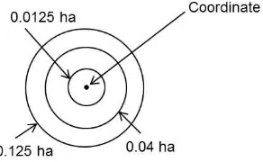
line-plots during April 1997 and January 1998 were used. A total of 13,050 trees with DBH ranging from 10 to 210 cm were measured (Wijaya et al. 2010a). Line-plot sampling was conducted in the direction of northwest 135◦ (Tiryana 2005). In each of the sixteen line-plots, plots were established at a distance between 60 m and 225 m with most of the plots about 100 m apart. The perpendicular distances between line-plots were approxi-mately 2,000 m to 6,000 m apart averaging 5,000 m. The plot is a nested design and comprised of three levels of circular sub-plots, 0.125 ha for DBH>50 cm (radius of 19.95 m), 0.04 ha for DBH 20-49 cm (radius of 11.28 m), and 0.0125 ha for DBH 10-19 cm (radius of 6.31 m) with coordinates collected in the center of each plot (Figure 2). In addition to the DBH data, the land cover type of each plot was assessed and recorded. In total, eight land cover types were associated with the line-plots. A map of the concession area classified by land cover type is also available in a shape file format. There are four more land cover types recorded in addition to the eight land cover types associated with the line-plots, thus totaling 12 land cover types available in a shape file format. The land cover type data were obtained from Landsat Thematic-Mapper (TM) multi-spectral satellite images. The images were geometrically corrected and rectified with a 1:25,000 hydrology map to match the UTM 50 grid. The raw image was first enhanced with a contrast stretching, and then the enhanced image was classified into different land cover types based on visual interpretations, from which both textural and spectral features could be evaluated. For the verification, field vis-its were conducted, based on which the classification was later updated. The classified information of land cover types is described in Table 1 (Berau Forest Management Project 2001).
3.3 Derivation of AGB data An allometric equa-tion based on DBH (cm) was used to calculate AGB. The equation was developed by harvesting and destruc-tively sampling a total of 40 trees from 28 genera with DBH varying from 6 to 68.9 cm from tropical lowland dipterocarp forests (Samalca 2007; Wijaya et al. 2010a).
AGB= exp(−1.2495 + 2.3109×ln(DBH))
Figure 1: Map of Labanan concession forest in East Kalimantan, Indonesia by land cover and line-plots. The letters are land cover type abbreviations, and they are described in Table 1.
Figure 2: Nested plot design used for sampling at each plot.
3.4 Global vs. stratified method Two different approaches were applied to estimate the spatial distribu-tion of AGB: global and stratified. The global method assumes a single correlation structure throughout the whole domain and uses all line-plot data, whereas the stratified method separately treats the data according to their land cover type. The stratified method assumes that each stratified domain will have a spatial process
particular to each stratum. The total AGB for the strati-fied method should be pooled based on the AGB estimate for each land cover type. However, the basic approaches for modeling the variograms and kriging are the same for both methods following the usual steps for geostatistical approach.
3.4.1 Variogram modeling Experimental variograms were only assessed in the directional angle of 135◦since
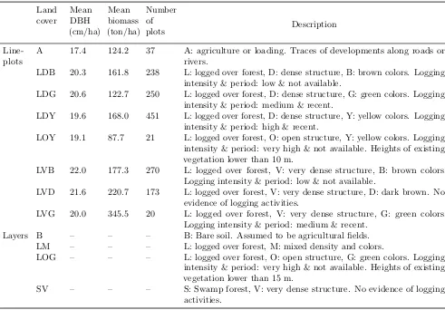
Table 1: Measurements and descriptions for each land cover type. As noted, the last four land covers (B, LM, LOG, SV) are only available as shape file layers and not used in the analysis (Berau Forest Management Project 2001).
Land cover
Mean DBH (cm/ha)
Mean biomass (ton/ha)
Number of
plots Description
Line-plots
A 17.4 124.2 37 A: agriculture or loading. Traces of developments along roads or rivers.
LDB 20.3 161.8 238 L: logged over forest, D: dense structure, B: brown colors. Logging intensity & period: low & not available.
LDG 20.6 122.7 250 L: logged over forest, D: dense structure, G: green colors. Logging intensity & period: medium & recent.
LDY 19.6 168.0 451 L: logged over forest, D: dense structure, Y: yellow colors. Logging intensity & period: high & recent.
LOY 19.1 87.7 21 L: logged over forest, O: open structure, Y: yellow colors. Logging intensity & period: very high & not available. Heights of existing vegetation lower than 10 m.
LVB 22.0 177.3 270 L: logged over forest, V: very dense structure, B: brown colors. Logging intensity & period: low & not available.
LVD 21.6 220.7 173 L: logged over forest, V: very dense structure, D: dark brown. No evidence of logging activities.
LVG 20.0 345.5 20 L: logged over forest, V: very dense structure, G: green colors. Logging intensity & period: medium & recent.
Layers B – – – B: Bare soil. Assumed to be agricultural fields. LM – – – L: logged over forest, M: mixed density and colors.
LOG – – – L: logged over forest, O: open structure, G: green colors. Logging intensity & period: very high & not available. Heights of existing vegetation lower than 15 m.
SV – – – S: Swamp forest, V: very dense structure. No evidence of logging activities.
Note: Brown colors (slightly logged), dark brown colors (very dense forest structure), green colors (moderately logged), and yellow colors (very heavily logged) reflect variation in the dominant colors besides red pixels (vegetation) from the satellite imagery. The satellite image was enhanced by contrast stretching and the colors are closely related to the stretching.
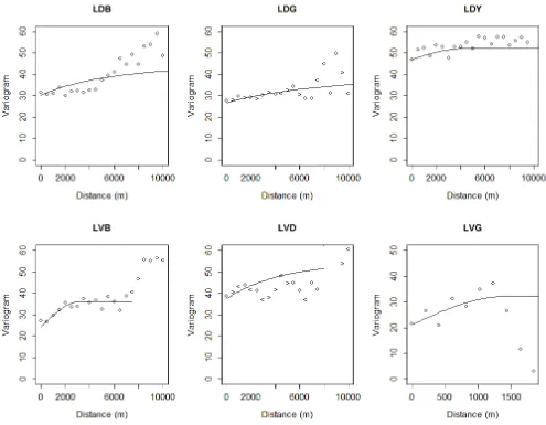
anisotropy was not possible due to the fact that line-plots were aligned in one direction. Webster and Oliver (2007) suggest three sampling directions at minimum to detect anisotropy in line-plot sampling. The lag interval was set to 1,000 m for the global method and 500 m for the stratified method except for LVG which was set to 205 m and the maximum lag distance of LVG was also confined to 3,000 m since the area for estimation was smaller than the others. Lag intervals were determined as such to estimate long range predictions although the plots were systematically collected at the average distance of 100 m along line-plots. Otherwise, predictions may not be continuous over long ranges if short range correlation is estimated (Goovaerts 1997). In our case, predictions between line-plot distances, which are approximately 5,000 m apart, may not show smooth transitions. The theoretical variogram model was fitted using weighted least squares, maximum likelihood (ML), and restricted
maximum likelihood (REML). The best fitted variogram model was selected depending on how well range pa-rameters and trends after reaching an asymptote were realistically fitted considering the size of the study area and each land cover type among the three methods.
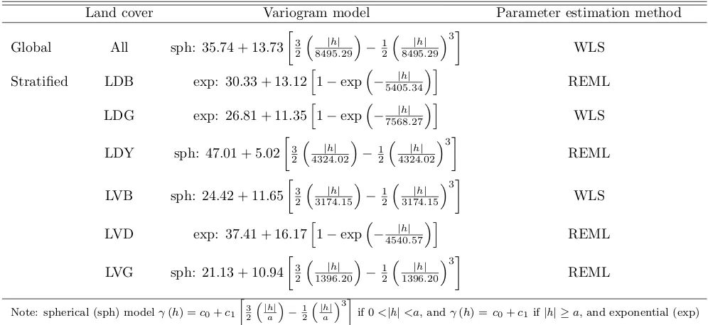
Table 2: Theoretical variogram models by global and stratified methods (WLS: weighted least squares, REML: restricted maximum likelihood).
Land cover Variogram model Parameter estimation method
Global All sph: 35.74 + 13.73
3 2
|h|
8495.29
−1 2
|h|
8495.29
3
WLS
Stratified LDB exp: 30.33 + 13.12h1−exp−5405.34|h| i REML LDG exp: 26.81 + 11.35h1−exp−7568.27|h| i WLS LDY sph: 47.01 + 5.02
3 2
|h|
4324.02
−1 2
|h|
4324.02
3
REML
LVB sph: 24.42 + 11.65
3 2
|h|
3174.15
−1 2
|h|
3174.15
3
WLS
LVD exp: 37.41 + 16.17h1−exp−4540.57|h| i REML LVG sph: 21.13 + 10.94
3 2
|h|
1396.20
−1 2
|h|
1396.20
3
REML
Note: spherical (sph) modelγ(h) =c0+c1 3 2 |h| a −1 2 |h| a 3
if 0<|h|<a, andγ(h) =c0+c1 if|h| ≥a, and exponential (exp)
modelγ(h) =c0+c1 h
1−exp
−|h|
a
i
, wherec0: nugget,c1: sill,a: range, andh: lag.
multi-layered structures perpendicular to each line-plot if the number of neighbors is limited, since the distances between each plot, which are much smaller than the dis-tances between each line-plot strongly affects predictions. After kriging, kriging estimates of AGB were clipped to the boundary of the concession area for the global method and each land cover type for the stratified method. The associated standard deviations of kriging estimates are also presented.
3.5 Validation The two kriging estimates were com-pared by applying “leaving-one-out cross-validation” (Ribeiro and Diggle 2001), a validation method that deletes one sample data in sequence from the dataset and then mak-ing a prediction at the removed location with n – 1 remaining sample data. This procedure is conducted until every sample data location is estimated (Wacker-nagel 2003). We applied the root mean squared cross-validation errors (RMSCVE) approach for the perfor-mance comparison of the two kriging estimates
RMSCVE = v u u t n P i=1 h
Z(si)−Z(si)ˆ i 2 n
where ˆZ(si) is the estimated value at locationsi. The variogram analysis and kriging was conducted using the geoR package (Ribeiro and Diggle 2001) of the statistical software R (R Core Team 2014). ArcMap 10.2
was used for clipping kriging estimates exported from R and map production (ESRI 2013).
4
Results and Discussion
increas-Table 3: Estimated total biomass from kriging.
Kriging estimates of biomass (ton)
Land cover Global Stratified Difference: Stratified – Global (ton) Percentage difference (%)
LDB 2,807,097.3 2,889,151.5 82,054.2 2.9
LDG 1,744,102.7 1,589,901.3 -154,201.4 9.3
LDY 3,109,625.6 3,137,919.9 28,294.3 0.9
LVB 3,283,258.6 3,302,659.1 19,400.5 0.6
LVD 1,563,045.2 1,679,084.0 116,038.8 7.2
LVG 22,804.7 26,031.6 3,226.9 13.2
Others 982,458.1 982,458.1 – –
Total 13,512,392.2 13,607,205.5 94,813.3 0.7
Note:Others land cover class includes land cover A, B, LM, LOG, LOY, and SV.
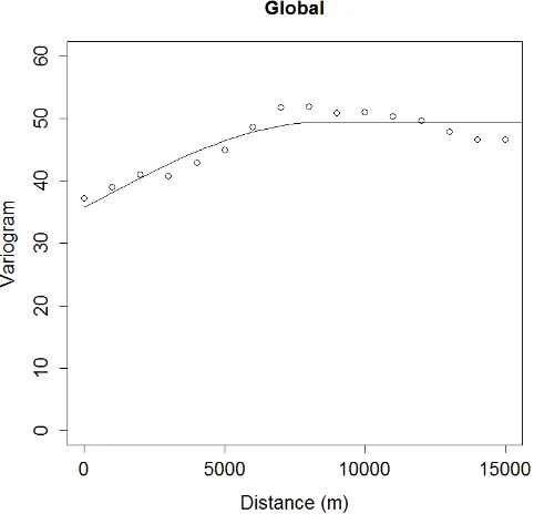
ing trends at short lag distances. Graphs of global and stratified variogram models are presented in Figure 3 and 4.
Figure 3: Global variogram using all land cover types combined. Experimental and theoretical variograms are depicted as open dots and a full line, respectively.
One thing to note is that the variograms for line-plot data of land cover A and LOY were not analyzed. Land cover A did not have an appropriate experimental variogram model for a theoretical variogram model, and in land cover LOY, the shape of map of the land cover was not suitable for the line-plot data to make predictions
within the land cover (refer to Figure 1). In other words, the line-plot data of LOY was not properly arranged within the land cover for kriging. How land cover A and LOY were treated is explained in detail in the following section.
4.2 Kriging estimates and estimation variances
The total AGB kriging estimates of the global and strat-ified methods were 13,512,392.2 (161.92 ton/ha) and 13,607,205.5 tons (163.05 ton/ha), respectively. The stratified method had a larger estimate, of which the dif-ference between the two estimates is 94,813.3 tons (0.7% difference in the estimates). Stratified method had larger estimates for each land cover type except for the land cover LDG. Lower kriging estimates of land cover LDG may be the result of the LDG data itself. The smaller mean value of AGB for land cover LDG suggests that the actual biomass measurements are lower compared to the other land covers. The lower global estimate is probably due to the number of weights assigned for krig-ing each grid (recall that global neighborhood is applied and the number of neighbors is 1,460). The weights of nearest line-plot data to each target grid for kriging may have been smoothed out because of the number of neighbors. The nearest weights account for the greatest portion of the total weight (Webster and Oliver 2007). As mentioned previously, land cover A and LOY were not individually analyzed. Land cover A and LOY were included together within the categoryothers, of which line-plot data of land cover were not available but only the layers of shape files (B, LM, LOG, SV). The estimate of categoryothers is subtracted value of the other land covers from the total estimate of global method (Table 3).
Figure 4: Stratified variograms. Experimental and theoretical variograms are depicted as open dots and full lines, respectively. Note the different maximum lag distances fitted to LVB (7,500 m), LVD (8,000 m), and LVG (3,000 m).
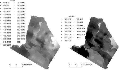
ranged from 81.3 ton/ha (LVG) to 342.1 ton/ha (LVD) for the global method, and from 80.8 ton/ha (LDG) to 360.3 ton/ha (LVG) for the stratified method. The spatial distribution of AGB kriging estimates were largely affected by the arrangement of the line-plots, as indicated by Figures 5 and 6. Although there were indications of logging activities along the roads and near villages within the site, where low densities of AGB can be observed, incorporating specific features of the landscape into the kriging estimates of AGB was not possible due to the lack of data. The standard deviations of the estimate are small close to the line-plots and become larger as the distance increases away from the line-plots. It can be observed that standard deviations are also large in regions where kriging estimates are large. This is due to
the transformation of the original data using a square root in the analysis, whereλ= 0.5 for Box-Cox transformation in our case (Diggle and Ribeiro 2007). Note that kriging estimates and standard deviation are discontinuous by each land cover type in the map of the stratified method.
cap-Figure 5: Maps of kriging estimates of AGB (left) and associated standard deviation (right) of the global method.
turing spatial structures particular to each land cover type, would exhibit more accurate result than the global method. However, the accuracy of both methods was actually largely affected by high nuggets in the predic-tion, as suggested by associated standard deviations of predictions.
5
Conclusions
This study estimated above-ground biomass (AGB) of Labanan concession forest in Indonesian using two differ-ent kriging approaches: a global method and a stratified method. The stratified method had a larger estimate of total biomass over the area by 95,000 tons (0.7% dif-ference). By evaluating the accuracy of AGB estimates by cross-validation, it was difficult to conclude that the one method has an advantage over the other method. Standard deviations associated with kriging estimates were also relatively high due to high nugget effects for both methods. Nugget effects may be reduced by devel-oping a more precise model of AGB so that measurement error can be reduced, or increasing sampling intensity by establishing more plots between each sampling line to better estimate spatial structures.
For a better assessment of accuracy in the estimates, a more realistic approach would be comparing estimates obtained from different methods such as remote sens-ing, or more extensive collection of data from ground measurements. Depending on the validation criteria for comparing true and estimated values, non-geostatistical methods could yield better estimates of AGB. For exam-ple, Freeman and Moisen (2007) applied a geostatistical approach to improve the initial estimates of AGB assessed from nonparametric methods with kriging residuals but found no noticeable improvement in minimizing mean squared error (MSE). Zhang et al. (2014) showed that a non-geostatistical multiple regression model (R2= 0.60) had better estimates of AGB than the kriging method (R2= 0.29). The suggested nonparametric and multiple regression models in the two examples were estimated using remote sensing data and environmental variables. Therefore, it is advisable to apply both geostatistical and non-geostatistical methods especially when AGB can be modeled by secondary information.
Finally, the geostatistical approach may be one of the most useful techniques in the aspect of data requirements and cost efficiency to estimate AGB over a large region. Required information are ground based AGB estimates and their associated locational data. To apply this geo-statistical approach, it is important to check if the spatial process of the region of interest is stationary and has a proper model of spatial dependency for prediction.
Acknowledgement
The authors would like to thank PT Inhutani I La-banan Forest Management for collecting and providing the data. The authors would also like to thank the two anonymous reviewers for their helpful comments that greatly contributed to improving the manuscript.
References
Basuki, T.M., P.E. van Laake, A.K. Skidmore, and Y.A. Hussin. 2009. Allometric equations for estimating the above-ground biomass in tropical lowlandDipterocarp forests. Forest Ecology and Management. 257(8): 1684– 1694.
Berau Forest Management Project. 2001. Mapping veg-etation and forest types using Landsat TM in the Labanan concession of PT Inhutani I. Berau Forest Management Project. 16 p.
Berthouex, P.M., and L.C. Brown. 2002. Statistics for en-vironmental engineers. 2ndedition. Boca Raton, Lewis Publishers. 489 p.
Blujdea, V.N.B., R. Pilli, I. Dutca, L. Ciuvat, and I.V. Abrudan. 2012. Allometric biomass equations for young broadleaved trees in plantations in Romania. Forest Ecology and Management. 264: 172–184.
Brown, S. 1997. Estimating biomass and biomass change of tropical forests: A primer. FAO Forestry Paper 134. UNFAO, Rome, Italy. 55 p.
Castillo-Santiago, M. ´A., A. Ghilardi, K. Oyama, J.L. Hern´andez-Stefanoni, I. Torres, A. Flamenco-Sandoval, A. Fern´andez, and J. Mas. 2013. Estimating the spatial distribution of woody biomass suitable for charcoal making from remote sensing and geostatistics in central Mexico. Energy for Sustainable Development. 17(2): 177–188.
De Jong, S.M., E.J. Pebesma, and B. Lacaze. 2003. Above-ground biomass assessment of Mediterranean forests using airborne imaging spectrometry: The DAIS Peyne experiment. International Journal of Re-mote Sensing. 24(7): 1505–1520.
Diggle, P.J., and P.J. Ribeiro. 2007. Model-based geo-statistics. New York, NY, Springer. 228 p.
Djomo, A.N., A. Ibrahima, J. Saborowski, and G. Graven-horst. 2010. Allometric equations for biomass estima-tions in Cameroon and pan moist tropical equaestima-tions including biomass data from Africa. Forest Ecology and Management. 260(10): 1873–1885.
Fortin, M.J., and M.R.T. Dale. 2005. Spatial analysis: A guide for ecologists. Cambridge, UK, Cambridge University Press. 365 p.
Freeman, E.A., and G.G. Moisen. 2007. Evaluating krig-ing as a tool to improve moderate resolution maps of forest biomass. Environmental Monitoring and Assess-ment. 128(1-3): 395–410.
Galeana-Piza˜na, J.M., A. L´opez-Caloca, P. L´opez-Quiroz, J.L. Silv´an-C´ardenas, and S. Couturier. 2014. Mod-eling the spatial distribution of above-ground carbon in Mexican coniferous forests using remote sensing and a geostatistical approach. International Journal of Applied Earth Observation and Geoinformation. 30: 179–189.
Goovaerts, P. 1997. Geostatistics for natural resources evaluation. New York, Oxford University Press. 483 p.
Hero, J.-M., J.G. Castley, S.A. Butler, and G.W. Loll-back. 2013. Biomass estimation within an Australian eucalypt forest: Meso-scale spatial arrangement and the influence of sampling intensity. Forest Ecology and Management. 310: 547–554.
Isaaks, E.H., and R.M. Srivastava. 1989. An introduction to applied geostatistics. New York, Oxford University Press. 561 p.
Kitanidis, P.K. 1997. Introduction to geostatistics: Ap-plications in hydrogeology. New York, Cambridge Uni-versity Press. 249 p.
Lamsal, S., D.M. Rizzo, and R.K. Meentemeyer. 2012. Spatial variation and prediction of forest biomass in a heterogeneous landscape. Journal of Forestry Research. 23(1): 13−22.
Laurin, G.V., Q. Chen, J.A. Lindsell, D.A. Coomes, F.D. Frate, L. Guerriero, F. Pirotti, and R. Valentini. 2014. Above ground biomass estimation in an African trop-ical forest with lidar and hyperspectral data. ISPRS Journal of Photogrammetry and Remote Sensing. 89: 49–58.
Lu, D. 2006. The potential and challenge of remote sensing-based biomass estimation. International Jour-nal of Remote Sensing. 27(7): 1297–1328.
Montes, F., and A. Ledo. 2010. Incorporating environ-mental and geographical information in forest data analysis: A new fitting approach for universal kriging. Canadian Journal of Forest Research. 40(9): 1852– 1861.
Pan, Y., R.A. Birdsey, J. Fang, R. Houghton, P.E. Kauppi, W.A. Kurz, O.L. Phillips, A. Shvidenko, S.L.
Lewis, J.G. Canadell, P. Ciais, R.B. Jackson, S.W. Pacala, A.D. McGuire, S. Piao, A. Rautiainen, S. Sitch, and D. Hayes. 2011. A large and persistent carbon sink in the world’s forests. Science. 333: 988–993.
Pearson, T.R.H., S.L. Brown, and R.A. Birdsey. 2007. Measurement guidelines for the sequestration of forest carbon. General Technical Report NRS-18. Newtown Square, PA: U.S. Department of Agriculture, Forest Service, Northern Research Station. 42 p.
R Core Team. 2014. R: A language and environment for statistical computing. R Foundation for Statisti-cal Computing, Vienna, Austria. URL http://www.R-project.org/.
Ribeiro, P.J., Jr., and P.J. Diggle. 2001. geoR: A package for geostatistical analysis. R-NEWS. 1: 15–18.
Ripley, B.D. 1981. Spatial statistics. New York, Wiley. 252 p.
Rutishauser, E., F. Noor’an, Y. Laumonier, J. Halperin, Rufi’ie, K. Hergoualc’h, and L. Verchot. 2013. Generic allometric models including height best estimate forest biomass and carbon stocks in Indonesia. Forest Ecology and Management. 307: 219–225.
Sales, M.H., C.M. Souza, Jr., P.C. Kyriakidis, D.A. Roberts, and E. Vidal. 2007. Improving spatial distri-bution estimation of forest biomass with geostatistics: A case study for Rondˆonia, Brazil. Ecological Modeling. 205: 221–230.
Samalca, I. 2007. Estimation of forest biomass and its error: A case in Kalimantan, Indonesia. Unpublished MSc. Thesis. ITC the Netherlands, Enchede. 84 p.
Saatchi, S.S., R.A. Houghton, R.C. Dos Santos Alval´a, J.V. Soares, and Y. Yu. 2007. Distribution of above-ground live biomass in the Amazon basin. Global Change Biology. 13(4): 816–837.
Schabenberger, O., and F.J. Pierce. 2002. Contemporary statistical models for the plant and soil sciences. Boca Raton, Florida, CRC Press LLC. 738 p.
Tanase, M.A., R. Panciera, K. Lowell, S. Tian, J.M. Hacker, and J.P. Walker. 2014. Airborne multi-temporal L-band polarimetric SAR data for biomass estimation in semi-arid forests. Remote Sensing of En-vironment. 145: 93–104.
Tsui, O.W., N.C. Coops, M.A. Wulder, and P.L. Marshall. 2013. Integrating airborne LiDAR and space-borne radar via multivariate kriging to estimate above-ground biomass. Remote Sensing of Environment. 139: 340– 352.
Usuga, J.C.L., J.A.R. Toro, M.V.R. Alzate, and ´A.J.L. Tapias. 2010. Estimation of biomass and carbon stocks in plants, soil and forest floor in different tropical forests. Forest Ecology and Management. 260(10): 1906–1913.
Wackernagel, H. 2003. Multivariate geostatistics: An introduction with applications. Berlin, New York, Springer. 387 p.
Webster, R., and M.A. Oliver. 2007. Geostatistics for environmental scientists. 2ndedition. Chichester, Hobo-ken, NJ, John Wiley & Sons, Ltd. 315 p.
Wijaya, A., S. Kusnadi, R. Gloaguen, and H. Heilmeier. 2010a. Improved strategy for estimating stem volume and forest biomass using moderate resolution remote sensing data and GIS. Journal of Forestry Research. 21(1): 1–12.