FEATURE SELECTION BOOSTER ALGORITHM FOR HIGH DIMENSIONAL DATA CLASSIFICATION

M.Blessa et al. World Journal of Engineering Research and Technology

FEATURE SELECTION BOOSTER ALGORITHM FOR HIGH

DIMENSIONAL DATA CLASSIFICATION

M.Blessa Binolin Pepsi*1 and R.Rohini2 1

Assistant Professor, Information Technology, Mepco Schlenk Engineering College,

Sivakasi.

2

PG Scholar, Information Technology, Mepco Schlenk Engineering College, Sivakasi.

Article Received on 23/11/2016 Article Revised on 13/12/2016 Article Accepted on 05/01/2017

ABSTRACT

Classification problem is always a great challenge especially in a high

dimensional data, though there are many classification problems and a

feature selection (FS) algorithm has been developed in the past two

decades. Feature selection algorithm results in high prediction

accuracy for classification but the result is not stable when training set

differs, eminently in high dimensional data. This paper proposes a new

boosting based feature selection algorithm so that prediction accuracy is maintained with its

stability of the selected feature subset. This is done by evaluating new Q-statistic evaluation

measure. Booster in the Feature selection algorithm boosts the value of Q. Here different

micro array real data sets is used to show that booster not only boost the prediction accuracy

but also boost the Q –statistic. Micro array data is a collection of gene expression data. Since

dealing with high dimensional data is very difficult for classification Feature Selection with

boosting technique is applied for improving accuracy.

KEYWORDS: High Dimensional Data, Classification, Q-statistic, Booster, Feature Selection, Stability.

I. INTRODUCTION

Feature selection is the process of selecting a subset of the terms occurring in the training set

and using only this subset as features in text classification. Feature selection addresses two

World Journal of Engineering Research and Technology

WJERT

www.wjert.org

*Corresponding Author M.Blessa Binolin Pepsi

Assistant Professor, Information Technology, Mepco Schlenk

main purposes. First, it makes training and applying a classifier more efficient by decreasing

the size of the effective features[5]. The presence of high dimensional data affects the

feasibility of classification and clustering techniques. So feature selection is an important

factor to be focused and the selected feature must leads to high accuracy in classification[2].

The concentration of high dimensional data is because of its great issue and common in

most of the practical applications like data mining techniques, machine learning and

especially in micro array gene data analysis. In micro array data there are more than ten

thousand features are present with small number of training data and this will not be

sufficient for the classification for testing data. This small sample dataset has intrinsic

challenge and is difficult to improve the classification accuracy. As well as most of the

features present in the high dimensional data are irrelevant to the target class so it has to be

filtered or removed. Finding relevancy will simplify the learning process and it improves

classification accuracy[7]. The selected subset should be robust manner so that it do not vary if

the training data differ especially in medical data. Since the small selected feature subset will

decide the target class, in medical data the classification accuracy must be improved. So the

selected subset feature must work with high potential as well as high stability of the feature

selection. Feature selection techniques are often used in domains where there are many

features and comparatively few sample training data. Subset selection evaluates a subset of

features as a group for suitability. Evaluation of the subsets requires a scoring metric that

grades a subset of features. Exhaustive search is generally impractical, so at some

implementation it is defined stopping point, the subset of features with the highest score

discovered up to that point is selected as the satisfactory feature subset[13]. The relationship of

features selected in different feature selection methods is investigated by four feature

selection algorithm and the most frequent features selected in each fold among all methods

for different datasets are evaluated. Methods used in the problems of statistical variable

selection such as forward selection, backward elimination and their combination can be used

for FS problems. Most of the successful FS algorithms in high dimensional problems have

utilized forward selection method but not considered backward elimination method since it is

impractical to implement backward elimination process with huge number of features.

II. ELATED WORK

In this section, we describe the existing work related to the feature selection methodologies.

D.Dernoncourt, B. Hanczar, and J. D. Zucker[2] proposed a survey of feature selection in

hierarchical clustering classification is done efficiently based on the selected feature subset.

Here it is difficult to find common subset data so stability is not maintained for the obtained

feature subset.

Q. Song, J. Ni, and G. Wang[8] described Fast clustering based feature subset selection

algorithm in a high dimensional data. Here minimum spanning tree method was used to filer

the feature with certain statistical conditions and maintained high accuracy in classification.

G. Brown, A. Pocock, M. J. Zhao, and M. Lujan[17] proposed conditional likelihood

maximization: A unifying framework for information theoretic feature selection where most

relevant feature is selected using feature selection on mutual dependency but Does not work

good for more than thousand features so it is not efficient for high dimensional data.

P. Somol and J. Novovicova[18] proposed a concept of evaluating stability and comparing

output of feature selectors that optimize feature subset cardinality. Robustness is achieved by

using mRMR (minimum redundancy and maximum relevancy) technique. However the

filtering process is difficult because of high dimensional data.

III. SYSTEM DESIGN

The feature selection is done by the following methodologies for different datasets.

 Pre-processing

 Boosting

 Feature selection

 Classification

 Finding Q-Statistic

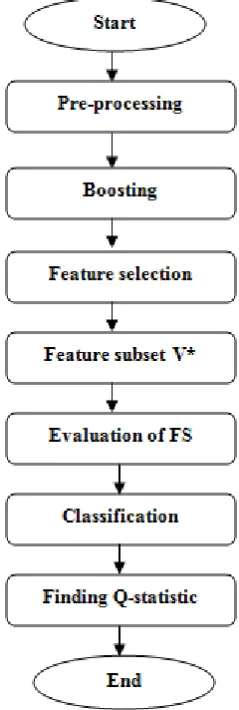
Fig 1 shows the overview of the proposed system. The weekly relevant features, irrelevant

features and redundant features are removed by the pre-processing method. Boosting is just a

re-sampling technique in the sample space. Four feature selection algorithm and classification

techniques used here to evaluate the results efficiently. Every high dimensional data has an

intrinsic challenge so the boosting technique is done to overcome the challenge with high

accuracy. The basic idea is to resample the data sets by splitting process in the sample space

and feature selection algorithm is applied. The number of splitting is denoted by b, depends

on the accuracy. So choice of b also plays a role in improving the accuracy of the

Figure 1: System Design.

IV. IMPLEMENTATION A. Pre-Processing

In high dimensional data the pre-processing needs to be done eminently because boosting

cannot be applied without removing redundant and irrelevant feature so that time complexity

is reduced.

1. Finding Week Relevant Feature by F-Test/T-Test

To perform pre-processing on numeric data both t-test and f-test can be applied. F-test can be

applied for more than two class labels while t-test can be applied for dataset containing only

two class labels. F-test is done by taking the variance test for each features µ1,µ2…µp where p

is the number features. Considering variance is equal as null hypothesis and not equal is

independent as alternate hypothesis the selection of feature is done. Here if two variance µ1,

µ2 are likely equal i.e., µ1- µ2 << 0.1 then the feature is irrelevant and it is eliminated or

2. Removing Irrelevant features by Discretization

The discretization technique is most commonly used in most of the Feature Selection

algorithm. It is the density estimation of feature in the high dimensional data with large

sample size as a whole dataset. It follows the marginal and joint probability mass function as

I(x1, x2) = ∑∑ f(x1, x2) log [f(x1, x2) / f(x1)f(x2)] (1)

After discretization if the MI = 0, Mutual Information value of feature, then feature contains

no valid information and in is removed from the dataset.

B. Boosting

Boosting is simply a re-sampling technique done in the sample space. For this booster

training sets is D divided into b partitions Di, i = 1, 2…b so that D = Ui=1b Di. From these Di’s

we obtain sp training subsets features Si such that Si = D-Di. For each of these Si feature

selection algorithm is applied to obtain V*, feature subset collection.

Algorithm 1: Boosterb

Input: Dataset D, FS algorithm s, Number of Partitions b

Output: Feature subset V*

Step 1: split D into b partitions Di, i=1, 2 …b Step 2: set V*= NULL

Step 3:for all Di

Step 4: Si = D- Di; /* remove Di from D */

Step 5: Vi = s (Si); /* obtain V by applying Si on s */ Step 6: V*= V* U Vi

Step 7: end for

Step 8: return V*

Initially the dataset is divided into b partitions and Si training subset is obtained for each Di.

This Si is applied for the feature selection algorithm and Vi is obtained to get feature subset.

Finally V* is obtained by union of all Vi. By applying this algorithm we obtain feature subset

V which contains only relevant feature with no redundancy. The number of partitions b plays

a key role and if b is larger more relevant features is obtained. If b is smaller redundancy will

C. Feature Selection

In this paper we applied four feature selection algorithms as minimum- redundancy-

maximal- relevance (mRMR), Fast Correlation Based Filter (FCBF), Fast clustering bAsed

feature Selection Algorithm (FAST) and mRMRe is the ensemble mRMR which is multiple

mRMR selections in parallel. All the four algorithms work well for discretized data. For

mRMR with large p eg.., P > 5000 the size of the selection m is fixed to 50. Smaller size (m <

30) gives lower accuracies and lower values of Q-statistic while larger size gives not much

improvement than m = 50. So m is fixed to 50.

Among the four, the most efficient one is mRMRe where it implicitly removes the

redundancy of the features. On the FCBF and FAST the explicit code is written for removing

redundancy.

The mRMRe is well supported for all real dataset. Here mRMR technique is extended with an

ensemble technique which is used for better explore of the feature subset collection and

robustness is highly achieved. These ensemble mRMR implementations outperform the

classical mRMR approach in terms of prediction accuracy. They identify genes more relevant

to the biological context with high accuracy and interpretation of various biological

applications. The parallelized functions included in the package show significant gains in

terms of run-time speed when compared with previously released packages.

D. Classification

To find the Q-statistic value we need classification accuracy. Here three classifiers used:

K-Nearest Neighbor (KNN), Naive Bayes (NB), Support Vector Machine (SVM). First

choosing the appropriate number of partitions b for Booster is considered. Then the relative

performance is evaluated as efficiency of Booster over the original FS algorithm is based on

the prediction accuracy and Q-statistic. Finally the Q-statistic was determined and accuracy

for the selected subset is shown high.

Algorithm 2: Evaluation process of FS

Input: FS algorithm, number of folds k, original dataset D and

K-folded data subsets Di, i= 1, 2 … k Output: accuracy ai , Vi*

Step 1: for all i

Step 3: Vi*Booster (Si) Step 4: ai  classifier (Di) Step 5: end for

Finally Q-statistic was determined using k-pairs of (Vi*,ai)

E. Finding Q-statistic

For evaluation of the three FS algorithms, with the corresponding boosters, initially k-fold

cross validation is applied for whole dataset. Here k training and testing subsets are obtained.

Booster process is applied to training process to get V* and testing sets for classification is

done. This process is repeated for the k pairs of training-test sets, and the value of the

Q-statistic is computed. Here k = 5 is used for all real datasets.

Q-statistic value is determined by the following statistics value.

(2)

(3)

F. Choice of b for Booster

The average size of |V*| increases rapidly to 15 as b increases to 5 but after 5 it do not vary

much. Booster accuracy and classification accuracy also increases rapidly up to b=5 after 5 it

varies slightly. Hence from the results, b= 5 is set. If b increases accuracy also increases. So

the value b plays a key factor for this proposed methodology.

V. RESULT ANALYSIS

This section describes the experimental results for different real datasets.

Table 1: Accuracy and Q-Statistic from Boosterb for the Four FS Algorithms and the Three Classifiers with b = 3 and 5.

b FAST FCBF mRMR mRMRe

SVM KNN NB SVM KNN NB SVM KNN NB SVM KNN NB

Accuracy %

3 90.2 91.8 89.9 91.3 92.4 89.3 91.1 91.4 87.3 93.3 92.4 91.1

5 92.3 92.7 91.2 93.8 92.0 91.2 93.4 92.4 89.9 94.4 92.9 90.8

100* Q 3 27.3 24.6 26.8 31.7 34.6 31.9 36.6 39.4 38.1 37.3 39.8 38.7

5 32.5 29.7 30.1 34.3 37.1 36.8 38.0 39.8 40.3 38.7 40.2 40.5

Table 1 shows Accuracy and Q-Statistic from Booster b for the Four FS Algorithms and the

Three Classifiers with b = 3 and b= 5. Here ensemble mRMR is well recognized for different

real datasets. Boosting technique helps the feature selection algorithm to increase the

accuracy of the classification and stability of the selected feature subsets. Especially in micro

array gene expression data it is necessary to apply boosting technique since it is used for

many biomedical applications. Table 2 and Table 3 shows Accuracies Obtained by the Three

Classifiers Based on the Features Selected by the Four FS Algorithms: FAST, FCBF, mRMR

and Q-Statistics Obtained by the Three Classifiers Based on the Features Selected by the Four

FS Algorithms: FAST, FCBF, mRMR respectively.

Table 2: Accuracies Obtained by the Three Classifiers Based on the Features Selected by the Four FS Algorithms: FAST, FCBF, and mRMR.

Dataset FAST FCBF mRMR mRMR

SVM KNN NB SVM KNN NB SVM KNN NB SVM KNN NB

B-cell1 0.92 0.97 0.95 0.99 0.92 0.98 0.94 0.99 0.91 0.95 0.99 0.93

Colon

cancer 0.88 0.95 0.93 0.97 0.94 0.91 0.98 0.93 0.96 0.98 0.95 0.96

Embryonal-

Tumors 0.94 0.91 0.88 0.94 0.99 0.91 0.98 0.95 0.93 0.99 0.99 0.97

Leukemia 0.93 0.94 0.82 0.98 0.92 0.97 0.94 0.96 0.90 0.96 0.98 0.97

Lung

cancer 0.91 0.91 0.94 0.82 0.84 0.86 0.95 0.97 0.92 0.95 0.97 0.96

Prostate 0.88 0.83 0.86 0.87 0.88 0.85 0.92 0.99 0.93 0.94 0.99 0.95

Breast

Cancer 0.99 0.91 0.95 0.94 0.96 0.90 0.94 0.91 0.98 0.96 0.92 0.99

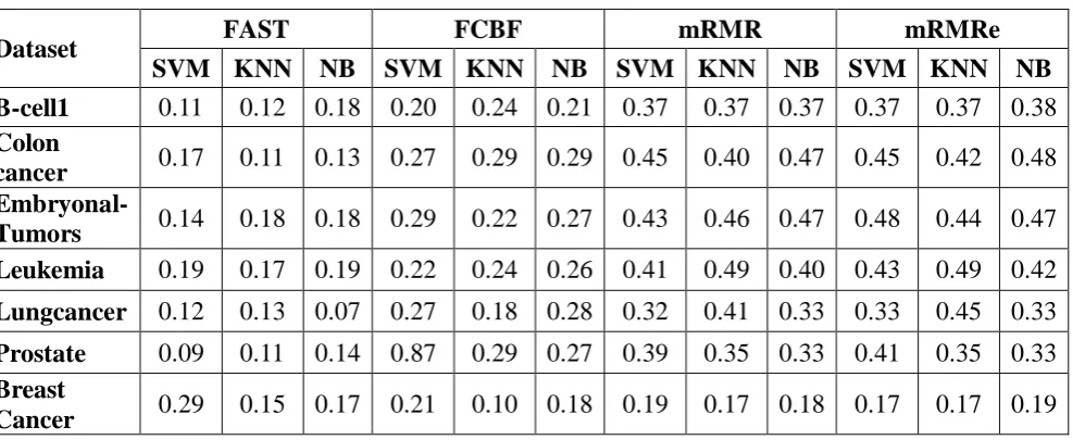
Table 3.Q-Statistics Obtained by the Three Classifiers Based on the Features Selected by the Four FS Algorithms: FAST, FCBF, and mRMR.

Dataset FAST FCBF mRMR mRMRe

SVM KNN NB SVM KNN NB SVM KNN NB SVM KNN NB B-cell1 0.11 0.12 0.18 0.20 0.24 0.21 0.37 0.37 0.37 0.37 0.37 0.38

Colon

cancer 0.17 0.11 0.13 0.27 0.29 0.29 0.45 0.40 0.47 0.45 0.42 0.48 Embryonal-

Tumors 0.14 0.18 0.18 0.29 0.22 0.27 0.43 0.46 0.47 0.48 0.44 0.47 Leukemia 0.19 0.17 0.19 0.22 0.24 0.26 0.41 0.49 0.40 0.43 0.49 0.42

Lungcancer 0.12 0.13 0.07 0.27 0.18 0.28 0.32 0.41 0.33 0.33 0.45 0.33

Prostate 0.09 0.11 0.14 0.87 0.29 0.27 0.39 0.35 0.33 0.41 0.35 0.33

Breast

VI. CONCLUSION

Here Q-statistics evaluates the performance of FS algorithm is for both stability for selected

subset and classification accuracy. The basic reason for improving accuracy is the boosting

not improve the accuracy value for some data sets. Hence boosting is done before feature

selection and increasing the value of b i.e., the number of partitions, results in increasing

accuracy value.

VII. REFERENCES

1. Z.I.Botev, J.F.Grotowski, and D.P.Kroese, “Kernel density estimation via diffusion,” The

Ann. Statist., 2010; 38(5): 2916–2957.

2. G.Brown, A. Pocock, M. J. Zhao, and M. Lujan, “Conditional likelihood maximization: A

unifying framework for information theoretic feature selection,” J. Mach. Learn. Res.,

2012; 13(1): 27–66.

3. B.C.Christensen, E.A.Houseman, C.J.Marsit, S.Zheng, M. R.Wrensch, H. H. Nelson, M.

R. Karagas, J. F. Padbury, R. Bueno, D.J. Sugarbaker, R.F. Yeh, J.K. Wiencke, and K.T.

Kelsey, “Aging and environmental exposures alter tissue-specific DNA methylation dependent upon CPG island context,” PLOS Genetics, 2009; 5(8): e1000602.

4. Z.He and W.Yu, “Stable feature selection for biomarker discovery,” Comput. Biol.

Chem., 2010; 34(4): 215–225.

5. M. Hilario and A.Kalousis, “Approaches to dimensionality reduction in proteomic

biomarker studies,” Briefings Bioinf., 2008; 9(2): 102–118.

6. Q. Hu, L. Zhang, D. Zhang, W. Pan, S. An, and W. Pedrycz, “Measuring relevance

between discrete and continuous features based on neighborhood mutual information,”

Expert Syst. With Appl., 2011; 38(9): 10737–10750.

7. J.Hua, W.D.Tembe, and E.R.Dougherty, “Performance of feature-selection methods in

the classification of high-dimension.

8. D.Dernoncourt, B.Hanczar, and J.D.Zucker, “Analysis of feature selection stability on

high dimension and small sample data, “Comput. Statist. Data Anal., 2014; 71: 681–693.

9. R.V.Jorge and A.E.Pablo, “A review of feature selection methods based on mutual

information,” Neural Comput. Appl., 2014; 24(1): 175–186.

10.A.Kalousis, J.Prados, and M.Hilario, “Stability of feature selection algorithms: A study

on high-dimensional spaces,” Knowl. Inf. Syst., 2007; 12(1): 95–116.

11.I.Kojadinovic, “Relevance measures for subset variable selection in regression problems

based on k-additive mutual information,” Comput. Statist. Data Anal., 2005; 49(4):

1205–1227.

12.D.Koller and M.Sahami, “Toward optimal feature selection,” in Proc. 13th Int. Conf.

13.L. I. Kuncheva, “A stability index for feature selection,” in Proc. Artif. Intel. Appl., 2007;

pp. 421–427.

14.H. Liu, J. Li, and L.Wong, “A comparative study on feature selection and classification

methods using gene expression profiles and proteomic patterns,” Genome Informatics

Series, 2002; 13: 51–60.

15.H. Liu, M. Xu, H. Gu, A. Gupta, J. Lafferty, and L. Wasserman, “Forest density

estimation,” The J. Mach. Learn. Res., 2011; 12: 907–951.

16.R. S. Marko, and I. Kononenko, “Theoretical and empirical analysis of ReliefF and

RReliefF,” Machine learning, 2003; 53 (1–2): 23–69.

17.P. Somol and J. Novovicova, “Evaluating stability and comparing output of feature

selectors that optimize feature subset cardinality,” IEEE Trans. Pattern Anal. Mach. Intel.,

Nov. 2010; 32(11): 1921–1939.

18.Q. Song, J. Ni, and G. Wang, “A fast clustering-based feature subset selection algorithm

for high-dimensional data,” IEEE Trans. Knowl. Data Eng., Jan. 2013; 25(1): 1–14.

19.A. I. Su, M. P. Cooke, K. A. Ching, Y. Hakak, J. R. Walker, T. Wiltshire, A. P. Orth, R.

G. Vega, L. M. Sapinoso, A. Moqrich, A.Patapoutian, G. M. Hampton, P. G. Schultz, and

J. B. Hogenesch, “Large-scale analysis of the human and mouse transcriptomes,” Proc.

Nat. Acad. Sci. USA, 2002; 99(7): 4465–4470.

20.Y. Sun, S. Todorovic, and S. Goodison, “Local-learning-based feature selection for

high-dimensional data analysis,” IEEE Trans. Pattern Anal. Mach. Intel., Sep. 2010; 32(9):

1610–1626.

21.K. M. Ting, J. R. Wells, S. C. Tan, S. W. Teng, and G. I. Webb,“Feature-subspace

aggregating: Ensembles for stable and unstable learners,” Mach. Learn., 2011; 82(3):