UDC: 519.642:532
On Accuracy of the Element-Free Galerkin (EFG) Method in Modeling
Incompressible Fluid Flow
I. Vlastelica1,2, V. Isailović3, T. Djukić4, N. Filipović3,4, M. Kojić*3,5,6
1 Technical High School, Čačak, Serbia
2 Faculty of Information Technologies, Belgrade, Serbia
3 Research and Development Center for Bioengineering ‘BIOIRC’, Kragujevac, Serbia
[email protected]; [email protected]
4 Faculty of Mechanical Engineering, University of Kragujevac, Serbia
5 Harvard School of Public Health, Boston, USA
6 Department of Biomedical Engineering, University of Texas Medical Center at Houston, USA
*Corresponding author
Abstract
Element-free Galerkin method (EFG) has been introduced in the nineties of last century (see e.g. Belytschko et al. 1994, 1996). It represents a mesh-free method, particularly suitable for problems where the FE method would need a remeshing procedure. The EFG has been mainly used in solid mechanics for problems involving change of the boundary, as in case of fracture propagation.
We have investigated applicability of the EFG in modeling incompressible fluid flow, especially the solution accuracy when various numbers of free points and integration schemes are employed. In this report we present our findings by analyzing solution of simple fluid flow examples: flow on a plate and flow in a cavity.
Keywords: Element-free Galerkin method, accuracy of fluid flow solutions, variation of number of free points, flow on a plate, flow in a cavity
1. Introduction
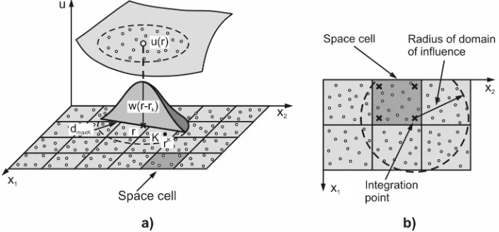
The element free-Galerkin method (EFG) has been introduced to overcome the difficulties arising in the FE method applications (see e.g. Belytschko et al. 1994, 1996). The EFG idea consist basically in that a spatial field is interpolated over a certain points, called free-points, which do not belong to a mesh, as in the FE method. The interpolation relies on the vicinity criterion, i.e. a value of the interpolated quantity at a point within the modeling domain is affected by values at free points within a surrounding domain of a specified size. The key term in this interpolation is a weight function which decays with the distance, as graphically illustrated in Fig. 1.
The EFG is not totally mesh-free because a space mesh is required to perform integration over subdomains called EFG cells. The space integration is performed in a usual manner, as in the FE method, over integration points. A contribution to the governing matrices and vectors used to express balance laws, evaluated at an integration point, is added to the corresponding terms of the matrices and vectors of the discretized system of equations. During the solution procedure the number of free points belonging to an integration point might change, as well as the space cells, what offers a significant flexibility in modeling.
Fig. 1. Discretization of a function u (r) by the EFG method. (a) Schematic of discretization into space cells and use of free points ( (wr r− K) is the weight function, K is a free point,
maxK
d
defines the size of the domain of influence for the weight function w(
r r− K)
); (b) Space cell used for integration and domain of influence around the integration point. Accordingto Kojic et al. (2008a).
We summarize the basic equations of the EFG in the next section, followed by the incremental equations of balance for incompressible fluid; then we present accuracy analysis on two examples, and finally give concluding remarks at the paper.
2. Fundamental relations of the EFG
( )
m( ) ( )
T( ) ( )
j j j
u r =
∑
p r a r ≡p r a r (1)where pj
( )
r are the components of the base vector p r( )
, as monomials in the coordinates of(
x y z, ,)
r so that the basis is complete; it is set that the component p1=1; and m is the basis
size. We need to determine the coefficients aj
( )
r and we proceed as shown further in the text. The linear and quadratic bases for one-dimensional space are( )
[ ]
1, , linear, 2;( )
1, , 2 , quadratic, 3T = x m= T =⎡ x x ⎤ m=
⎣ ⎦
p r p r (2)
and for the 2D space we have
( )
[
]
( )
2 21, , , linear 3
1, , , , , quadratic 6
T
T
x y m
x y x xy y m
= =
⎡ ⎤
=⎣ ⎦ =
p r
p r (3)
The coefficients aj
( )
r are determined by minimizing a weighted quadratic form(
) ( )
( )
21
n
K T K K
K
J w U
=
⎡ ⎤
=
∑
r r− ⎣p r a r − ⎦ (4)where K denotes the free point number with the position vectors rK and with the value of the
function UK; w
(
r r− K)
is a weight function which decreases with the distance between amaterial point with position vector r and the free point K (see Fig.1); and n is the number of free points in the domain of influence around the material point. From the minimization of J
with respect to the coefficients aj
( )
r , we obtain the following system of equations:(
)
1
2n K K K K 0, sum on : 1, 2,...,
j j i
K i
J w p a U p j j m
a =
∂
= − = =
∂
∑
(5)where wK ≡w
(
r r− K)
, K( )
K j jp ≡ p r . We further write this system of equations as
0, sum on and : 1, 2,..., ; 1, 2,..., K
ij j iK
A a −B U = K j K= n j= m (6)
where the matrices A and B are:
1
; , no sum on
n
J J J K K
ij i j iK i
J
A w p p B p w K
=
=
∑
= (7)The matrices A and B are of order m m× andm n× , respectively. By solving the system (6) we obtain the coefficients aj
( )
r :( )
1( )
(
1)
1
; or n K
j jK K a U − − = = =
∑
a r A BU r A B (8)
Substitution of a r
( )
from (8) into (1) gives the approximation for the function u( )
r as( )
1( )
1
n
T K
K K
u − U
=
= =
∑
Φwhere the interpolation function ΦK
( )
r corresponding to the free point K, is( )
(
1)
1
m
K jK j
j
p − =
Φ r =
∑
A B (10)The form (9) can further be used in all derivations of expressions needed in the governing equations, either for solid or fluid (see Section 3). Details how derivatives of the interpolation with respect to a Cartesian coordinates can be found elsewhere (e.g. Vlastelica 2003; Kojic et al. 2006, 2008a,b).
We further give two expressions for the weight functions: exponential and polynomial (Belytschko et al. 1994). The exponential form is
( )
(
)
(
(
)
)
2 2 max max 2 2 max maxexp / exp /
,
1 exp /
0,
k k
J J
J J
J k k
J J
J J
d c d c
d d
w d d c
d d ⎧ ⎡− ⎤− ⎡− ⎤ ⎣ ⎦ ⎣ ⎦ ⎪ ≤ ⎪ =⎨ − ⎡⎣− ⎤⎦ ⎪ ⎪ ≥ ⎩ (11)
and the polynomial form is
( )
2 3 4
max
max max max
max
1 6 8 3 ,
0
J J J
J J J
J J J J
J J
d d d
d d
w d d d d
d d ⎧ ⎛ ⎞ ⎛ ⎞ ⎛ ⎞ ⎪ − ⎜ ⎟ + ⎜ ⎟ − ⎜ ⎟ ≤ = ⎨ ⎝ ⎠ ⎝ ⎠ ⎝ ⎠ ⎪ > ⎩ (12)
where J
J
d = −r r is the distance between the material point and the free point J; dmaxJ is the
domain of influence for the weight function wJ; k is the parameter (in the examples here we
use k=1); and
max K J for all free points
c=α r −r (13)
where 1≤ ≤α 2 is recommended.
3. Incremental-iterative EFG equations of balance for incompressible fluid
Here, we summarize a derivation of EFG equations of balance used in an incremental-iterative solution procedure. The steps in this derivation are analogous to those in the FE method (Kojic et al. 2008a).
The fundamental equation of balance of linear momentum is given as
. V 0 1,2,3; sum on : 1, 2,3
i ik
i k k i
i k
v p
v v f i k k
t x x
τ
ρ⎛⎜∂ + ⎞⎟+∂ −∂ − = = =
∂ ∂ ∂
⎝ ⎠ (14)
where ρ is fluid density, vi are velocity components, p is pressure, τik are viscous stresses, and V
i
f are components of a body force (per unit volume). Now, we adopt interpolation for velocity and pressure as
, or K; sum on , 1,2,...., ; 1, 2,3
i K i
v V K K n i
= = Φ = =
v ΦV (15)
ˆ , or K, sum on , 1,2,...., K
p=ΦP p= Φ P K K= n (16)
where V is the vector of velocities at free points in the domain of influence – its transpose is
1 2 1 2 1 2
1 1... ;1 2 2... ;2 3 3... 3
T⎡V V V V Vn V V Vn Vn⎤
⎣ ⎦
V ; and P the vector of pressures at free points.
We next apply the Galerkin method according to which we multiply (14) by the interpolation functions
(
, K)
K
Φ r r (and use the Gauss theorem) to obtain the following balance equation in a matrix form
ˆ
vv vp v τ
+ + = −
MV K V K P F F (17)
where the matrices can be written in component form as
[
KJ]
ii K JV
M =
∫
ρΦ Φ dV (18)( )
ˆvv KJ K J j, j iiV ii
v dV
ρ
⎡ ⎤
⎡ ⎤ =⎢ Φ Φ ⎥
⎣ K ⎦ ⎣
∫
⎦ (19)( )
vp KJ ii K i, ˆJ VdV
⎡ ⎤ = − Φ Φ
⎣ K ⎦
∫
(20)The capital indices represent the free point numbers, while the indices i and j denote the coordinate numbers (=1,2,3). The terms of the nodal force vectors are:
( )
(
)
,( )
,V
v Ki K i K ij ij j Ki K j ij
V S V
f dV pδ τ n dS τ τ dV
= Φ
∫
+ Φ −∫
+ = Φ∫
F F (21)
where V is the volume the considered domain, and S is the surface bounding this domain. Note that the integral over the domain surface results in the force vector Fvi; and summation of these vectors during the assemblage procedure leads to the cancellation, so that only the surface forces at the external boundaries remain.
A more common form of equation (17) is obtained with substituting the constitutive law for the viscous stress:
(
, ,)
2
ij eij vi j vj i
τ = μ =μ + (22)
where μ is the viscosity coefficient. Then equation (17) becomes
vv vp v
+ + =
MV K V K P F (23)
where now the matrix Kvv is
( )
ˆvv KJ KJ ii KJ ii ii K Kμ
⎡ ⎤ =⎡⎣ ⎤⎦ +⎡⎣ ⎤⎦
⎣ K ⎦ (24)
width
, ,
K j J j KJ ii
V
Kμ μ dV
⎡ ⎤ = Φ Φ
⎣ ⎦
∫
(25)( )
(
,)
V
v Ki K i K ij i j j
V S
N f dV N pδ μv n dS
=
∫
+∫
− +F (26)
Equation (23) represents the Navier-Stokes equation in the EFG formulation.
To make the system of balance equations complete, we need to employ the continuity equation, now the continuity equation which for incompressible fluid is:
, 0
i i
v = , or 1 2 3
1 2 3
0
v v v x x x
∂ +∂ +∂ =
∂ ∂ ∂ (27)
Multiplying this equation by the interpolation functions ΦˆK, a weak form of the continuity equationis obtainedas
,
ˆ J 0, or T 0
K J j j vp
V
dV V
⎛ ⎞
Φ Φ = =
⎜ ⎟
⎝
∫
⎠ K V (28)where the matrix Kvp is given in (20).
The system of equations (23) (or (17)) and (28) represent the system of EFG equations which can be assembled in a usual manner. The system is nonlinear since the matrix Kvv is
nonlinear: it contains the velocity as the coefficient in KJ
ii
K
⎡ ⎤
⎣ ⎦ . Therefore, an iterative scheme
(see e.g. Kojic et al. 2008a) must be employed. For a time step ‘n’ we obtain the following iterative form
( 1)
( 1) ( 1)
1 ( )
( )
( 1)
1 1
1 ( 1)
1
1
1 1
0 0 0
i i i n i vv vp i T vp i
n n n
n i vv vp ext n T vp t t t − − − + − + + + − + ⎡ + ⎤⎧Δ ⎫ ⎢Δ ⎥⎨ ⎬= ⎢ ⎥ Δ⎩ ⎭ ⎢ ⎥ ⎣ ⎦ ⎡ + ⎤⎧ ⎫ ⎧ ⎫ ⎧ ⎫ ⎢ ⎥⎪ ⎪ ⎪ ⎪ − Δ + Δ ⎨ ⎬ ⎢ ⎥⎨ ⎬ ⎨ ⎬ ⎩ ⎭ ⎢⎣ ⎥⎦⎪⎩ ⎪ ⎪⎭ ⎩ ⎪⎭
M K K V
P
K 0
M K K V M V
F P K (29) where
(
)
1 ( 1) 1 ( 1) 1 ( 1)
n i n i n i
vv KJ KJ ii KJ ik
ik K J
+ − + − + −
⎡ ⎤ =⎡⎣ ⎤⎦ +⎡⎣ ⎤⎦
⎣ K ⎦ (30)
and
1 ( 1) 1 ( 1)
,
n i n i
KJ ik K i k J V
J ρ v dV
+ − + −
⎡ ⎤ = Φ Φ
⎣ ⎦
∫
(31)4. Examples
In this section we present two examples to demonstrate effects of number of free points within an EFG cell and number of integration points on solution accuracy.
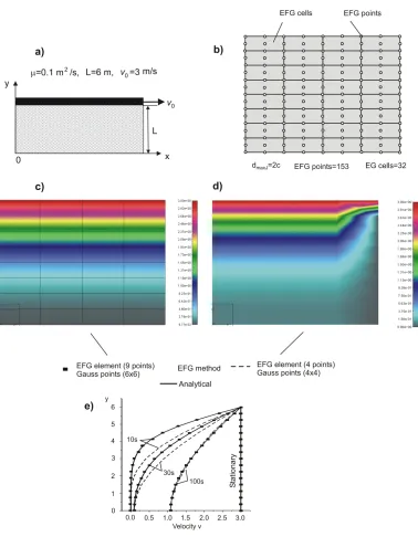
4.1Example 1 - Unsteady flow on a plate
We consider a 2D flow of incompressible flow caused by motion of a plate (Fig.2a). The dimension orthogonal to the plate is large (in the analytical model it is taken as infinity). Motion starts from the rest and motion of the plate by constant velocity v0 propagates into the fluid
producing the ultimate uniform fluid velocity in the vicinity of the plate, see the velocity profile in Fig. 2e denoted as stationary state.
EFG model is shown in Fig. 2b. We used the EFG cells shown in the figure and changed number of free points within each cell. We also used various number of integration points. In all these analyses the domain of influence was taken to be domain of the EFG cell.
The results are shown in Figs. 2c,d,e. Figures 2c and 2d show velocity fields for time 30s
for 9 free points in EFG cells and 6 6× Gauss integration, and 4 free points in EFG cells and4 4× Gauss integration, respectively. The linear basis (see (13)) is used for the velocity field and the exponential function (11) with dmaxJ =2c. It can bee seen that the field with more
Fig. 2. Modeling of unsteady flow on a plate. (a) Geometry and material data; (b) EFG model; (c) and (d) Velocity field at time t=30s: (c) 9 free points in EFG cells and 6 6× Gauss integration, (d) 4 free points in EFG cells and4 4× Gauss integration; (e) Velocity profiles during evolution of flow from the resting state to stationary conditions, EFG and analytical
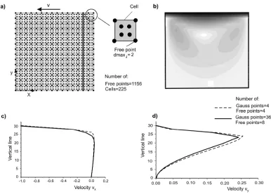
4.2 Example 2 - Flow in a cavity
In this example we analyze fluid flow in a box (cavity). Motion of the fluid is caused by motion of the top boundary by constant velocity v, Fig. 3a. This example has been served as a benchmark example for testing solution methods of incompressible fluid flow, such as the finite element method (FE), dissipative particle dynamics (DPD), or multiscale procedure – coupling the DPD and FE methods (see, e.g. Kojic et. al. 2008a,b).
Here, we modeled this fluid flow by the EFG method. The mesh of the EFG cells and 8 free points belonging to a cell is shown in Fig. 3a. The linear basis (see (3)) is used for the velocity field and the exponential function (11) with
d
max,J=
2
c
.The fluid is initially at rest and the flow tends to ultimate stationary state.Fig. 3. EFG model of flow in a cavity. (a) Geometry, mesh of EFG cells and free points within a cell; (b) Field of velocity for time t=10 s.
5. Conclusions
We explored applicability of the EFG method to modeling incompressible fluid flow. The aim of this report also was to investigate solution accuracy when number of EFG free points changes within a cell. Also, solutions are compared when the number of integration points is changed. Our findings are illustrated on two examples.
It can be concluded that an increased number of free points per cell with increased number of integration points lead to more accurate results. From these EFG modeling features it follows that to improve solution accuracy, more computing efforts are required and therefore the method might be computationally inefficient. On the other hand, the EFG method have advantages in modeling problems where the FE method would need a remeshing.
Acknowledgements
The authors acknowledge support of the Ministry of Science of Serbia, grant OI144-2/08; and City of Kragujevac, Contract 1224/08.
References
Belytschko T, Lu YY, Gu L (1994). Element-free Galerkin methods, Int. J. Num. Meth. Engrg., 37, 229-256.
Belytschko T, Krongauz Y, Organ D, Fleming M, Krysl P (1996). Meshless Methods: An overview and recent developments, Comp. Meth. Appl. Mech. Engrg., 139, 3-47.
Kojic M, Filipovic N, Tsuda A (2006). A multiscale method for bridging dissipative particle dynamics and Navier-Stokes finite element equations for incompressible fluid and its application in biomechanics. Proc. First South-East European Conference on Comp. Mechanics (Eds. M. Kojic and M. Papadrakakis), Kragujevac, Serbia.
Kojic M, Filipovic N, Stojanovic B, Kojic N (2008a). Computer Modeling in Bioengineering – Theory, Examples and Software, J. Wiley and Sons.
Kojic M, Filipovic N, Tsuda A (2008b). A mesoscopic bridging scale method for fluids andcoupling dissipative particle dynamics with continuum finite element method, Comp. Meth Appl. Mech. Eng., 197, 821-833.