Efficient Numerical Computations of Soft Constrained Nash Strategy for Weakly Coupled Large-Scale Systems

Efficient Numerical Computations of

Soft Constrained Nash Strategy for

Weakly Coupled Large-Scale Systems

Muneomi Sagara, Hiroaki Mukaidani, Toru Yamamoto

Graduate School of Education, Hiroshima University, Higashihiroshima, JAPAN Email:{d074978, mukaida, yama}@hiroshima-u.ac.jp

Abstract— In this paper, a high-order soft constrained Nash

strategy for weakly coupled large-scale systems is investi-gated. In order to solve the cross-coupled sign-indefinite algebraic Riccati equations (CSAREs) corresponding to strategy, the iterative algorithm on the basis of the Newton’s method is first applied. Second, the recursive algorithm for solving the CSAREs is also established to reduce the amount of algebraic computation as compared with the Newton’s method. Using these iterative solutions, a high-order soft-constrained Nash strategy is designed. As a result, it is proved that the proposed high-order approximate equilibrium strategies achieve better performance. Finally, in order to demonstrate the efficiency of the algorithm, a numerical example is given.

Index Terms— soft constrained Nash strategy, weakly

cou-pled large-scale systems, cross-coucou-pled sign-indefinite al-gebraic Riccati equations (CSAREs), Newton’s method, recursive algorithm, high-order approximate equilibrium strategies

I. INTRODUCTION

The control problems of weakly coupled large-scale systems have been studied by several researchers (see [3], [4] and references therein). In practice, it is known that such systems are represented by multi-area power systems [3], distillation columns [11] and cold-rolling mills [12]. They are widely used to represent the system dynamics.

Linear quadratic Nash games and their applications have been widely investigated in many literatures (see e.g. [5], [6] for weakly coupled large-scale systems). In the deterministic case, a guaranteed cost problem for the state feedback strategies of nonzero-sum differential games involving multiple players was investigated [13]. The Nash strategy was applied to systems using active magnetic bearings: it has successfully reduced the error dynamics induced by linearization [14]. However, robust Nash equilibrium in deterministic uncertain systems has not been investigated thus far. In contrast, robust equilibria in indefinite linear quadratic differential games under a deterministic disturbance input affecting the systems have been discussed [1]. The results in [1] are very elegant This paper is based on “High-Order Approximation of Soft Con-strained Nash Strategy for Weakly Coupled Large-Scale Systems,” by H. Mukaidani, which appeared in the Proceedings of the 2007 IEEE International Conference on Systems, Man, and Cybernetics, Montreal, Canada, October 2007. c2007 IEEE.

This work was supported in part by the Electric Technology Research Foundation of Chugoku of Japan.

in theory and it is easy to obtain a strategy pair by solving the cross-coupled sign-indefinite algebraic Riccati equations (CSAREs). In [2], the numerical algorithm that is based on the calculation of the eigenstructure for solving the soft-constrained Nash equilibria has been developed. However, the scalar case has only been con-sidered. In addition, the convergence rate is unclear. On the other hand, the Newton-type algorithm for solving the CSAREs has been established [7], [8]. Although the Newton’s method guarantees the fast convergence, this existing algorithm has to utilize two fixed-point iterations to attain the reduced-order computations. Therefore, the large amount of computation and CPU time are needed. Moreover, the degradation of the cost performance under the use of the strategies that is based on the iterative solution has not been investigated in [7].

This paper investigates the soft-constrained Nash games for the weakly coupled large-scale systems that attains the high-order approximation by using the iterative solutions. The main contribution is to propose a new high-order approximation strategy that is based on the solution of the CSAREs via the Newton’s method with the appropriate initial guess. As a result, although the CSAREs has the sign-indefinite quadratic form as compared with the exist-ing results [5], [6], the convergence solutions satisfy the required properties such as the stability and the positive-definiteness. Thus, it is proved that the proposed strategy that is based on the iterative solutions with a few iterations achieves a high-order approximation of better equilibrium. As another important contribution, the recursive algorithm for solving the CSAREs is given. It is shown that the proposed algorithm converges to the exact solution with linear rate. In addition, since only low-order systems are involved in algebraic computations, the amount of computations required does not increase per iterations as compared with the Newton’s method [7], [8]. As a result, the reduction of the CPU time is guaranteed. Finally, in order to demonstrate the efficiency of the proposed design methodology, a numerical example is included.

vector of the matrix_M. The space ofRk-valued functions that are quadratically integrable on(0, ∞)is denoted by Lk₂(0, ∞).

II. PROBLEMFORMULATION

Consider the weakly coupled large-scale linear systems with_N-players

˙

xi(t) =Aiixi(t) +Biiui(t) +ε N

j=1, j=i Aijxj(t)

+_εN j=1, j=i

Bijuj(t) +Eiiwi(t) +ε N

j=1, j=i

Eijwj(t),

xi(0) =x0i, i= 1, ... , N, (1) where _xi ∈ Rni_{, i} = 1_{, ... , N represent i-th state}

vectors. _ui ∈ Rmi_{, i} = 1_{, ... , N represent i-th}

control inputs. _wi ∈ Rki_{, i} = 1_{, ... , N represent i}

-th disturbance vectors. _ε denotes a small positive weak coupling parameter which connect the other subsystems.

Let us introduce the partitioned matrices

Aε:= ⎡ ⎢ ⎢ ⎢ ⎣

A11 εA12 · · · εA1N εA21 A22 · · · εA2N

..

. ... . .. ... εAN1 εAN2 · · · ANN

⎤ ⎥ ⎥ ⎥ ⎦,

Biε:= ⎡ ⎢ ⎢ ⎢ ⎣

ε1−δ1i_B

1i ε1−δ2i_B2i

.. . ε1−δNi_BNi

⎤ ⎥ ⎥ ⎥

⎦, δij :=

0 (_i=_j) 1 (_i=_j) ,

Eε:= ⎡ ⎢ ⎢ ⎢ ⎣

E11 εE12 · · · εE1N εE21 E22 · · · εE2N

..

. ... . .. ... εEN1 εEN2 · · · ENN

⎤ ⎥ ⎥ ⎥ ⎦.

By using above relations, the system (1) can be changed as

˙

x(t) =Aεx(t) + N

i=1

Biεui(t) +Eεw(t), (2)

where

x(t) := x1(t)T · · · xN(t)T T ∈Rn¯, ¯n:= N

i=1 ni,

w(t) := w1(t)T · · · wN(t)T T ∈R¯k, ¯k:= N

i=1 ki.

The cost performance for each strategy subset is defined by

Ji(u1, ... , uN, w, x(0)) =

_∞

0

xT(t)Qiεx(t) +uTi(t)Riiui(t)

+µ N

j=1, j=i

uT_j(t)Rijuj(t)−wT(t)Viµw(t)

dt,(3)

where

Qiε= ⎡ ⎢ ⎢ ⎢ ⎣

ε1−δi1_{Qi1 εQi12} · · · _εQi1N εQT_i12 ε1−δi2_Q

i2 · · · εQi2N ..

. ... . .. ... εQTi1N εQTi2N · · · ε1−δiNQiN

⎤ ⎥ ⎥ ⎥ ⎦

∈R¯nׯn_,

Rii=RTii >0∈Rmi×mi, Rij=RTij ≥0∈Rmj×mj, Viµ =block diagµ−(1−δi1)_V

i1 · · · µ−(1−δiN)ViN

≥0∈Rkׯ ¯k_{, i, j}= 1_{, ... , N.}

The state weight matricesQiεis symmetric and assumed to be sign-indefinite [2]. Furthermore, it should be noted that _µ denotes a small positive parameter which is the same order for the parameter _ε. That is, the following assumption is made.

Assumption 1: The ratio of the small positive

parame-ters εand µis bounded by some positive constants ˜k. 0_<˜_k:=µ

ε <∞. (4)

Although it seems that this assumption is conservative, it will not affect the main contribution from the practical points of view.

A. Soft Constrained Nash Equilibrium Strategy

For the matrices _Aε, _Biε,_i= 1_{, ... , N}, the setF_N is defined by

FN :=

(_{F1ε, ... , FNε})|Aε+ N

j=1

BjεFjε is stable.

.

The soft constrained Nash equilibrium strategy pair (F₁∗_ε, ... , F_Nε∗ ) is defined as satisfying the following conditions [2].

¯

Ji(u∗1, ... , u∗N, x(0))

≤J¯i(u∗1, ... , ui, ... , u∗N, x(0)), i= 1, ... , N, (5) where _ui:=_ui(_t) =_Fiεx(_t),

¯

Ji(F1εx, ... , FNεx, x(0)) := sup

w∈L¯k

2(0,∞)

Ji(F1εx, ... , FNεx, w, x(0)),

Ji(F1εx, ... , FNεx, w, x(0))

= _∞

0

xT(t)[Qiε+FiεTRiiFiε+µ N

j=1, j=i

FjεTRijFjε]x(t)

−wT(t)Viµw(t)

dt,

for all x(0) and for all(F1ε, ... , FNε)that satisfy (F1∗ε, ... , Fi−∗ 1ε, Fiε, Fi∗+1ε, ... , FNε∗ )∈FN.

It should be noted that the following assumption guaran-tees the existence of the admissible strategy.

Assumption 2: Each player uses the linear feedback

This assumption is imposed on each player restrictively. In other words, it is assumed that each player on the subsystem take a stable strategy. If such conditions are not met, the overall systems would be not asymptotically stable.

B. CSAREs

Using the fact studied by [2], the soft constrained feedback Nash equilibrium is given below.

Lemma 1: [2] Assume that there exist _N real sym-metric matricesPiε and Wiε, such that

Gi(P1ε, ... , PNε)

:=_Piε ⎛

⎝_Aε−N j=1

SjεPjε ⎞ ⎠+

⎛

⎝_Aε−N j=1

SjεPjε ⎞ ⎠ T

Piε

+PiεSiεPiε

+µ N

j=1, j=i

PjεSijεPjε+PiεMiµPiε+Qiε= 0, (6)

where Siε :=BiεR−ii1BTiε, Sijε :=BjεR−jj1RijR−jj1BjεT, Miµ :=EεV_iµ−1EεT.

Aε− N

j=1

SjεPjε+MiµPiε is stable for i = 1, ... , N,

Aε− N

j=1

SjεPjε is stable,

Wiε ⎛

⎝_Aε−N j=1, j=i

SjεPjε ⎞ ⎠+

⎛

⎝_Aε−N j=1, j=i

SjεPjε ⎞ ⎠ T

Wiε

−WiεSiεWiε+µ N

j=1, j=i

PjεSijεPjε+Qiε≥0. (7)

Define the_N-tuple(_F1∗_{ε, ... , FNε}∗ )by

ui∗(t) :=Fiε∗x(t) =−Rii−1BiεTPiεx(t), i= 1, ... , N.(8) Then, (F₁∗_ε, ... , F_Nε∗ ) ∈ FN and this N-tuple is a soft constrained Nash equilibrium. Furthermore,

¯

Ji(F1∗εx, ... , FNε∗ x, x(0)) =x(0)TPiεx(0).

It should be noted that if _Qiε ≥ 0 and _Sijε ≥ 0 for all i = 1, ... , N, the matrix inequality (7) is trivially satisfied with Wiε = 0 [2]. Then, only the CSAREs (6) should be solved.

In the following analysis, the basic assumption is needed.

Assumption 3: [2] The triples(Aii, Bii, √Qii), i= 1, ... , N are stabilizable and detectable.

III. ASYMPTOTIC STRUCTURE OFCSARES Firstly, in order to obtain the strategy that is based on the numerical solutions, the asymptotic structure of the CSAREs (6) is established. Since Aε, Siε,Sijε and Miµ include the term of the small parameters ε and µ, the solution _Piε of the CSAREs (6), if it exists, must contain these parameters. Moreover, it should be noted

that two parameters_εand_µare the same magnitude such that Assumption 1 holds. Taking these facts into account, the solution Piε of the CSAREs (6) with the following structure is considered [4–6].

Piε

:= ⎡ ⎢ ⎢ ⎢ ⎣

ε1−δi1_{Pi1 εPi12} · · · _εPi1N εP_iT₁₂ ε1−δi2_Pi2 · · · _εPi2N

..

. ... . .. ... εP_iT_1N εP_iT_2N · · · ε1−δiN_PiN

⎤ ⎥ ⎥ ⎥

⎦∈Rnׯ n¯.

Substituting the matrices _Aε, _Siε, _Sijε, _Miµ, _Qiε and Piε into the CSAREs (6), letting ε= 0 and µ= 0, and partitioning the CSAREs (6), the following reduced-order algebraic Riccati equations (AREs) are obtained, where

¯

Pii, i= 1, ... , Nbe the0-order solutions of the CSAREs (6) asε=µ= 0.

¯

PiiAii+ATiiP¯ii−P¯ii(Sii−Mii) ¯Pii+Qii= 0, (9) where Sii:=BiiR−ii1BiiT andMii :=EiiVii−1EiiT.

In order to guarantee the existence of a positive semidefinite stabilizing solution of the ARE (9), the following condition is assumed.

Assumption 4: The ARE (9) has a positive semidefinite

stabilizing solution such that _Aii−_SiiP¯_ii is stable. The asymptotic expansion of the CSAREs (6) at _ε = µ= 0 is described by the following lemma [7], [8].

Lemma 2: Under Assumptions 1-4, there exist the

small constants σ∗ and ρ∗ such that for all ε∈(0, σ∗) andµ∈(0, ρ∗), the CSAREs (6) admits a unique positive semidefinite solutionP_iε∗ that can be written as

Piε:=Piε∗ = ¯Pi+O(ε)

=block diag 0 · · · _P¯_ii · · · 0 +_O(_ε)_. (10)

IV. NEWTON’SMETHOD FORSOLVINGCSARES In order to obtain the solution of CSAREs (6), the following useful algorithm is given.

P_iε(k+1) ⎛

⎝_Aε−N j=1

SjεPjε(k)+MiµPiε(k) ⎞ ⎠

+ ⎛

⎝_Aε−N j=1

SjεPjε(k)+MiµPiε(k) ⎞ ⎠ T

Piε(k+1)

−

N

j=1, j=i

P_jε(k+1)SjεPiε(k)− N

j=1, j=i

P_iε(k)SjεPjε(k+1)

+µ N

j=1, j=i

P_jε(k+1)SijεPjε(k)+µ N

j=1, j=i

P_jε(k)SijεPjε(k+1)

+ N

j=1, j=i

Pjε(k)SjεPiε(k)+ N

j=1, j=i

Piε(k)SjεPjε(k)

+_Piε(k)_SiεPiε(k)−µ N

j=1, j=i

Pjε(k)SijεPjε(k)

where

P_iε(k):= ⎡ ⎢ ⎢ ⎢ ⎢ ⎣

ε1−δi1_P(k)

i1 εPi(12k) · · · εPi(1kN) εP_i(₁₂k)T ε1−δi2_P(k)

i2 · · · εPi(2kN) ..

. ... . .. ... εP_i(₁k_N)T εP_i(₂k_N)T · · · ε1−δiN_P(k)

iN ⎤ ⎥ ⎥ ⎥ ⎥ ⎦

with the initial conditions

P_iε(0)= ¯Pi=block diag 0 · · · P¯ii · · · 0 .(12) The following lemma indicates that the proposed algo-rithm (11) which is based on the Newton’s method attains the quadratic convergence [7], [8].

Lemma 3: Under Assumptions 1-4, there exist the

small constants_σ¯ and_ρ¯such that for all_ε∈(0_{, σ}¯)_{, σ}¯≤ σ∗ and µ∈(0, ρ¯), ρ¯≤ρ∗, the iterative algorithm (11) converges to the exact solution ofP_iε∗ with the rate of the quadratic convergence, where _Piε(k) is positive semidef-inite matrix and Aε−

N

j=1

SjεPjε(k)+MiµPiε(k) is stable. Moreover, the convergence solutions attain a local unique solution P_iε∗ of the CSAREs (6) in the neighborhood of the initial condition _Piε(0) = ¯_Pi. That is, the following condition is satisfied.

||Piε(k)−Piε∗||=O(ε2

k

)_{, k}= 0_, 1_{, ... .} (13) The following theorem will play an important role in establishing error estimate.

Newton-Kantorovich theorem [9] : Let X and Y be Banach spaces, D be an open convex subset of X. Let

F :D ⊆X →Y be Fr´eche differentiable. Assume that, at some x₀∈D,F(x0)is invertible and that

(a) ||F(x0)−1(F(x)−F(y))|| ≤K||x−y||, x, y∈D.

(b) ||F(x0)−1F(x0)|| ≤η,h=Kη≤1/2.

(c) S¯(x0, t∗) := { x : ||x−x0|| ≤ t∗} ⊆ D, t∗ = 2η/(1 +√1−2h).

Then:

(i) The Newton iterations x_k+1=x_k−_F(x_k)−1_F(x_k)

are well-defined, lie in_S¯(x_{0, t}∗)and converge to a solution x∗ ofF(x) = 0.

(ii) The solution x∗ is unique in S(x0, t∗∗) := { x :

||x−x0|| _{< t}∗∗} ∩_D, _t∗∗ = (1 +√1−2_h)_/K if

2_{h <}1, and in_S¯(x_{0, t}∗∗) :={x: ||x−x₀|| ≤_t∗∗}

if2_h= 1.

(iii) Error estimates

||x∗−x_k|| ≤

t∗ k= 0

21−k_(2h)2k₋₁

η, k≥1 ,

are valid.

Now, let us prove Lemma 3.

Proof: It is immediately obtained from the CSAREs

(6) that there exists a positive scalar ¯γsuch that for any P_iεa and P_iεb

||∇G(P₁a_ε, ... , P_Nεa )− ∇G(P₁b_ε, ... , P_Nεb )|| ≤¯_γ||([vec_Pa

1ε]T, ... ,[vecPNεa ]T)

−([vec_Pb

1ε]T, ... ,[vecPNεb ]T)||. (14)

Moreover, it is easy to verify that

J=

⎡ ⎢ ⎣

J11|_ε=0 · · · J_1N|_ε=0

..

. . .. ...

J_N1|_ε=0· · ·J_NN|_ε=0

⎤ ⎥ ⎦=

⎡ ⎢ ⎣

DA · · · 0 ..

. . .. ... 0 · · ·DA

⎤ ⎥ ⎦,(15)

where

J_ij = ∂vecGi ∂[vecPjε]T,

DA=block diagD11 · · · DNN , D_ii :=_DT_ii⊗_Ini+_Ini⊗_DT_ii,

Dii :=Aii−(Sii−Mii) ¯Pii.

Thus, since J is nonsingular under Assumption 4, for small _ε and _µ, ∇G(_P1(0)_{ε , ... , PNε}(0)) =

∇G( ¯_{P1, ... ,P}¯_N) =J+_O(_ε)is also nonsingular. There-fore, there existsβ¯such thatβ¯=||[∇G( ¯P1, ... ,P¯N)]−1||. On the other hand, since ||G( ¯P1, ... ,P¯N)|| = O(ε), there exists η¯ such that η¯ = ||[∇G( ¯P1, ... ,P¯N)]−1|| ·

||G( ¯P1, ... ,P¯N)||=O(ε). Thus, there existsh¯ such that ¯

h= ¯βη¯¯γ <2−1 becauseη¯=O(ε). Finally, the Newton-Kantorovich theorem results in the desired results (13). On the other hand, since the property of the stability can be proved by using the similar technique [6], it is omitted. Second, the local uniqueness of the solution is dis-cussed. Now, let us define R∗≡ 1

¯ γβ¯[1 +

1−2¯h].

Clearly,S≡ {Piε : ||Piε−Piε(0)|| ≤R∗}is in the convex set_D. In the sequel, since||_Piε−_Piε(0)||=_O(_ε)holds for a small_ε, the local uniqueness of_Piε∗ is guaranteed in the neighbourhood of_ε=_µ= 0for a subset_S by applying the Newton-Kantorovich theorem.

In order to solve the large-scale Lyapunov equations (11), it should be noted that a fixed-point algorithm and the reduced-order algorithm can be applied (see e.g., [5], [6]).

It is noteworthy that since the proposed design method is based on the Newton’s method, the quadratic conver-gence rate is attained. As a result, the converconver-gence speed is very fast for this algorithm.

V. HIGH-ORDERSOFTCONSTRAINEDNASH STRATEGY

The required solution of the CSARE (6) exists under Assumptions 1-4. Moreover, it is very important to note that the iterative solutionsP_iε(k)by means of the Newton’s method (11) satisfy the positive semidefiniteness, the local uniqueness in the neighbourhood of ε=µ= 0 and the admissibility. That is, these convergence solutions will satisfy the soft-constrained Nash equilibrium properties (5) for sufficiently small parameters_εand _µ.

The attention is focused on the design of the high-order Nash equilibrium strategy for the sign-indefinite linear quadratic games. Such strategy is obtained by using the iterative solution (11).

The degradation of the cost performance via the new high-order soft constrained Nash equilibrium strategy (16) is given as follows.

Theorem 1: Under Assumptions 1-4, the use of the

high-order soft constrained Nash equilibrium strategy (16) results in (17)

¯

Ji(u1(k)∗, ... , u(Nk)∗, x(0)) = ¯_Ji(_u∗

1, ... , u∗N, x(0)) +O(ε2

k₊₁

)_, (17) i= 1, ... , N.

Proof: When_u(_ik)∗(_t) =_Fiε(k)∗_x(_t)is used, the value of the cost performance is given by

¯

Ji(u(1k)∗, ... , uN(k)∗, x(0)) =xT(0)Yiεx(0), (18) where Yiε is a positive semidefinite solution of the fol-lowing ARE

Yiε ⎛

⎝_Aε−N j=1

SjεPjε(k) ⎞ ⎠+

⎛

⎝_Aε−N j=1

SjεPjε(k) ⎞ ⎠ T

Yiε

+YiεMiµYiε+µ N

j=1, j=i

P_jε(k)SijεPjε(k)

+P_iε(k)SiεPiε(k)+Qiε= 0. (19) Subtracting the CSARE (6) from the ARE (19), Ziε = Yiε−Piε satisfies the following ARE

ZiεA¯(εk)+ ¯Aε(k)TZiε+ZiεMiµZiε

+ N

j=1, j=i PiεSjε

Pjε−Pjε(k)

+ N

j=1, j=i

Pjε−Pjε(k)

SjεPiε

+µ ⎡ ⎣ N

j=1, j=i

(P_jε(k)SijεP_jε(k)−PjεSijεPjε) ⎤ ⎦

+Piε−Piε(k)

Siε

Piε−Piε(k)

= 0, (20)

where A¯(εk) := Aε − N_j=1SjεP_jε(k) + MiµP_iε(k) + Miµ(Piε−Piε(k)).

Taking (13) into account as _Piε = _Piε∗, it is easy to verify that

H(Ziε) :=Ziε(DA+O(ε)) + (DA+O(ε))TZiε +ZiεMiµZiε+O(ε2k+1) = 0. (21) Since the function H(Ziε) is continuous at any Ziε, taking the partial derivative of the functionH(Ziε) with respect toZiε yields

∇H(Ziε) :=In¯⊗(DA+O(ε)+MiµZiε)T

+(DA+O(ε)+MiµZiε)T ⊗In¯. (22) Thus, by using Assumption 4, there exists a small constant ˆ

σ such that for all _ε∈(0_{, σ}ˆ),

∇H(0) =_I¯n⊗(DA+O(ε))T+(DA+O(ε))T⊗I¯n(23)

is nonsingular. Then, for any matrices X_ε and Y_ε that belong to Ziε, it is immediately obtained from equation (22) that

||∇H(Xε)− ∇H(Yε)|| ≤γˆ||Xε−Yε||, (24) where ˆγ:= 2||Miµ||.

Moreover, there exists _ηˆsuch that

||[∇H(0)]−1_{H(0)||< O(ε}2k₊₁

) = ˆ_η (25) because of H(0) = _O(_ε2k+1). Using the Newton-Kantorovich theorem, the estimate is given by

||Ziε−0||=||Ziε|| ≤2ˆη=O(ε2k+1). (26) Hence

x(0)TZiεx(0) =x(0)TYiεx(0)−xT(0)Piεx(0) = ¯Ji(u1(k)∗, ... , u(Nk)∗, x(0))

−J¯i(u∗1, ... , u∗N, x(0)) =O(ε2

k₊₁

) (27)

results in (17).

It should be noted that the present proof is quite different from the existing one [8] because it is based on Newton-Kantorovich theorem. As a result, it seems to be a novel contribution because the obtained results can be proved directly without using the transformation.

Using the similar technique of the proof of Theorem 1, the following conditions are satisfied.

Theorem 2: Under Assumptions 1-4, the following

re-sult holds. ¯

Ji(u(1k)∗, ... , ui, ... , u(Nk)∗, x(0)) = ¯Ji(u∗1, ... , ui, ... , u∗N, x(0)) +O(ε2

k₊₁

), (28) i= 1, ... , N.

Proof: Since this proof can be done by using the

similar technique used in Theorem 1, it is omitted. Finally, the main result is easily derived.

Theorem 3: Under Assumptions 1-4, the use of the

high-order soft constrained Nash strategies (16) results in

¯

Ji(u1(k)∗, ... , u(Nk)∗, x(0))

≤J¯i(u(1k)∗, ... , ui, ... , u(Nk)∗, x(0))+O(ε2

k₊₁

)_,(29) i= 1, ... , N.

Proof: Let us introduce the following equality.

¯

Ji(u(1k)∗, ... , u(Nk)∗)

−J¯i(u(1k)∗, ... , ui−(k)1∗, ui, ui(k+1)∗, ... , u(Nk)∗) = ¯Ji(u(1k)∗, ... , uN(k)∗)−J¯i(u∗1, ... , u∗N)

+ ¯Ji(u∗1, ... , u∗N)

−J¯i(u∗1, ... , u∗i−1, ui, u∗i+1, ... , u∗N) + ¯Ji(u∗1, ... , u∗i−1, ui, u∗i+1, ... , u∗N)

VI. RECURSIVEALGORITHM

A. Computational Algorithm

In order to reduce amount of computation and CPU time, a new algorithm for solving CSAREs (6) that is based on the recursive algorithm is established. In particular, the following special case of _N = 2 is considered because it is easy to extend it to the general case. Furthermore, without loss of generality, in order to simplify the algebra, it is assumed that _µ = 0. On the other hand, it may be noted that we are studying a more general case than the one studied in [10]. That is, it is worth pointing out that since _Miµ exists, ARE (9) has indefinite sign.

In order to simplify the notation, let us define the following matrix.

Siε−Miµ :=

Ui1+O(ε2) εUi12 εU_iT₁₂ Ui2+O(ε2)

. (31) The solutions of CSAREs (6) can be expressed as follows.

Pii= ¯Pii+εEii, Pij = ¯Pij+εEij, i=j, Pi12= ¯Pi12+εEi12, (32) wherei, j= 1, 2and Uii:=Sii−Mii,

¯

PiiAii+ATiiP¯ii−P¯iiUiiP¯ii+Qii= 0, ¯

PijDjj+DTjjP¯ij+Qij = 0, i=j, ¯

P112D22+DT11P¯112+ ¯P11A12−P¯11U212P¯22+Q112= 0,

¯

P212D22+DT11P¯212+AT21P¯22−P¯11U112P¯22+Q212= 0.

¯

Pii, P¯ij and P¯i12 are the first order approximations of Piε corresponding to ε. It should be noted that the O(ε2) approximation of the original CSAREs (6) has been considered in [10]. It means that another recursive algorithm for obtaining solutions _Pij(_ε) and _Pi12(_ε) as O(ε2)has to be needed. On the other hand, since the_O(_ε) approximation is treated in this paper, these solutions can be obtained independently for smallε. That is, by using the function ARE of MATLAB, these solutions can be computed with high-order precision without any other algorithm.

Substituting the solutions of (32) into CSAREs (6) and after some tedious algebra, the following expressions for the error equations (33) are obtained.

EiiDii+DTiiEii+hi= 0, i= 1, 2, (33a) EijDjj+DTjjEij−EjjUjjP¯ij−P¯ijUjjEjj

+hl= 0, i=j, l= 3, 4, (33b) E212D22+DT11E212

+(_A21−U112T P¯11−U22P¯212T )TE22

−E11(U112P¯22+U11P¯212) +h5= 0, (33c) E112D22+DT11E112

+_E11(_A12−U11P¯112−U212P¯22) −(_UT

212P¯11+U22P¯112T )TE22+h6= 0, (33d)

wherehl:=hl(ε, εE11, ... , εE22),l= 1, ... ,6.

Hence, the following recursive algorithm for solving CSAREs (6) is given at the top of the next page.

The main result of this section is given below.

Theorem 4: Under Assumptions 1-4, the recursive

al-gorithm (34) converges to the exact solutions _Eij and Ei12, i, j = 1, 2 of equation (33) with the rate of the

linear convergence. That is, the following conditions are satisfied.

||Eij−Eij(n)||=O(εn), ||Ei12−Ei(12n)||=O(εn), n= 1, 2, ... , i, j= 1, 2. (35)

Proof: The proof of (35) uses mathematical

induc-tion. When n = 0 for the equations (34), the first order approximationsE_ij(1)andE_i(1)₁₂corresponding to the small parameter _ε satisfy the equations (33). It follows from these equations that

||Eij−E_ij(1)||=O(ε),

||Ei12−Ei(1)12||=O(ε), i, j= 1, 2. (36)

When_n=_{m, m}≥1, it is assumed that||_Eij−_Eij(m)||= O(εm) and ||Ei12−Ei(12m)|| = O(εm). Subtracting (33)

from (34) and using the assumptions ||Eij −Eij(m)|| = O(εm)and ||_Ei12−_Ei(₁₂m)||=_O(_εm), since_{Dii i}= 1_, 2 are stable, using Assumption 2 the following results hold.

||Eij−E_ij(m+1)||=O(εm+1),

||Ei12−Ei(12m+1)||=O(εm+1). (37)

Consequently, equation (35) holds for all _n ∈ N. This completes the proof of Theorem 4 concerned with the recursive algorithm.

The required iterative count associated with the New-ton’s method with other two fixed point algorithms [7], [8] and the proposed recursive algorithm is compared. It is assumed that the required operation count is _O(_n) by using the recursive algorithm for rough estimate. In this case, it should be noted that the required operation count of these fixed point algorithms are also O(n), respectively. Then, the required operation count of the Newton’s method with other two fixed point algorithms is O(n2log2n). Therefore, the proposed recursive algorithm

drastically succeeds in reducing the operating count. As a result, the CPU time can be reduced.

B. Performance Degradation

In addition, it will be presented an important impli-cation. If the recursive solutions are considered instead of the Newton’s iterative solutions, then the following corollaries are easily seen in view of Theorems 1-3.

Let us consider the following strategy set that is ob-tained by using the iterative solution (34).

u_i(n)∗(t) =−R−_ii1BiεTPiε(n)x(t), i= 1, ... , N, (38) where _u∗_i(_t) =_ui(n)∗(_t) +_O(_ε).

E11(n+1)D11+DT11E11(n+1)

=−ε(P112(n)A21+AT21P112(n)T) +ε(P11(n)U212P212(n)T +P212(n)U212T P11(n)+P112(n)U22P212(n)T+P212(n)U22P112(n)T)

+ε2(P₁₁(n)U211P21(n)+P21(n)U211P11(n)+P112(n)U212T P21(n)+P21(n)U212P112(n)T) +εE11(n)U11E11(n)

+ε(P₁₁₂(n)U₁₁₂T P₁₁(n)+P₁₁(n)U112P112(n)T) +ε3P112(n)U122P112(n)T, (34a) E₂₂(n+1)D22+DT22E22(n+1)

=−ε(P₂₁₂(n)TA12+AT12P212(n)) +ε(P112(n)TU11P212(n)+P212(n)TU11P112(n)+P112(n)TU112P22(n)+P22(n)U112T P112(n))

+ε2(P₁₂(n)U₁₁₂T P₂₁₂(n)+P₂₁₂(n)TU112P12(n)+P12(n)U122P22(n)+P22(n)U122P12(n)) +εE22(n)U22E22(n)

+ε(P₂₂(n)U₂₁₂T P₂₁₂(n)+P₂₁₂(n)TU212P22(n)) +ε3P212(n)TU211P212(n), (34b) E₁₂(n+1)D22+DT22E12(n+1)

=E₂₂(n+1)U22P¯12+ ¯P12U22E22(n+1)+ε(E12(n)U22E22(n)+E22(n)U22E12(n))

−(P₁₁₂(n)TA12+AT12P112(n)) +P112(n)TU212P22(n)+P22(n)U212T P112(n)+ε2(P112(n)TU211P212(n)+P212(n)TU211P112(n))

+ε(P₁₂(n)U₂₁₂T P₂₁₂(n)+P₂₁₂(n)TU212P12(n)) +P112(n)TU11P112(n)+ε2P12(n)U122P12(n)

+ε(P₁₂(n)U112T P112(n)+P112(n)TU112P12(n)), (34c) E₂₁(n+1)D11+DT11E21(n+1)

=E₁₁(n+1)U11P¯21+ ¯P21U11E11(n+1)+ε(E21(n)U11E11(n)+E11(n)U11E21(n))

−(P₂₁₂(n)A21+AT21P212(n)T) +P212(n)U112T P11(n)+P11(n)U112P212(n)T+ε2(P212(n)U122P112(n)T+P112(n)U122P212(n)T)

+ε(P₂₁(n)U112P112(n)T+P112(n)U112T P21(n)) +P212(n)U22P212(n)T+ε2P21(n)U211P21(n)

+ε(P₂₁₂(n)U212T P21(n)+P21(n)U212P212(n)T), (34d) E₂₁₂(n+1)D22+DT11E212(n+1)

=−(_A21−U112T P¯11−U22P¯212T )TE22(n+1)+E(11n+1)(U112P¯22+U11P¯212)

+_ε(_E11(n)_U112E22(n)+_E11(n)_U11E212(n)+_E212(n)_U22E22(n))−P21(n)A12

+_ε(_P21(n)_U112P12(n)+_P212(n)_UT

112P112(n)+P112(n)U112T P212(n)+P112(n)U122P22(n))

+_ε2_P(n)

212U122P12(n)+P21(n)U11P112(n)+εP212(n)U212T P212(n)+P21(n)U212P22(n)+ε2P21(n)U211P212(n), (34e) E112(n+1)D22+DT11E112(n+1)

=−E11(n+1)(A12−U11P¯112−U212P¯22) + (U212T P¯11+U22P¯112T )TE22(n+1)

+_ε(_E11(n)_U212E22(n)+_E112(n)_U22E22(n)+_E11(n)_U11E112(n))−AT21P12(n)

+ε(P₂₁(n)U212P12(n)+P11(n)U211P212(n)+P112(n)U212T P212(n)+P212(n)U212T P112(n))

+ε2P₂₁(n)U211P112(n)+P212(n)U22P12(n)+εP112(n)U112T P112(n)+P11(n)U112P12(n)+ε2P112(n)U122P12(n), (34f)

where n= 0, 1, 2, ...,P_ij(n)= ¯Pij+εEij(n),Pi(12n)= ¯Pi12+εE(i12n),E(0)ij = 0,Ei(0)12= 0,i, j= 1, 2.

Corollary 1: Under Assumptions 1-4, the use of the

high-order soft constrained Nash equilibrium strategy (38) results in (39)

¯

Ji(u1(n)∗, ... , u(Nn)∗, x(0))

= ¯Ji(u∗1, ... , u∗N, x(0)) +O(εn+2), (39) i= 1, ... , N.

Corollary 2: Under Assumptions 1-4, the following

result holds. ¯

Ji(u(1n)∗, ... , ui, ... , u(_Nn)∗, x(0)) = ¯_Ji(_u∗

1, ... , ui, ... , u∗N, x(0)) +O(εn+2), (40) i= 1, ... , N.

Corollary 3: Under Assumptions 1-4, the use of the

high-order soft constrained Nash strategies (38) results in ¯

Ji(u1(n)∗, ... , u(Nn)∗, x(0))

≤J¯i(u(1n)∗, ... , ui, ... , uN(n)∗, x(0))+O(εn+2),(41) i= 1, ... , N.

Proof: Since the results of Corollaries 1-3 can be

proved by using the similar technique in Theorems 1-3, the proof is omitted.

VII. NUMERICALEXAMPLE

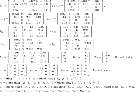
A11=

0 1 −0.266 −0.009 −2.75 −2.78 −1.36 −0.037

0 0 0 1

−4.95 0 −55.5 −0.039

, εA12=

0.0024 0 −0.087 0.002 −0.185 0 1.11 −0.011

0 0 0 0

0.222 0 8.17 0.004

,

εA13=

0.073 0 −0.25 0.003 −0.46 0 2.8 −0.02

0 0 0 0

0.924 0 17.5 0.02

, εA21=

0.021 0 0.121 0.003 −1.1 0 −1.62 −0.015

0 0 0 0

−2.43 0 1.37 −0.034

,

A22=

−0.21 1 −1.6 −0.005 −1.9 −1.8 9.3 −0.12

0 0 0 1

−3.1 0 −56 0.032

, εA23=

0.06 0 0.46 0.002 −1 0 1.49 −0.04

0 0 0 0

0.12 0 29.8 −0.028

,

εA31=

−0.002 0 0.83 0 −6.78 0 −10.1 0.09

0 0 0 0

−1.24 0 0.498 −0.017

, εA32=

0.011 0 0.22 0 −2.1 0 1.7 −0.123

0 0 0 0

−0.07 0 6.38 −0.011

,

A33=

−0.197 1 −1.2 −0.003 −54.5 −20 70.1 −2.37

0 0 0 1

−3.4 0 −21.0 −0.017

, B11=

0 36.1

0 0

, B22=

0 78.9

0 0

, B33=

0 1000 0 0

, Bij= 0, i=j,

E11=

0.1 0 0 0 0 0 0 0 0 0 0 0.1 0 0 0 0.1

, E22=

0 0 0 0 0.1 0 0 0 0 0 0 0.1 0 0 0 0.1

, E33=

0 0 0 0 0 0 0 0 0.1 0 0 0.1

0 0 0 0.1

, Eij= 0, i=j,

Vii=diag

1 2 2 1

, V1=block diag

Vii µ−1I4 µ−1I4

, V2=block diag

µ−1_I

4 Vii µ−1I4

, V3=block diag

µ−1_I

4 µ−1I4 Vii

, Q1=block diag

0.5I4 O8×8

, Q2=block diag

O4×4 0.5I4 O4×4

, Q3 =block diag

O8×8 0.5I4

, R11=R22=R33= 1, R12=R13= 0.2, R23=R21= 0.3, R31=R32= 0.1.

F₁(3)∗_ε =

−1.6070 −9.6942e−01 −7.2616 −2.0448e−02 −1.0183e−03 −8.1937e−06 −3.6317e−03 9.9899e−03 2.5572e−03 2.5593e−06 3.5754e−02 1.5000e−03 , F(3)∗

2ε =

−1.4029e−03 −3.3082e−05 2.9290e−02 1.4973e−03 −1.2967 −9.9375e−01 −7.9714 9.9917e−02 3.5550e−03 3.5495e−06 6.6756e−02 9.0373e−04 , F(3)∗

3ε =

−2.2157e−03 −5.8545e−05 −9.9676e−06 2.4311e−04 −1.1642e−03 −1.4511e−05 −5.4604e−03 8.6321e−04 1.5201 −9.8172e−01 −3.5409 3.0341e−01 .

The small parameters are chosen as_ε= 0_.01and_µ= 0_.005.

It is easy to verify that algorithm (11) converges to the exact solution with an accuracy of ||G(k)|| _< 1.0e − 11 after three iterations, where ||G(k)|| := ₃

i=1||Gi(P1(kε), P2(εk), P3(εk))||.

Table 1. Errors per iterations. k ||G(k)|| 0 1_.1923_e−01 1 6_.9726_e−04 2 3.1597e−08 3 3.1552e−11

In order to verify the exactitude of the solution, the remainder per iteration is substituted by _Piε(k) into CSAREs (6). In Table 1, the results of the error ||G(k)|| per iteration are given. As a result, it can be seen that algorithm (11) yields quadratic convergence.

Using the proposed design procedure, the high-order approximate soft-constrained Nash strategies (16) are

given by

u_i(3)∗(t) =F_iε(3)∗x(t), (42) where

F₁(3)_ε∗= ⎡ ⎣F011

0 ⎤ ⎦_{, F}(3)∗

2ε = ⎡ ⎣_F0₂₂

0 ⎤ ⎦_{, F}(3)∗

3ε = ⎡ ⎣ 00

F33

⎤ ⎦

and_Fii,_i= 1_, 2_, 3are given at the top of the next page. The costs using the high-order strategy (16) are com-puted. The initial conditions are chosen as _x(0) = [ 1 0 1 1 1 0 1 1 1 0 1 1 ]T. The cost functional-to-perturbation_ε2k+1ratio are given in Table 2, where

φi=| ¯

Jiapp−J¯iopt|

ε2k+1 , (43)

¯

Jiapp:= ¯Ji(u(1k)∗, ... , uN(k)∗, x(0)) =x(0)TYiεx(0), ¯

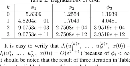
Table 2. Degradations of cost.

k φ1 φ2 φ3

0 5.8309 1.2554 1.1939

1 4_.8204_e−01 1_.7049 4_.0481 2 9_.0753_e+ 03 2_.7508_e+ 04 3_.9519_e+ 04 3 9_.0753_e+ 11 2_.7508_e+ 12 3_.9519_e+ 12

It is easy to verify that _J¯_i(_u1(k)∗_{, ... , u}(_Nk)∗_{, x}(0))− ¯

Ji(u∗1, ... , u∗N, x(0)) =O(ε2

k₊₁

) because of_φi<∞. It should be noted that the result of three iteration in Table 2 is not reliable because this result has the major error due to_O(_ε9)≈10−18.

VIII. CONCLUSION

In this paper, a higher-order approximate soft con-strained Nash strategy for weakly coupled large-scale systems has been proposed. Comparing with the existing result [5–8], there exist three useful and reliable con-tributions. First, the considered CSAREs have the sign-indefinite quadratic term. Thus, it succeeds in expanding the results for the general case. Second, in order to reduce the amount of the algebraic computation, the recursive algorithm was considered. This algorithm would result in reducing the CPU time. Third, by using these iterative so-lutions by means of the proposed two algorithm, the high-order approximate strategies have been proposed. As a result, it has been shown that the proposed strategy results in better performance. Finally, the numerical example has shown the excellent results.

REFERENCES

[1] W. A. V. D. Broek, J. C. Engwerda and J. M. Schumacher, “Robust Equilibria in Indefinite Linear-Quadratic Differen-tial Games,” J. Optimization Theory and Applications, vol. 119, no. 3, pp. 565-595, 2003.

[2] J.C. Engwerda, “A Numerical Algorithm to Find Soft-Constrained Nash Equilibria in Scalar LQ-Games,” Int. J.

Control, vol. 79, no. 6, pp. 592-603, 2006.

[3] J.D. Delacour, M. Darwish and J. Fantin, “Control Strate-gies for Large-Scale Power Systems,” Int. J. Control, vol. 27, no. 5, pp. 753-767, 1978.

[4] X. Shen, Q. Xia, M. Rao and V. Gourishankar, “Optimal Control for Large-Scale Systems : A Recursive Approach,”

Int. J. Systems Sciences, vol. 25, no. 12, pp. 2235-2244,

1994.

[5] H. Mukaidani, “Optimal Numerical Strategy for Nash Games of Weakly Coupled Large-Scale Systems,” Dyn.

Continuous, Discrete and Impulsive Systems, Series B: Applications and Algorithms, vol. 13, no. 2, pp. 249-268,

2006.

[6] H. Mukaidani, “A Numerical Analysis of the Nash Strategy for Weakly Coupled Large-Scale Systems,” IEEE Trans.

Automatic Control, vol. 51, no. 8, pp. 1371-1377, Aug.

2006.

[7] H. Mukaidani, “Newton’s Method for Solving Cross-Coupled Sign-Indefinite Algebraic Riccati Equations for Weakly Coupled Large-Scale Systems,” Applied

Mathe-matics and Computation, vol. 188, no. 1, pp. 103-115,

2007.

[8] H. Mukaidani, “High-Order Approximation of Soft Con-strained Nash Strategy for Weakly Coupled Large-Scale Systems,” in Proceedings of the 2007 IEEE International

Conference on Systems, Man, and Cybernetics, Montreal,

pp.145-150, October 2007.

[9] T. Yamamoto, “A Method for Finding Sharp Error Bounds for Newton’s Method under the Kantorovich Assump-tions,” Numerische Mathematik, vol. 49, no.2-3, pp. 203-220, 1986.

[10] B. Petrovic and Z. Gaji´c, “Recursive Solution of Linear Quadratic Nash Games for Weakly Interconnected Sys-tems,” J. Optimization Theory and Applications, vol. 56, no. 3, pp. 463-477, 1988.

[11] Z. Gaji´c, D. Petkovski and X. Shen, Singularly Perturbed

and Weakly Coupled Linear System - A Recursive Sp-proach. Lecture Notes in Control and Information

Sci-ences, vol.140, Springer-Verlag, Berlin; 1990.

[12] M. Lim and Z. Gaji´c, “Subsystem-Level Optimal Control of Weakly Coupled Linear Stochastic Systems Composed of N Subsystems,” Optimal Control Applications and

Methods, vol. 20, no. 20, pp. 93-112, 1999.

[13] X. Nian, S. Yang and N. Chen, “Guaranteed Cost Strategies of Uncertain LQ Closed-Loop Differential Games with Multiple Players,” in Proceedings of American Control

Conf., Minneapolis, pp. 1724-1729, June 2006.

[14] M. Jungers, A.L.D. Franco, E. De Pieri and H. Abou-Kandil, “Nash Strategy Applied to Active Magnetic Bear-ing Control,” in ProceedBear-ings of 16th IFAC world congress, Prague, CD-Rom, July 2005.

Muneomi Sagara received his B.S. degree in Education from

Hiroshima University, Japan, in 2005 and his master degree in Education form Hiroshima University, Japan, in 2007. He is currently Ph.D. candidate at Graduate School of Education, Hiroshima University. His current research interests include stochastic control systems and its application.

Hiroaki Mukaidani received his B.S. degree in integrated arts

and sciences from Hiroshima University, Japan, in 1992 and his M.Eng. and Dr.Eng. degrees in information engineering form Hiroshima University, Japan, in 1994 and 1997, respectively. He worked with Hiroshima City University as a Research Associate from 1998 to 2002. Since 2002, he has been with the Graduate School of Education, Hiroshima University, Japan, as an Assistant Professor and currently as an Associate Professor. His current research interests include robust control, dynamic game and its application of singularly perturbed systems and large-scale systems. He is a member of the Institute of Electrical and Electronics Engineers (IEEE).

Toru Yamamoto received his B.Eng. and M.Eng. degrees from