Dynamics of Macro–Nano Mechanical Systems;
Fixed Interfacial Multiscale Method
M. H. Korayem
*, S. Sadeghzadeh
Robotic Research Laboratory, Center of Excellence in Experimental Solid Mechanics and Dynamics,
School of Mechanical Engineering, Iran University of Science and Technology, Tehran, I. R. Iran
(*) Corresponding author: [email protected]
(Received:05 Sep. 2012 and Accepted: 20 Dec. 2012)
Abstract:
The continuum based approaches don’t provide the correct physics in atomic scales. On the other hand, the
molecular based approaches are limited by the length and simulated process time. As an attractive alternative,
this paper proposes the Fixed Interfacial Multiscale Method (FIMM) for computationally and mathematically efficient modeling of solid structures. The approach is applicable to multi-body mechanical systems. In FIMM, a direct link between the nano field atoms and macro field nodes by the local atomic volume displacements associated with every macro field node in their common zone has been replaced with the previous methods. For a complete model of the macro section, a nine-noded Lagrange element has been developed, and for small dimensions, the Sutton-Chen potential (for problems of mechanics) has been used. In the presented model, the undesirable effects of free surfaces, common surfaces, and surfaces close to the interface with the macro field
have been eliminated, and after presenting a practical and noteworthy procedure for the dynamics of systems
in general, seven problems (in the form of three examples) have been offered to showcase the practicality,
simplicity, and the effectiveness of this method.
Keywords: Multi-scale model; Open systems; Dynamics; Macro/nano mechanics; coupling model, FIMM.
Int. J. Nanosci. Nanotechnol., Vol. 8, No. 4, Dec. 2012, pp. 227-246
1. INTRODUCTION
Although they have been extensively applied for
simulation of large scales, the continuum
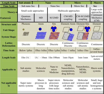
mechanics-based methods, including the finite element or other numerical methods, don’t provide the correct physics in atomic scales. Table 1 lists a complete span of various scales and models in material modeling. Upon the appearance of advanced technologies, the interfacial behavior of macro (large) to nano (small) scales has been discussed. Connectivity of models in various scales was the first and the best approach of course. This approach named Multiscale method and has been studied and developed in a lot of works for various systems. In multi-scale approaches, implementation of molecular based models guarantees the correctness of obtained behavior in small scales; while for larger dimensions that
don’t have tangible nonlinear behavior, utilization of continuum mechanics (CM) based methods is effective, and there is no need to spend a lot of time by application of the atomic models for these parts. Therefore, the continuum mechanics models and the atomic models interact with each other in such a way as to model the whole system and achieve the goal which has been defined and set.
228
microsecond dimensions is only possible by means
of supercomputers. So, researchers are trying to use
the advantages of the aforementioned methods and to overcome the existing flaws by combining them together. The outcome of these efforts has been the development of multi-scale methods.
Multi-scale methods are divided into “hierarchical” and “concurrent” groups. In the hierarchical models, the properties are calculated at one scale and then passed on to another scale. In other words, the information obtained from one model is enriched by another model. These approaches include two groups, in which, the information from micro-scale systems is transferred to the continuum mechanics model. The first group are the models based on the Cauchy-Born hypothesis [1, 2], in which, the information acquired from the atomic
structure of the object clearly reveal themselves in the calculation of the elastic stress and tensor of the material’s properties. The second group of these models is based on the Virtual Atom Cluster (VAC) [3], in which, the structure of the material is enriched on the basis of the information obtained from molecular mechanics. This method has been used for the study of carbon nano tubes.
In the concurrent models, there are several simultaneous models in the multi-scale simulation, and information is exchanged among them concurrently. These methods are the result of efforts that have tried to combine the molecular dynamics models with the continuum mechanics models. Over the past decade this group of multi-scale models has received considerable attention in the literature. It includes various frameworks, but
Korayem and Sadeghzadeh
Dynamics of Macro–Nano Mechanical Systems; Fixed Interfacial Multiscale Method
2- Introduction
Although they have been extensively applied for simulation of large scales, the
continuum mechanics based methods, including the finite element or other numerical
methods, don't provide the correct physics in atomic scales. Table 1 lists a complete
span of various scales and models in material modeling. Upon the appearance of
advanced technologies, the interfacial behavior of macro (large) to nano (small) scales
has been discussed. Connectivity of models in various scales was the first and the best
approach of course. This approach named Multiscale method and has been studied and
developed in a lot of works for various systems. In multi-scale approaches,
implementation of molecular based models guarantees the correctness of obtained
behavior in small scales; while for larger dimensions that don't have tangible nonlinear
behavior, utilization of continuum mechanics (CM) based methods is effective, and
there is no need to spend a lot of time by application of the atomic models for these
parts. Therefore, the continuum mechanics models and the atomic models interact with
each other in such a way as to model the whole system and achieve the goal which has
been defined and set.
Table 1. A complete span of various models in material modeling
Length Scale Sub atomic Nano Micro Macro
Time Scale Sub nano Sec Nano Sec Micro Sec Sec
Theory
Features
Small scale approaches Multiscale approaches Large scale approaches
Quantum
Mechanics MD SCGMD CM-MD coupling CM-SCGMD coupling
Continuum Mechanics
(CM)
Structure unit
Unit Shape
Phonons Atom Site Element-Atom Element-Site Element
System Shape
Lattice
Deformation Discrete Discrete Discrete Continuous-Discrete Continuous-Discrete Continuous
Time Scale Below 1pSec 1fSec-1nSec 1fSec-1μSec 1nSec- 1 mSec 1nSec-1Sec several hours
1mSec-Length Scale 1fm-1A� 1A� - 10nm 1fm-100nm 1nm-10μm 1nm-1mm 1μm-several meters
Applicable to Sub atomic studies Molecular sciences Nano to micro Medicine
NEMS, Nanorobotics, manipulation, drug delivery
Nanorobotics, MEMs,
NEMS
Macro scale systems
Not applicable
to metric systems Super nano
Macro processes in
long duration
Super micro processes with large time scales
Molecular sciences and
sub atomic studies
Molecular sciences and
sub atomic studies
Small, huge and non homogeneou
s systems
229
three major methods may be addressed. The quasi-continuum method [4, 5], which was presented by Ortiz et al., is now the most applied method, and many studies have been conducted on this method. The other model is the Bridging Domain method [6], which has been developed by Belytschko et al. In this method, in part of the simulation zone, the continuum domain and the atoms exist together; therefore, the validity of this model in the bridging domain needs to be investigated extensively. The third approach, known as the Bridging Scale method [7, 8], has been presented by Liu and his colleagues. In this method, it is assumed that the continuum solution is not exact and the resulting error can be removed through molecular dynamics. The most important issue in the development of these hybrid methods has been the formulation of a comprehensive computational coupling along the
interface.
This fact has been revealed in a brief review of the developed and presented methods. In the coupling models, the continuity of the material’s characteristics should be preserved during the
transition from the atomic forces to the
stress-strain field of continuum mechanics. Coupling models have been developed for many problems, including the crack problem, and they have often been named Finite Element–Atomistic (Feat) coupling procedure, which is the combination of molecular dynamics and finite element models. Likewise, a general formulation of the ordinary finite element, which allows the Macro Field (MF) nodes to be examined as coarse and fine Nano Field (NF) atoms, has resulted in another computational scheme for the coupling of the continuum and the atomic environments, called the Coarse-Grained Molecular Dynamic (CGMD).
The Quasi-Continuum (QC) method that has been studied by Miller and Tadmor [9] is explicitly based on the complete description of a material’s environment. The Coupled Atomistic/Dislocation Dynamics (CADD) method of Shilkrot et al. [10] has been presented for the simulation, detection, and justification of the separations between the atomic and the continuum regions. This model had first been offered for the simulation of materials at zero degrees Kelvin (0 K), but recently, it has been developed to deal with the effects of finite temperature as well.
The general characteristic of these approaches,
for the atomic and continuum coupling, has been the fine-graining and manipulation of MF mesh configuration for conformity with atomic length scales, and also the kinematic coupling of finite element nodes to discrete atoms along an interface.
Henceforth, the approaches that make a one to one
coupling between the atoms and finite element are called Direct Coupling (DC).
When DC procedures are followed, the major problem that arises is the inherent difference between the atomic and the continuum computational models. The physical state of the atomic region is described by means of the non-local inner-molecular forces between discrete atoms with specific position and moment; while the physical state of the continuum region is described by using the stress-strain fields which are statistical averages of the atomic attractions at larger scales of length and time. Generally, the ordinary coupling between discrete and continuum values can only be obtained by taking a statistical average of the scales in which the discreteness of the atomic structure can be approximated in the quasi-continuum form. Although, much better ways could be offered for the development of methods of coupling of the continuum domain with discrete domain, nevertheless, the application and development of these methods for the static and dynamic problems related to mechanical engineering is highly
important.
Up to now, the FEM was the most applied approach for macro part of coupling models; while, much better and more accurate methods, and even more exact numerical methods, exist for this purpose. Thus, in describing the problem, instead of the finite element method, the more general form of finite element, i.e. the MF solution method, is used. Based on this notion, we try to present a model that can be attached to the finite element method without any restriction, and can be used with other methods as well.
So far, various NF-MF coupling frameworks have been presented. The work of Park and Liu [11] is an attempt to describe the multiscale method ideas and capabilities in the field of solid structures. Recently, some concentrated groups have focused on the multiscale approaches for various applications. They introduced various frameworks with capabilities of application to solid structures. For instance, Macroscopic Atomistic
230
Ab initio Dynamics (MAAD) method [12, 13], Heterogeneous Multiscale Method (HMM) [14], Multiscale Field Theory (MFT) [15] and Embedded Statistical Coupling Method (ESCM) [16] may be addressed.
In this paper, a Fixed Interfacial Multiscale Method (FIMM) is proposed for computationally and mathematically efficient modeling of solid structures. The approach is applicable to multi-body mechanical systems. In FIMM, a direct link between the nano field atoms and macro field nodes by the local atomic volume displacements associated with every macro field node in their common zone has been replaced with the previous methods.
Moreover, considering the mechanics of the problem, and using a system of equations in matrix form, a dynamic algorithm has been presented for dynamically solving the problem. The macro and nano field’s computational systems are independent of each other and only relate through an iterative update of their boundary conditions. This method presents an improved coupling approach which is inherently applicable to three-dimensional domains. In addition, it prevents the resolving of the continuum model into atomic resolution, and allows finite temperature cases to be applied. One of the prominent features of the present work is
the presentation of reliable solutions for problems
that include natural, forced, body, and interfacial degrees of freedom. Since solids are fairly rigid at the macro zone, the interfacial volume of the considered system has been moved to macro part and then, it assumed to be rigid.
Thus, FIMM leaves negligible relative motion of atoms in every atomic volume by moving the interface into the macro part. Now, previous nano field and a bit of macro part form the new nano field. This leads to larger dimensions for nano field with regard to the last one. One major difference between ESCM and FIMM is the constraint of coupling, where ESCM uses a local average of atoms included in an interfacial volume.
In the following, both the macro (continuum model) and nano (atomistic model) field theories are discussed briefly first. Then, FIMM has been presented in details and validated by comparison with MD, CGMD, ESCM and MAAD approaches
for a clamped silicon wafer in plane strain condition. At the end several useful results and discussion have been introduced
2. AN OVERVIEW OF FEM AND MD
Extensive work has been done on the development of Finite Element Method for various systems. Since
in mechanical systems, usually the macro section
has a moving part and a sensing part, and these parts often operate by means of the piezoelectric property, we try to deal with the macro section from this perspective. Rajeev kumar et al. [17] investigated a finite element model for the active control of induced thermal vibration in layered composite shells with piezoelectric sensors and actuators (piezothermoelastic). Then, they presented a finite element formulation for the modeling of static and dynamic responses of multi-layered composite shells with integrated piezoelectric sensors and actuators, and subjected to mechanical, electrical, and thermal loadings [18].
In 2008, Zia et al. [19] have presented a finite element formulation for the vibrations of layered piezoceramic plates, which accounts for the effects of hysteretic behavior. The hysteretic behavior has been simulated in the dielectric domain by using the finite element method and applying the Ishlinskii’s model. In 2008, Balamurugan and Narayanan [20] have used a nine-noded piezolaminated degenerated shell element in order to model and analyze multi-layered composite shell structures together with sensors and piezoelectric actuators.
The coordinates of any arbitrary parameter, at any arbitrary point can be expressed by the use of nodal coordinates and isoparametric shape functions in the following way
1
( , , ) ( ) Q
i i
i X
ξ η ζ
==
∑
ℵP P (1)
Where
P
is the noted parameter,ℵ
is theisoparametric functions, Q is number of nodes of
the considered element, and X is the position of the
nodes. By using the kinetic, potential and external energies and writing the minimum energy principle, the equations of motion for the finite element system can be presented as:
Dynamics of Macro–Nano Mechanical Systems; Fixed Interfacial Multiscale Method
integrated piezoelectric sensors and actuators, and subjected to mechanical, electrical,
and thermal loadings [18].
In 2008, Zia et al. [19] have presented a finite element formulation for the vibrations of
layered piezoceramic plates, which accounts for the effects of hysteretic behavior. The
hysteretic behavior has been simulated in the dielectric domain by using the finite
element method and applying the Ishlinskii's model. In 2008, Balamurugan and
Narayanan [20] have used a nine-noded piezolaminated degenerated shell element in
order to model and analyze multi-layered composite shell structures together with
sensors and piezoelectric actuators.
The coordinates of any arbitrary parameter, at any arbitrary point can be expressed by
the use of nodal coordinates and isoparametric shape functions in the following way
1
( , , ) ( )
Q
i i
i
X
P P
(1)
Where
P
is the noted parameter,
is the isoparametric functions,
Q
is number of
nodes of the considered element, and
X
is the position of the nodes. By using the
kinetic, potential and external energies and writing the minimum energy principle, the
equations of motion for the finite element system can be presented as:
1 1e e e qe e
e e e e
M
uuq
C
uuq
K
uu
K K
u K
u
q
F
K K
u
F
(2)
where
Muu
e,
Kuu e,
K
u
e,
Fq e,
K
e,
Fe,
Cuu e, and
q
eare respectively, the
element's mass matrix, stiffness matrix, electromechanical coupling hardness matrix,
mechanical load, dielectric hardness matrix, electric force vector, structural damping
matrix, and the vector of change of degrees of freedom in the considered system.
In MD, a well defined potential function
U r r
1, , ,2 rN
expresses the manner of
dependency of the potential energy of a system consisting of N atoms with the space
coordinates
r r
1 2, , ,
r
N. The equation of motion of all atoms model can be expressed as
i i i i
m =-
r
U+F
(3)
Where, m and F are the mass of atoms and external (boundary) forces. The Finite
Difference Method (FDM) is the usual approach for solving the differential equations
of motion. FDM includes various approaches for analyzing the problem. Verlet and
Velocity Verlet algorithms are the most famous methods. These algorithms are
combination of the forward and backward Taylor expansions [21].
In addition to the Lenard Jones potential as a famous one, the Embedded Atom
Potential (EAM), Finnis-Sinclair potential [22] and Sutton-Chen potential [23, 24] may
be addresses as multi-particle potentials. They may be implemented in the simulation of
solid structures as well as the bio and fluidic fields. However, the solid structures are
231
where
[
Muu]
e,[ ]
Kuu e,
K
uφ
e, Fqe,
K
φφ
e,e
Fφ ,
[ ]
Cuu e, andq
eare respectively, the element’smass matrix, stiffness matrix, electromechanical coupling hardness matrix, mechanical load, dielectric hardness matrix, electric force vector, structural damping matrix, and the vector of change of degrees of freedom in the considered system. In MD, a well defined potential function
(
1, , ,2 N)
U r r … r expresses the manner of dependency of the potential energy of a system
consisting of N atoms with the space coordinates
1 2
, , ,
Nr r
…
r
. The equation of motion of all atomsmodel can be expressed as
Dynamics of Macro–Nano Mechanical Systems; Fixed Interfacial Multiscale Method
integrated piezoelectric sensors and actuators, and subjected to mechanical, electrical,
and thermal loadings [18].
In 2008, Zia et al. [19] have presented a finite element formulation for the vibrations of
layered piezoceramic plates, which accounts for the effects of hysteretic behavior. The
hysteretic behavior has been simulated in the dielectric domain by using the finite
element method and applying the Ishlinskii's model. In 2008, Balamurugan and
Narayanan [20] have used a nine-noded piezolaminated degenerated shell element in
order to model and analyze multi-layered composite shell structures together with
sensors and piezoelectric actuators.
The coordinates of any arbitrary parameter, at any arbitrary point can be expressed by
the use of nodal coordinates and isoparametric shape functions in the following way
1
( , , ) ( )
Q
i i
i X
P P
(1)
Where
P
is the noted parameter,
is the isoparametric functions,
Q
is number of
nodes of the considered element, and
X
is the position of the nodes. By using the
kinetic, potential and external energies and writing the minimum energy principle, the
equations of motion for the finite element system can be presented as:
1 1e e e qe e
e e e e
M
q
C
q
K
K K
K
q
F
K K
F
uu uu uu u u u
(2)
where
Muu
e,
Kuu e,
K
u
e,
Fq e,
K
e,
Fe,
Cuu e, and
q
eare respectively, the
element's mass matrix, stiffness matrix, electromechanical coupling hardness matrix,
mechanical load, dielectric hardness matrix, electric force vector, structural damping
matrix, and the vector of change of degrees of freedom in the considered system.
In MD, a well defined potential function
U r r
1, , ,2 rN
expresses the manner of
dependency of the potential energy of a system consisting of N atoms with the space
coordinates
r r
1 2, , ,
r
N. The equation of motion of all atoms model can be expressed as
i i i i
m =-
r
U+F
(3)
Where, m and F are the mass of atoms and external (boundary) forces. The Finite
Difference Method (FDM) is the usual approach for solving the differential equations
of motion. FDM includes various approaches for analyzing the problem. Verlet and
Velocity Verlet algorithms are the most famous methods. These algorithms are
combination of the forward and backward Taylor expansions [21].
In addition to the Lenard Jones potential as a famous one, the Embedded Atom
Potential (EAM), Finnis-Sinclair potential [22] and Sutton-Chen potential [23, 24] may
be addresses as multi-particle potentials. They may be implemented in the simulation of
solid structures as well as the bio and fluidic fields. However, the solid structures are
(3)
Where, m and F are the mass of atoms and external (boundary) forces. The Finite Difference Method (FDM) is the usual approach for solving the
differential equations of motion. FDM includes various approaches for analyzing the problem. Verlet and Velocity Verlet algorithms are the most famous methods. These algorithms are combination of the forward and backward Taylor expansions [21].
In addition to the Lenard Jones potential as a famous one, the Embedded Atom Potential (EAM), Finnis-Sinclair potential [22] and Sutton-Chen potential [23, 24] may be addresses as multi-particle potentials. They may be implemented in the simulation of solid structures as well as the bio and fluidic fields. However, the solid structures are especial nano fields that mentioned potential should be improved for better results. The Rafii-Tabar-Sutton multi-body long-range potential is used in the current study which is an extended and improved form of Sutton-Chen potential with the capability of modeling the unlike material’s interactions. The general form of Rafii-Tabar-Sutton (RTS) potential for binary A-B unlike materials is [23 , 24]:
Dynamics of Macro–Nano Mechanical Systems; Fixed Interfacial Multiscale Method
especial nano fields that mentioned potential should be improved for better results. The Rafii-Tabar-Sutton multi-body long-range potential is used in the current study which is an extended and improved form of Sutton-Chen potential with the capability of modeling the unlike material's interactions. The general form of Rafii-Tabar-Sutton (RTS) potential for binary A-B unlike materials is [23 , 24]:
RTS AA A BB B
I ij i i i i
i j¹i i i
1 ˆ ˆ
H = V r -d p ρ -d (1-p ) ρ
2
���With
AA
BB
AB
ij ˆ ˆi j ij ˆi ˆj ij ˆi ˆj ˆj ˆi ij
V r =p p V r + 1-p 1-p V r + p 1-p +p 1-p V r ���
A A AA AB
i ij j ij j ij
j i j i
ˆ ˆ
ρ = Φ r = pΦ r + 1-p Φ r
���
B B BB AB
i ij j ij j ij
j i j i
ˆ ˆ
ρ = Φ r = 1-p Φ r +pΦ r
���Where
p
ˆ
i is the site occupancy operator and defined as:i
1 if site i is occupied by an A atom
ˆp =
0 if site i is occupied by an B atom
���
The functions
V (r)
xy andΦ
xy(r)
are defined as
xy xyxy xy a n
V r =ε [ r ] ���
xy xyxy r =[a ]m
r
Φ ����
And the constants are defined by
AA AA AA
d =ε
C
d =ε
BB BB BBC
1 ( )
2
AB AA BB
m m m n = (n +n )AB 1 AA BB
2 ����
AB AA BB
a = a a εAB= ε εAA BB
Where
is a parameter with the dimensions of energy, 'a' is a parameter with the dimensions of length and is normally taken to be the equilibrium lattice constant, 'm' and 'n' are positive constants with n>m. This potential has the advantage that all the parameters can be easily obtained from the Sutton-Chen elemental parameters of metals232
Dynamics of Macro–Nano Mechanical Systems; Fixed Interfacial Multiscale Method
especial nano fields that mentioned potential should be improved for better results. The Rafii-Tabar-Sutton multi-body long-range potential is used in the current study which is an extended and improved form of Sutton-Chen potential with the capability of modeling the unlike material's interactions. The general form of Rafii-Tabar-Sutton (RTS) potential for binary A-B unlike materials is [23 , 24]:
RTS AA A BB B
I ij i i i i
i j¹i i i
1 ˆ ˆ
H = V r -d p ρ -d (1-p ) ρ
2
���With
AA
BB
AB
ij ˆ ˆi j ij ˆi ˆj ij ˆi ˆj ˆj ˆi ijV r =p p V r + 1-p 1-p V r + p 1-p +p 1-p V r ���
A A AA AB
i ij j ij j ij
j i j i
ˆ ˆ
ρ = Φ r = pΦ r + 1-p Φ r
���
B B BB AB
i ij j ij j ij
j i j i
ˆ ˆ
ρ = Φ r = 1-p Φ r +pΦ r
���Where pˆiis the site occupancy operator and defined as:
i
1 if site i is occupied by an A atom ˆp =
0 if site i is occupied by an B atom
���
The functions V (r)xy and Φxy(r)are defined as
xy xyxy xy a n
V r =ε [ r ] ���
xy xyxy r =[a ]m
r
Φ ����
And the constants are defined by
AA AA AA
d =ε C d =BB εBB BBC
1 ( )
2
AB AA BB
m m m n = (n +n )AB 1 AA BB
2 ����
AB AA BB
a = a a εAB= ε εAA BB
Where is a parameter with the dimensions of energy, 'a' is a parameter with the dimensions of length and is normally taken to be the equilibrium lattice constant, 'm' and 'n' are positive constants with n>m. This potential has the advantage that all the parameters can be easily obtained from the Sutton-Chen elemental parameters of metals [24].
(11)
Where
ε
is a parameter with the dimensions ofenergy, ‘a’ is a parameter with the dimensions of length and is normally taken to be the equilibrium lattice constant, ‘m’ and ‘n’ are positive constants with n>m. This potential has the advantage that all the parameters can be easily obtained from the Sutton-Chen elemental parameters of metals [24].
In a lot of existent mechanical systems, the small field includes a large area with respect to the atomic dimensions. For instance, in nanorobotic devices, the nano filed includes some nano and some micro parts. So, MD could not cover the simulation of nano field alone, yet MD may be modified to apply in larger sizes (with limitations in the aspect ratio). Clustering the all atom MD model into a coarse grained site model, named Coarse Grained MD (CGMD), is a simple and effective method for this
purpose.
3. COARSE-GRAINED MOLECULAR
DYNAMICS
Electromechanical processes normally occur on the order of nano, micro, milli, and even several seconds. In addition, they have higher-than-nano dimensions. Therefore, their real dimensions and time ranges cannot be determined through the use of molecular dynamics method. However, by the use of “coarse graining”, larger dimensions, in longer time ranges could be modeled.
Now, since a remarkable method by the name of Coarse-Grained Molecular Dynamics (CGMD) has been presented for this purpose, while using it here, a general description is also provided regarding this approach. The CGMD method is based on the notion that, if instead of one atom, a larger number of atoms are taken as a unit, then, a larger volume of material and also more simulation time can be considered. Even by utilizing the world’s largest
and most advanced supercomputers, the molecular dynamics simulations cannot be performed for more than several microseconds. Various approaches have been presented for the CGMD methods [21-23].
The only crucial issue in these models will be the manner of predicting and estimating the system’s potential. Achieving a good potential for the system can be guaranteed through a dimension analysis, and by comparing the Radial Distribution Function (RDF) of the system with obtained CGMD in the NF process; although, other ways also exist for this achievement. If, on the average, the nominal mass and distance of atoms are on the order of
'
m
c'
and' '
L
c , and the nominal mass and distanceof the CGNF samples are on the order of ‘m’and
‘L’, respectively, the following relations could be considered for the time steps that are used:
Dynamics of Macro–Nano Mechanical Systems; Fixed Interfacial Multiscale Method
In a lot of existent mechanical systems, the small field includes a large area with respected to the atomic dimensions. For instance, in nanorobotic devices, the nano filed includes some nano and some micro parts. So, MD could not cover the simulation of nano field alone, yet MD may be modified to apply in larger sizes (with limitations in the aspect ratio). Clustering the all atom MD model into a coarse grained site model, named Coarse Grained MD (CGMD), is a simple and effective method for this purpose.
4- Coarse-grained molecular dynamics
Electromechanical processes normally occur on the order of nano, micro, milli, and even several seconds. In addition, they have higher-than-nano dimensions. Therefore, their real dimensions and time ranges cannot be determined through the use of molecular dynamics method. However, by the use of "coarse graining", larger dimensions, in longer time ranges could be modeled. Now, since a remarkable method by the name of Coarse-Grained Molecular Dynamics (CGMD) has been presented for this purpose, while using it here, a general description is also provided regarding this approach. The CGMD method is based on the notion that, if instead of one atom, a larger number of atoms are taken as a unit, then, a larger volume of material and also more simulation time can be considered. Even by utilizing the world's largest and most advanced supercomputers, the molecular dynamics simulations cannot be performed for more than several microseconds. Various approaches have been presented for the CGMD methods [21-23]. The only crucial issue in these models will be the manner of predicting and estimating the system's potential. Achieving a good potential for the system can be guaranteed through a dimension analysis, and by comparing the Radial Distribution Function (RDF) of the system with obtained CGMD in the NF process; although, other ways also exist for this achievement. If, on the average, the nominal mass and distance of atoms are on the order of 'mc'and ' 'Lc , and the nominal mass
and distance of the CGNF samples are on the order of 'm' and 'L', respectively, the following relations could be considered for the time steps that are used:
max MD m
Δt ~L
kT and maxCGMD c c
m
Δt ~L
kT (12)
We developed a new CGMD approach and validated it with proper results [25]. It has been utilized in this paper for the NF.
5- Macro-micro coupling model
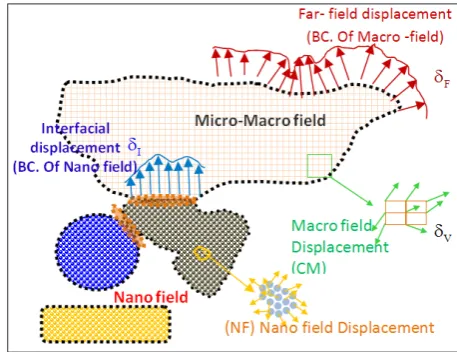
To generalize the problem, the macro-nano-related problems are divided into two groups of closed and open systems. The group of problems, where all the side boundaries of the nano domain overlap the interfacial degrees of freedom, are called "closed systems"; and the group of problems, where the side boundaries of the nano region, in addition to the interfacial degrees of freedom, possess limited (and in some cases, unlimited) degrees of freedom, are called "open systems". Figures 1 and 2 illustrate the general cases of the closed and open systems, respectively. In the closed
(12)
We developed a new CGMD approach and validated it with proper results [25, 26]. It has been utilized in
this paper for the NF.
4. MACRO-MICRO COUPLING MODEL
To generalize the problem, the macro-nano-related problems are divided into two groups of closed and open systems. The group of problems, where all the side boundaries of the nano domain overlap the interfacial degrees of freedom, are called “closed systems”; and the group of problems, where the side boundaries of the nano region, in addition to the interfacial degrees of freedom, possess limited (and in some cases, unlimited) degrees of freedom, are called “open systems”. Figures 1 and 2 illustrate the general cases of the closed and open systems, respectively. In the closed system, usually one nano field and one macro field exist. For example, in the crack propagation problem, the fine region of crack propagation is designated as the nano field, and the coarse region in which the crack is growing is designated as the macro field. In the open system, several macro fields could be interacting with several nano fields. If the numbers of macro and nano fields are equal to M and N, respectively, and
233
the area of each field is indicated by
Ω
, then for theclosed system, we can write:
, ,
, ,
, ,
i j
i j
i j
i j NF
or i j MF
i NF j MF
Ω ∩ Ω = ∅ ∈
Ω ∩ Ω = ∏ ∅ ∈
Ω ∩Ω ≠ ∅ ∈ ∈
(13)
And for the open system:
, ,
, ,
, ,
i j
i j
i j
or i j NF
or i j MF
or i NF j MF
Ω ∩ Ω = ∏ ∅ ∈
Ω ∩ Ω = ∏ ∅ ∈
Ω ∩Ω = ∏ ∅ ∈ ∈
(14)
In the above relations,
∅
and ∏denote theempty and non-empty spaces, respectively. With this notation, it can be easily proved (considering the presented definitions) that a closed system is a special case of an open system. Therefore, in an open system, there may be more than one nano field and each of the nano fields may be in contact with one another in different ways.
These contacts (for example in the nanomanipulation process using nanorobots) may not occur during a certain time range, and after that duration, these contacts may be established. Exclusively mechanical systems are taken into account, and therefore, the mentioned contacts are of the second order only, and volumetric sharing is not considered.
Figure 1: General case definition of closed
mechanical systems
Figure 2: General case definition of open
mechanical systems
The concept of multi-scale coupling methods can be very useful in cases where we want to model a relatively large region of the material in order to study the whole deformation field, but the atomic and sub-atomic scales are needed only in specific and limited regions. A practical example of a closed system can be demonstrated in the modeling of crack nucleation and propagation. As was mentioned before, for such problems, various works have been presented.
The present model has a special application in open systems; systems where practically no interface may even exist between the macro and nano environments in some cases and in a certain range of work, while after a certain time duration (which could be known or unknown), a relationship may form between these two environments. Through the use of coupling models for closed environments, the size limitation of atomic modeling could be minimized, such that an inner region (with complex dynamic processes and large deformation gradients) could exist inside an outer region (with small deformation gradients). It is not like this in open systems, where the effect of size will be considerable. To demonstrate the effectiveness of the model, in this article, the special case of a conic region for NF has been investigated. Also, in the MF model, an elastic beam with piezoelectric properties has been considered.
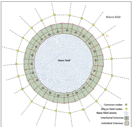
4.1. Coupling of MF and NF
For the coupling of MF and NF in closed
234
systems, four regions are considered throughout the system shown in Figure 3. These four regions, in the order of proceeding from micro to nano environments, consist of: Macro Field (MF), Unfolded Volume (UV), Interfacial Volume (IV), and Nano Field (NF). The IV region is in fact a region where the terminal atoms of a NF model have surrounded a MF node in the model. The IU region is the region between the end nodes of MF and the end of the NF model. The two regions of MF and NF need no further explanation. In view of the presented cases, IVs estimate the mean displacements of NF in the center of mass of these displacements. These averages are later used as the initial conditions of displacements in the relevant interfacial nodes. It should be mentioned that, the IV need not match the macro element that surrounds it, with respect to the size and shape.
Normally, a macro element, in the interfacial
section, consists of hundreds to thousands of atoms. By taking an effective average for the atomic points, the discreteness of the atomic structure can be sufficiently homogenized so that the MF region responds to the excitations of the atomic region as an expanded volume of itself.
Figure 3: Common region between NF and
MF in the closed system
For the analysis of open systems, in addition to the four regions of MF, UV, IV, and NF, two regions of Free Boundaries of nano field (denoted by FB)
Figure 4: Common region between NF and MF in the open system
235
and Common Boundaries of nano field (denoted by CB) are also defined (Figure 4). Regardless of the type of initial state these two regions may have, each one has the potential of undergoing different changes during the analysis time range. The CB region is usually circumscribed around a circular zone, because in small dimensions, for considering the forces which in this zone are accounted among different sections of the nano field, the concept of “cut off radius” is used. Moreover, the MF region is also divided into four sections of “free far-fields”, “internal volume”, “boundary field”, and “interfacial field”.
It seems necessary here to describe the method of analysis of the FB and CB regions. In order for the FB region to behave freely (at surface), changes should be made to the model. This is the philosophy behind the establishment of the FB region. The existence of free surface creates unwanted effects
in the NF system.
In comparison with the cases in which the boundary is affected by an external load, this occurrence in FB is not so critical. In addition to unwanted
effects, since atoms at the free surface or close to
it don’t have a complete set of neighboring atoms, the coordination between the atoms falls apart. To remedy this lack of coordination, and to make the atoms stable in the interfacial NF region, two approaches can be adopted. The first approach is to offer an additional volume of atoms away from the center, which forms the surface NF region. The second approach is to consider a number of the same NF system atoms as an unfolded volume. In case of using the first approach, although the
surface NF region eliminates the effects of the free
surface, it applies an unwanted virtual stiffness to the system, which elastically constrains the deformation of the inner NF region. To counteract this effect, the unwanted virtual hardness should be compensated. Since the effects of surface in solids are controllable, to a large extent, by the inner volume, in this article, it is suggested to use the second approach. Of course, in places where the limitation of size exists (like the tip of a cone-shaped region), the use of the first approach is inevitable. During the simulation, the average of k numbers of IV, for obtaining the displacement of the center of mass is defined as
δ
CM kMD,
, which, to get the statistical displacement vector
δ
I kMD,
, is averaged along M time ranges of NF:
(
)
, , , ,
1
1 M ( ) (0)
MD MD
I k CM k Time CM k j CM k j
r t r
M
δ
δ
=
= =
∑
−
(15)
In the above relation, ,
1
1
( )
Nk( )
CM k j i j
i k
r
t
r t
N
==
∑
is
center of mass of the kth IV, which has
k
N
atoms in the positionr
i
at time tjof the jth NF time range.
In open systems, in order for the NF region to behave freely (at surface) or to be subjected to specific external forces, some alterations should be made in the model. This is the philosophy behind the establishment of the UV region. In the best case, when the free movement of the surface is intended, the existence of the free surface produces unwanted
effects in the NF system.
This event, in cases where an external force is considered instead of the free movement, will be much worse. In addition to unwanted effects, since atoms at the free surface or close to it don’t have a complete set of neighboring atoms around them, the coordination between the atoms falls apart.
To reduce this lack of coordination, and to make
the atoms stable in the interfacial NF region, an
additional volume of atoms far from the center, which forms the surface NF region, is offered. On the other hand, although the surface NF region
eliminates the effects of the free surface, it applies
an unwanted virtual stiffness to the system, which elastically constrains the deformation of the inner NF region. Due to the particular complexity of the problem, in this report, a simple, and at the same time, effective procedure is presented for the calculation of virtual hardness.
4.2. Algorithm for establishment of coupling
In general, the coupling of MF and NF is accomplished through schemes based on the establishment of iterative equilibrium between these two regions. In these schemes, the iterations begin with the displacements of the MF and NF interface. These displacements are obtained as statistical average from the atomic positions of every IV, and by averaging in the time duration of NF. These average displacements are then applied in the MF
region, as displacement boundary conditions (
δ
I ).Then, the obtained MF boundary value problem is solved to yield the new interfacial reaction forces,