The mean-Value at Risk static portfolio optimization
using genetic algorithm
Vladimir Ranković1, Mikica Drenovak1, Boban Stojanović2
, Zoran Kalinić1 and Zora Arsovski1
1 Faculty of Economics, University of Kragujevac,
Djure Pucara 3, 34000 Kragujevac, Serbia [email protected] [email protected]
[email protected] [email protected]
2 Faculty of Science, Department of Mathematics and Informatics,
University of Kragujevac, Radoja Domanovica 12, 34000 Kragujevac, Serbia
Abstract. In this paper we solve the problem of static portfolio allocation based on historical Value at Risk (VaR) by using genetic algorithm (GA). VaR is a predominantly used measure of risk of extreme quantiles in modern finance. For estimation of historical static portfolio VaR, calculation of time series of portfolio returns is required. To avoid daily recalculations of proportion of capital invested in portfolio assets, we introduce a novel set of weight parameters based on proportion of shares. Optimal portfolio allocation in the VaR context is computationally very complex since VaR is not a coherent risk metric while number of local optima increases exponentially with the number of securities. We presented two different single-objective and a multiobjective technique for generating mean–VaR efficient frontiers. Results document good risk/reward characteristics of solution portfolios while there is a trade-off between the ability to control diversity of solutions and computation time.
Keywords: Genetic algorithm, Static portfolio optimization, Value at Risk, Mean-VaR efficient frontier.
1.
Introduction
solutions of Markowitz problem for different levels of return form the so-called efficient frontier which represents the optimal trade-off between the risk and return.
When using variance to estimate risk we implicitly assume that returns are normally distributed, i.e. that distribution is fully explained by first two moments, return and standard deviation. However, empirical distributions of returns typically are asymmetric distributions with more events in tails relative to normal distribution suggesting that part of the risk is hidden in the higher moments of distribution. The importance of third moment in portfolio optimization was first suggested by Samuelson [29] while Markowitz [26] suggested semivariance for the measure of downside risk.
Nowadays, investors and regulators are mostly concerned about the risk of extreme quantiles. The risk of extreme quantiles is typically measured by value at risk (VaR) and conditional value at risk (CVaR). Although it is not a coherent risk metric [30], VaR is a predominantly used risk measure of extreme quantiles, in particular upon the introduction of new banking regulations for market risk in 1996 [5].
By definition, VaR is the α-quantile of distribution. Unlike variance, VaR of a portfolio cannot be estimated analytically, as a function of underlying constituents’ parameters. Portfolio VaR can be estimated analytically, but only if we assume that portfolio data distribution (in value or return terms) can be accurately approximated by some theoretical distribution. In reality, especially during market turmoil, empirical return distributions of financial assets are typically asymmetric, with fat tail(s) and cannot be accurately approximated by any theoretical distribution.
Further, in Danielsson et al. [12], the authors demonstrated that the set of feasible portfolios under VaR constraint need not to be connected or convex, while the number of local optima increases exponentially with the number of securities.
In general, optimal portfolio allocation in the VaR context is very complex, often unsolvable by using classical optimization methods. In order to overcome drawbacks of classical optimization methods, several researchers applied metaheuristics (either single or multiobjective) for solving portfolio optimization problems.
The focus of this paper is on the effectiveness of different GA techniques for static portfolio optimization when return and percentage historical VaR are set as optimization objectives. We employed standard single-objective technique and SPEA2 method as a fully multiobjective technique to derive mean return-historical VaR efficient frontier. In addition, we introduced a novel single-objective GA technique, adjusted to specific characteristics of VaR measure. With the aim to improve execution efficiency, a novel set of weights which are constant over time for a static portfolio is introduced. We compared the differences between analyzed techniques and identified their relative advantages regarding risk/reward characteristics, diversity of solutions along efficient frontier and computational time.
2.
Related work
Depending on the applied risk model, portfolio optimization may be a highly nonlinear problem, very difficult to solve using deterministic methods. In practice, portfolio optimization problems become even more complex since they include a lot of additional constraints such as: cardinality constraints, transaction cost, trading limitation etc.
There have been various studies applying genetic algorithms for solving portfolio optimization problems based on different risk measures and/or additional constraints. One of the earliest attempts of GA portfolio optimization is given by Arnone, Loraschi, and Tettamanzi [4]. The authors considered bi-objective, mean return-risk, unconstrained portfolio optimization problem, regarding downside, variance based risk measures. They transformed bi-objective problem to a single-objective problem using trade-off coefficient. Lin and Liu [24] presented a study about portfolio optimization based on Markowitz model with the minimum transaction lots constraint. The authors generated mean-variance efficient frontiers by minimizing risk for given return levels using single-objective GA. Chang et al. [7] presented GA approach to mean return-risk portfolio optimization problems with the cardinality constraint. As in [4], the authors applied bi-objective to a single-objective problem transformation by using trade-off coefficient. As risk measures, the authors considered semi-variance, mean absolute deviation and variance with skewness. Branke et al. [6] considered mean-variance problem with maximum exposure constraint. The authors generated mean-variance efficient frontiers by using multiobjective evolutionary algorithms (MOEAs). Recently, Anagnostopoulos and Mamanis [3] presented an interesting study about effectiveness of five state-of-the-art MOEAs together with a steady state evolutionary algorithm on the mean–variance, cardinality constrained portfolio optimization problem. All enumerated papers examine Markowitz mean-variance model imposing different set of additional constraints.
Latest risk measurement practices trend toward quantifying and controlling risk of extreme quantiles, while VaR is a benchmark metric, as defined by regulators.
percentage historical VaR is used as a measure of risk. This is to the best of our knowledge the first attempt to do so in nonparametric VaR context by using GA approach.
3.
VaR model
VaR can be interpreted as a loss that will be exceeded only in α 100% of the time, for a given significance level α and time horizon t. Mathematically, VaR is defined as α-quantile of distribution. Expressed in value terms, VaR is the α-quantile of profit and loss distribution, while expressed as a percentage of portfolio’s value it is the α-quantile of return distribution.
Formally, for the return r such that p r
r
percentage VaR is defined as:VaR r . (1)
where α is significance level (i.e. 1-α is confidence level) and F-1(α) denotes α-quantile
of return distribution r, that is, the inverse of distribution function at α. Minus sign is needed since VaR is defined as positive value. If the distribution function of returns,
F(α), is known then α-quantile is calculated as 1
r F.When empirical
distribution of portfolio returns is used VaR is referred to as historical VaR.
Historical VaR does not assume any parametric form of the distribution of risk factor returns (see [28] for more details on historical VaR and its variants). It is rather intuitive and easy to calculate measure at portfolio level. On the other hand, when using historical VaR there is potential risk to underestimate risk of future movements since historical VaR assumes that realized distribution would be repeated in the future. In addition, historical VaR estimates are dependent on a sample size and may result in conflicting results for different significance levels. Yet, Perignon and Smith [27] report that almost 75% of banks prefer to use historical VaR rather than alternative VaR models.
In general, historical VaR cannot be expressed as a function of underlying constituents’ parameters. Thus, to perform portfolio optimization in VaR context, calculation of time series of portfolio returns is required. If using the definition Eq. (1), the estimate of historical VaR equals minus value of maximum of the subset containing α percentage of the lowest returns of considered portfolio (e.g. for time series consisted of 100 returns, 5% historical VaR would be minus value of 5-th lowest return).
4.
Decision variables
By definition, percentage one-period portfolio return rpat time t is:
, 1
1 t p t
t
P r
P
where Pt denotes total value of portfolio at time t:
, 1
N t i i t
i
P n p
. (3)
N is total number of assets, niis the number of shares of asset i and pi,t is the price per share of asset i at time t.
In [1] it is shown that percentage one-period portfolio return can be expressed as weighted sum of the asset returns:
, , 1 ,
1
N p t i t i t
i
r w r
. (4)
where ri,t denotes percentage one-period return of asset i at time t, while wi,t denotes proportion of capital invested in asset i at time t, given as:
,
, , 1,...,
i i t i t
t
n p
w i N
P
. (5)
Expression (4) is fundamental relationship in portfolio mathematics [1].
For static (buy-and-hold) portfolio, which is the focus of the paper, number of shares ni remains the same for each asset i over the observed period. Consequently, the proportion of capital invested in each asset wi,t changes over time, whenever the price of any asset in portfolio changes. In typical portfolio optimization methods, starting with those applying Markowitz model, static portfolio is considered, while portfolio weights are defined as a proportion of capital invested (Eq. (5)) in each portfolio constituent. Basic assumption is that portfolio weights are constant over time. Assumption of constant weights implies frequent portfolio rebalancing which further implies transaction costs that affect overall portfolio performance.
The main drawback of using wi,t weight parameters for calculating time series of “real” static portfolio returns is the fact that it requires recalculations of their values for every time interval during an observation period (e.g. for daily time series of portfolio returns daily recalculations of wi,tweights are needed).
In order to overcome this drawback we introduce different set of weights wi. Here i
w is defined as the proportion of shares held in asset i:
i i T n w N
. (6)
and 1 N T i i N n .
It can be seen that wiweights are properly defined since their values lie between 0 and 1 for long-only portfolios (that is, for portfolios without short positions) and they sum up to 1.
,
, 1 ,
1 1
,
, 1 , 1 , 1
1 1 1
1 1 1
N
N i N
i t
i i t i i i t
i T i
p t N N N
i
i i t i t i i t
i i i
T
n p
n p N w p
r
n
n p p w p
N
. (7)
Weights wi for static portfolio are, by definition, constant over observation period. Using Eq.(5) and Eq. (6), proportion of capital wi,t, which is of interest for an investor, is given as:
, ,
,
, ,
1 1
i T i t i i t
i t N N
i T i t i i t
i i
w N p w p w
w N p w p
. (8)
In the portfolio optimization problem, presented in this paper, weights wiare adopted as decision variables.
5.
Optimization model
Using definition of VaR (Eq. (1)),the portfolio optimization problem can be defined as follows:
min VaR( )w r . (9)
, 1 max T p t t p r r T w . (10)
1
1 N
i i
subject to w
. (11)
0wi1, i1,...,N . (12)
where
w denotes the vector of weights wi, VaR(w) denotes the value at risk of a portfolio, rp
w is the expected return of portfolio and T denotes the time series length. Eq. (9) minimizes VaR of the portfolio. Eq. (10) maximizes the expected return of portfolio. Eq. (11) describes the standard budget constraint which requires that proportions (weights) must sum up to 1.Eq. (12) describes the constraint that no short sales are allowed, which means that none of the weights can be negative.
deteriorating in terms of the other one. Each efficient portfolio represents a point in the objective functions space. Hence, the set of efficient portfolios represents a curve in the return-risk space connecting the portfolio with maximum return and portfolio with minimum risk. Often, this curve is called the efficient frontier. The aim of the portfolio optimization presented by the model is to find portfolios along the efficient frontier.
The presented optimization problem is the bi-objective optimization problem and can be solved using two different approaches.
The first technique implies transformation of bi-objective problem to single-objective problem using trade-off coefficient λ ( 0 1). The result is single-objective fitness function instead of two separate single-objective functions. In that case optimization problem (Eq. (9), Eq. (10)) becomes:
max f rp w 1 VaR w . (13)
In Eq. (13) the case λ = 1 corresponds to portfolio with maximum expected return and λ = 0 corresponds to portfolio with minimum VaR (risk). Values of λ satisfying 0 <
λ < 1 correspond to the portfolios lying on the efficient frontier.
The advantage of presented approach is that a single-objective technique can be used. The additional advantage is that decision maker (investor) can predefine the importance of each objective. This approach is known as decision before search approach [20], [21].
The main drawback of this approach is that each value of coefficient λ produces only one efficient portfolio, i.e. only one point of the efficient frontier. Therefore, if efficient frontier is needed, the set of separate calculations with different λ is required, which can be very time consuming.
The second approach implies use of fully multiobjective techniques. In this paper, results obtained using the both approaches are presented.
6.
Genetic Algorithms
The term evolutionary algorithms (EA) or evolutionary strategies, addresses a class of stochastic optimization methods which emulate the natural evolution. The origins of EAs can be found in the late 1950s, and since the 1970s several evolutionary methodologies have been proposed. This class of optimization methods addresses genetic algorithms, evolutionary programming, and evolution strategies [10].
In order to solve the portfolio optimization problems defined in previous sections, genetic algorithm is used.
Genetic algorithm is a stochastic optimization technique invented by Holland based on the Darwin principle that in the nature only “the fittest survive” [19]. The main idea of Holland’s theory is the application of the basic phenomena of the biological evolution such as inheritance, crossover and mutation, in order to find (generate) a solution that fits best. In the case of the portfolio optimization problems, term “the fittest” corresponds to the optimal portfolio.
usually referred to as chromosomes. Each chromosome, i.e. candidate solution, represents a decision vector made of decision variables. In the vocabulary of genetic algorithms each decision variable in the chromosome is called a gene.
In this research, each individual (chromosome) presents one weight vector w. Therefore, each gene corresponds to weight wi defined by expression (6)
Generally, genetic algorithm consists of the following steps: 1. Initialization of population with random individuals,
Initial population with the stated dimension of randomly chosen individuals is generated with the aim to uniformly cover the solution space.
2. Fitness evaluation of the individuals in the population,
Fitness value is assigned to each individual from the population defined by adopted fitness function.
3. Generation of a new population, using crossover and mutation,
Population of offspring is generated by applying crossover and mutation operators to population of parents.
4. Selection of individuals according to their fitness using some strategy (e.g. a Roulette wheel selection),
The aim of the selection process is to provide a set of offspring which “survived” and will be transmitted to the next generation.
5. Stop if terminating condition is satisfied (e.g., a fixed number of iterations), otherwise go to step 2.
In the following text the basic operators of genetic algorithm developed in this research are presented.
6.1. Initialization
First step of genetic algorithm is initialization of population. It is very important since initial population is supposed to cover the solution space in a best possible way. The second demand is to provide random and independent generation of individuals in order to ensure independence of each single run of GA. Therefore, each gene (weight parameter) within the individual has to be generated randomly and independently. At the same time, each individual constraint, defined by Eq. (12), must be satisfied.
In order to realize independence and randomness of gene generation the following procedure is used:
For each individual I in the population P:
1. Generate vector o that contains randomly chosen indexes of weights in vector w:
int
1, , 1, 2,...,o i rand N i N
where N denotes the number of assets held in portfolio; randint() is random function with uniform distribution of integers within the range [1,N]. Vector o defines the order of genes’ initialization.
1
1 1
1
0,1 1 , 1,..., 1
1
i real
o i o j
j N
o N o j
j
w rand w i N
w w
. (14)
where randreal() denotes random function with uniform distribution of real numbers within the range [0,1].
6.2. Crossover
In this research a basic (simple) crossover operator is implemented. The basic crossover operator involves two parents and produces two offspring (two new individuals). Idea is to divide both parents’ chromosomes in two segments at dividing point (gene) and then to swap obtained segments. Operator is stochastic one, because the dividing point is chosen randomly each time operator is applied. Usually, newborn offspring does not satisfy constraint defined by Eq. (12) and hence additional normalization of offspring is required.
6.3. Mutation
The mutation operator is implemented as follows. First, a set of randomly chosen individuals that will mutate is generated. For each individual from this set two genes are randomly selected. Then, the value of the first gene (weight parameter) is increased by some predefined value (e.g. 0.1) and the value of the second gene is decreased by the same value. In order to ensure satisfaction of constraint defined by Eq. (12) the following principle is applied. If new gene (weight) value is <0 then it is set to be =0. Also, if the new gene value is >1 it is set to be =1. For both cases, normalization of chromosome must be applied.
6.4. Selection
The aim of selection process is to choose the individuals from the current population who will survive. According to the analogy with living beings, the individuals that fit best will survive and be transmitted to the next generation. The fitness of each individual is determined by using of adequate fitness function. The strategy which implies that only the best fitted individuals survive is known as Elitistic strategy. Generally, using this strategy, search algorithm would relatively quickly find the optimized solution. The major drawback of this approach is tendency to get stuck on a local extremum.
transferred to the next generation. In this way, the best individual (solution) obtained during the evolution process is kept. The rest of generation is processed throughout
Roulette wheel selection.
Roulette wheel selection is partly stochastic strategy which is commonly used in GA approaches to portfolio optimization problems (see for example [22], [31]). Selection process is random but based on fitness value of individuals. If an individual is with better fitness value it has more chance of being selected and vice versa.
In order to apply Roulette wheel selection, relative fitness is introduced. Relative fitness of each individual is defined as
, min, 1,...,
r k k
f f f k M . (15)
where fk is fitness value of k-th individual, fminis minimal fitness value obtained in the current generation and M is population size.
Using the relative fitness value, a fictive “roulette wheel” can be constructed. Each
field of the fictive roulette wheel corresponds to one individual and the width of each field is proportional to relative fitness of that individual. The width of each roulette wheel field can be defined as range:
1
, ,
1 1
1 ,1
, , 2,...,
0,
k k
k r i r i
i i
r
rwf f f k M
rwf f
. (16)
Now, k-th individual in the population will be selected if following expression is satisfied:
,
1
0,M r i k
i
rand f rwf
. (17)
where randreal() is random function with uniform distribution of real numbers within the defined range.
7.
Data and research results
Underlying indices for sample ETFs are debt portfolios with exposure to euro zone sovereign debt. First 7 ETFs comprise representative sample of debt portfolios which target bonds from 5 to 10 years maturity segment1 while the latter 3 ETFs target
overall bond indices which include different maturity segments.
In times of market turmoil investors typically move towards less risky and more liquid financial products, such is sovereign debt. At the same time, current financial crisis strongly affected euro zone sovereign debt due to increased credit and liquidity risk concerns. Yield spreads rose sharply while correlations dropped. As a consequence, empirical return distributions of sovereign debt portfolios are more often characterized by extreme events. Investing in sovereign debt of euro zone countries through ETFs is arguably the most liquid way of getting desired exposure during the crisis while daily data are publicly available.2 The motivation for choosing 5-10
maturity segment ETFs for the research is the fact that their return distributions are highly non-normal for chosen sample period (see more on characteristics of euro zone sovereign debt ETFs in [15] and [16]).
We compare risk/return characteristic of optimized portfolios to those of individual assets and to the 1/n portfolio. DeMiquel et al. [14] evaluated the out-of-sample performance of Markowitz model of optimal asset allocation and its various extensions (in total 14 different models). The authors demonstrated that naïve optimization rule 1/n of assets in portfolio is good proxy of optimal portfolio and can be challenged against more sophisticated portfolio designs. We employed static version of 1/n portfolio in order to be consistent with our basic assumption that all portfolios are buy-and-hold portfolios.
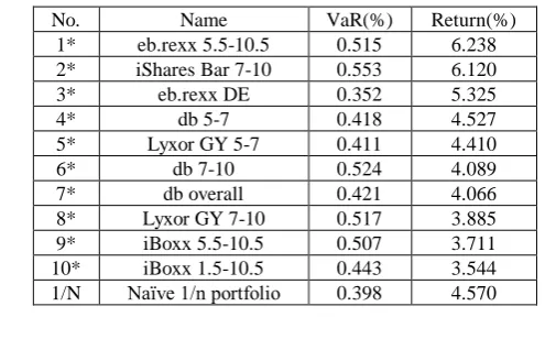
Table 1 shows 1-day historical VaR and average 1-day annualized return values for sample ETFs and naïve 1/n portfolio.
Table 1. 5% 1-day historical VaR and average 1-day annualized return values for sample ETFs and naïve 1/n portfolio
No. Name VaR(%) Return(%)
1* eb.rexx 5.5-10.5 0.515 6.238
2* iShares Bar 7-10 0.553 6.120
3* eb.rexx DE 0.352 5.325
4* db 5-7 0.418 4.527
5* Lyxor GY 5-7 0.411 4.410
6* db 7-10 0.524 4.089
7* db overall 0.421 4.066
8* Lyxor GY 7-10 0.517 3.885
9* iBoxx 5.5-10.5 0.507 3.711
10* iBoxx 1.5-10.5 0.443 3.544
1/N Naïve 1/n portfolio 0.398 4.570
1 These are all European ETFs targeting 5-10 year maturity segment of euro zone sovereign debt
with available time series of data long enough for this research.
2 Sovereign debt markets are typically over-the-counter markets where data are not publicly
Genetic algorithm, described in the previous sections, is coded in C# and run on personal computer with Intel Core(TM)2 Duo CPU E7300 2.66GHz processor and 2GB of RAM.
For solving optimization problem Eq. (9)-(12) three different techniques are applied (denoted as A1, A2 and A3, respectively). Therefore, results refer to three different sets of optimized portfolios, that is, on three different efficient frontiers.
Techniques A1 and A2 are based on the transformation of bi-objective optimization problem into single-objective problem using trade-off coefficient λ (Eq. (13)). In the A1 technique we examined equidistant values of trade-off coefficient λ. Within A2 technique we applied strategy of searching for optimized portfolios with predefined levels of return. For single-objective techniques we used following parameters: initial population size equals 200, number of generations equals 500 per single run, crossover rate equals 0.9, mutation rate equals 0.1.
Technique A3 employs fully multiobjective optimization genetic algorithm, the SPEA2 method (Strength Pareto Evolutionary Algorithm 2).
7.1. Single-objective technique A1 - Equidistant values of trade-off parameter
In this section we present the results of solving portfolio optimization problem for transformed VaR model (Eq. (13)) using 21 equidistant values of trade-off parameter λ within the range [0,1].
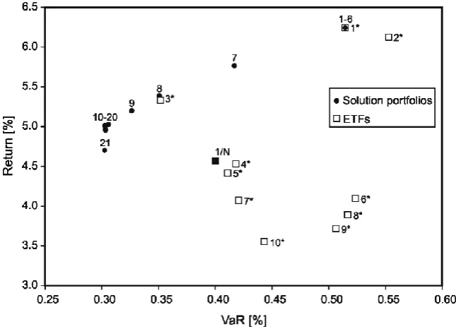
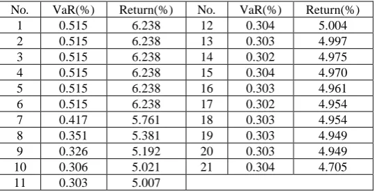
Optimized portfolios are plotted in return and risk (VaR) coordinates are presented with filled dots (Fig. 1). Single asset values are presented with squared dots. Each filled dot in the following graph is obtained by execution of genetic algorithm using one single value of parameter λ. Different values of parameter λ correspondto different relative importance of merged objective functions (return and risk). Efficient frontier is generated by repeating optimization procedure for each predefined value of λ. Optimized portfolios are numerated in decreasing order by return. 5% 1-day historical VaR and average 1-day annualized return values for optimized portfolios are presented in the Table 2. Asterisk numeration corresponds to sample ETFs presented in Table 1.
Table 2. 5% 1-day historical VaR and average 1-day annualized return values for optimized portfolios obtained using single-objective technique A1
No. VaR(%) Return(%) No. VaR(%) Return(%)
1 0.515 6.238 12 0.304 5.004
2 0.515 6.238 13 0.303 4.997
3 0.515 6.238 14 0.302 4.975
4 0.515 6.238 15 0.304 4.970
5 0.515 6.238 16 0.303 4.961
6 0.515 6.238 17 0.302 4.954
7 0.417 5.761 18 0.303 4.954
8 0.351 5.381 19 0.303 4.949
9 0.326 5.192 20 0.303 4.949
10 0.306 5.021 21 0.304 4.705
11 0.303 5.007
It can be seen from Fig. 1 that A1 technique results in portfolios with superior risk/reward characteristics compared to the individual assets from the sample and to the naïve 1/n portfolio. The results motivate the need for portfolio diversification and bring some evidence about the effectiveness of chosen algorithm. However, the plots presented in the graph show that equidistant values of trade-off parameter do not provide uniform distribution of solution portfolios along the resulting efficient frontier. It should be emphasized that diversity of points along the efficient frontier is crucial in portfolio optimization. Higher level of diversity implies more alternative portfolios, suited for the investors with different risk-return profiles.
7.2. Single-objective technique A2 - Imposing return levels
max min min
min 0 max 1
, 0,1,.., 20 20
,
p p
i p
p p p p
r r
l r i i
r r r r
. (18)
where lidenotes i-th return level.
For each return level an optimization process is executed. Each execution represents bisection iterative method implemented to determine λ corresponding to the considered return level. Finally, each iteration of the bisection method implies one single run of genetic algorithm which results in one solution portfolio.
Since it is impossible to reach the exact value of requested return level, for each execution of bisection iterative method we applied the following stop criterion:
max min
1 , , 0.1
20
2 30
p p
n
p i i
r r
r l tol l tol tol
or n
. (19)
where n denotes number of iterations, n p
r denotes return of the portfolio obtained in n-th iteration.
In the Fig. 2 we present mean-VaR efficient frontier for sample ETFs obtained using A2 technique. Corresponding 5% 1-day historical VaR and average 1-day annualized return values for optimized portfolios are presented in the Table 3.
Table 3. 5% 1-day historical VaR and average 1-day annualized return values for optimized portfolios obtained using single-objective technique A2
No. VaR(%) Return(%) No. VaR(%) Return(%)
1 0.515 6.238 12 0.353 5.392
2 0.497 6.165 13 0.343 5.314
3 0.483 6.086 14 0.332 5.245
4 0.471 6.002 15 0.324 5.162
5 0.458 5.929 16 0.320 5.091
6 0.442 5.854 17 0.305 5.012
7 0.423 5.778 18 0.303 4.962
8 0.408 5.704 19 0.300 4.862
9 0.400 5.622 20 0.301 4.788
10 0.382 5.543 21 0.304 4.705
11 0.364 5.465
Fig. 2 shows that A2 technique results in portfolios that are better distributed along the efficient frontier compared to solutions computed by A1 technique. Also, it should be noticed that for all, except for one predefined return level, proposed iterative procedure reached portfolio with return within targeted range.
Since VaR is not a coherent risk metric, it is very important to emphasize that solution portfolios obtained by single-objective techniques are not necessarily efficient portfolios in terms of given definition. It can be noticed from Fig. 2 that the solution portfolios corresponding to the two lowest return levels are not efficient portfolios since they are dominated. These points are not excluded in order to demonstrate the specificity of VaR.
7.3. Multiobjective technique A3 - SPEA2 method
In this section, we present the results obtained using multiobjective evolutionary algorithm (MOEA). Several different MOEA techniques can be found in the modern literature such as: Strength Pareto evolutionary algorithm 2 (SPEA2) [32], nondominated sorting genetic algorithm II (NSGA-II) [13], Pareto envelope-based evolutionary algorithm (PESA) [8], Niched Pareto genetic algorithm 2 (NPGA2) [9], e-multiobjective evolutionary algorithm (e-MOEA) [17].
In this research, we applied Strength Pareto evolutionary algorithm 2 (SPEA2). For more details see [32].
Common to all MOEAs techniques is the performance of full multiobjective optimization without transformation of multiobjective problem into single-objective.
Therefore, the input optimization problem for SPEA2 method is defined by Eq. (9)-(12).
Fig. 3. Mean-VaR efficient frontier for sample ETFs-A3 technique
Table 4. 5% 1-day historical VaR and average 1-day annualized return values for optimized portfolios obtained using multiobjective technique A3 (portfolios are numerated in decreasing order by return, M stands for multiobjective technique)
No. VaR(%) Return(%) No. VaR(%) Return(%)
1M 0.503 6.092 21M 0.404 5.625
2M 0.498 6.080 22M 0.395 5.591
3M 0.497 6.047 23M 0.390 5.541
4M 0.492 6.021 24M 0.386 5.433
5M 0.484 6.020 25M 0.384 5.427
6M 0.483 5.982 26M 0.382 5.416
7M 0.480 5.944 27M 0.379 5.407
8M 0.461 5.929 28M 0.369 5.382
9M 0.457 5.856 29M 0.367 5.351
10M 0.453 5.841 30M 0.364 5.323
11M 0.446 5.824 31M 0.355 5.281
12M 0.444 5.823 32M 0.347 5.260
13M 0.440 5.799 33M 0.337 5.208
14M 0.430 5.763 34M 0.336 5.163
15M 0.428 5.758 35M 0.334 5.142
16M 0.421 5.747 36M 0.327 5.139
17M 0.420 5.744 37M 0.310 5.020
18M 0.419 5.711 38M 0.310 4.976
19M 0.416 5.664 39M 0.308 4.956
Fig. 3 shows mean-VaR efficient frontier for sample ETFs obtained using SPEA2 method (no filled dots). In order to compare A2 and A3 techniques we keep the results presented in the Fig. 2 (A2 efficient frontier and sample ETFs). A3 optimized portfolios are not numerated in the figure for clarity reasons, but 5% 1-day VaR and average 1-day annualized return values are given in the Table 4.
Fig. 3 shows that A3 technique results in portfolios that are well distributed along efficient frontier. At the same time solution portfolios are slightly dominated by solution portfolios computed by A2 technique. Opposing the A2 technique, efficient frontier provided by A3 technique, lacks solution portfolios around maximum return, as well as, around minimum risk.
8.
Concluding remarks
In this paper we presented different GA techniques for the optimization of static portfolios in the context of historical VaR. In general, historical VaR cannot be expressed as a function of underlying constituents’ parameters. Thus, to perform portfolio optimization in VaR context, calculation of time series of portfolio returns is required. If considering static (buy-and-hold) portfolio, commonly used portfolio weights, given as proportion of capital invested in individual assets, are function of time. Therefore, when applying these weights to calculate daily time series of returns, one needs daily recalculations of weights. In order to avoid daily recalculations, for decision variables we adopted alternative portfolio weights which are based on proportion of shares of individual assets. For static portfolios, proposed weights are constant during the sample period. We showed that commonly used weights can be easily expressed as a function of the weights that we adopted.
In general, optimal portfolio allocation in the VaR context is computationally very complex and, very often, alternatives to existing exact optimization methods are required. In order to generate mean-VaR efficient frontier we used genetic algorithm. We tested two single-objective GA techniques and one multiobjective technique.
We first applied single-objective technique which uses the set of equidistant trade-off parameter values. It is clear from Fig. 1 that solution portfolios trade-offer much better risk/reward characteristics compared to individual assets from our sample. However, results also showed that chosen set of trade-off parameter does not provide uniform distribution of portfolios along the resulting efficient frontier. The second shortfall of this technique is that it is time consuming. Namely, for each value of trade-off parameter single run of genetic algorithm is needed. Execution time of single genetic algorithm was approximately 15 seconds. Hence, for portfolio optimization with 21 different values of trade-off parameter total execution time was approximately 5 minutes.
levels. As a result, we achieved the same level of diversification as was the case for the former technique, and, at the same time, returns of solution portfolios are well distributed along efficient frontier and satisfy predefined return levels. However, adding bisection method in the optimization algorithm further increased time needed for determination of each solution portfolio. In this research approximately 25 iterations of bisection method were needed. Therefore, execution time of second technique is on average 25 times longer than execution time of first technique. In particular, for portfolio optimization with 21 predefined levels of portfolio return execution time was approximately 125 min.
We emphasize that, formally speaking, single-objective techniques applied to VaR based portfolio optimization do not necessarily result in a set of efficient portfolios. The reason is that VaR is not a coherent risk measure while single-objective techniques are based on a sequence of independent executions.
As an alternative to single-objective approach we applied multiobjective evolutionary algorithm – SPEA2 method. Results show that solution portfolios are well distributed along efficient frontier, but it should be noticed that solution portfolios are slightly dominated by solution portfolios computed by A2 technique. On the other hand, when using multiobjective evolutionary algorithm we are not able to impose return levels of solution portfolios. The main advantage of SPEA2 method is computation time which in this research was approximately 3 minutes.
From an investor’s point of view, eligible portfolio optimization technique should provide her with:
1. efficient portfolios with returns distributed within the given range,
2. possibility to obtain portfolio with minimum risk for desired level of return, 3. acceptable computation time.
We showed that presented single-objective technique with imposed return levels (A2) satisfy conditions 1 and 2, while multiobjective technique (A3) satisfies conditions 1 and 3.
Financial implications of presented results would be of interest for all those investors who employ historical analysis for portfolio structuring, which is imposed by constraints in the context of VaR measure. In this respect, out-of-sample performance analysis of VaR optimized portfolios would be an interesting topic for further research.
Acknowledgement. Research presented in this paper was supported by Serbian Ministry of Science and Technology, Grants III-44010 and OH 179005.
References
1. Alexander C.: Quantitative Methods in Finance (1th ed.), John Wiley & Sons Ltd,
(Chapter 1). England. (2008).
2. Alexander C.: Value-at-Risk Models (1th ed.), John Wiley & Sons Ltd, (Preface).
England. (2008).
3. Anagnostopoulos, K.P., Mamanis, G.: The mean-variance cardinality portfolio
4. Arnone, S., Loraschi, A., Tettamanzi, A.: A genetic approach to portfolio selection. Neural Network World, Vol. 6, 597–604. (1993)
5. Basel Committee on Banking Supervision: Amendment to the capital accord to incorporate
market risks. (1996). [Online]. Available: http://www.bis.org. (current October 2013).
6. Branke J., Scheckenbach B., Stein M., Deb K., Schmeck H.: Portfolio optimization with
an envelope-based multi-objective evolutionary algorithm. European Journal of Operational Research, Vol. 199, 684–693. (2009)
7. Chang, T.-J., Yang, S.-C., Chang, K.-J.: Portfolio optimization problems in different
measures using genetic algorithm. Expert Systems with Applications, Vol. 36, 10529– 10537. (2009).
8. Corne, D. W., Knowles, J. D., Oates, M. J.: The Pareto envelope-based selection
algorithm for multi-objective optimization. In Proceedings of the parallel problem solving from nature (PPSN VI), Lecture notes of computer science, Vol. 1917, 839–848. (2000).
9. Erikson, M., Mayer, A., Horn, J.: The niched Pareto genetic algorithm 2 applied to the
design of groundwater remediation systems. In Zitzler, E., Thiele, L., Deb, K., Coello, C.A.C., Corne D. (eds.): Lecture notes in computer science, Vol. 1917, 681–695. (2001).
10. Cox, E.: Fuzzy Modeling and Genetic Algorithms for Data Mining and Exploration (1th
ed.), Morgan Caufmann, San Francisco, USA. (Chapter 9). (2005).
11. Dallagnol, V. A. F., Van den Berg, J., Mous, L.: Portfolio Management Using Value at
Risk: A Comparison between Genetic Algorithms and Particle Swarm Optimization. International Journal of Intelligent Systems, Vol. 24, 766–792. (2009).
12. Danielsson, J., Jorgensen B. Casper G., Yang X.: Optimal Portfolio Allocation Under the
Probabilistic VaR Constraint and Incentives for Financial Innovation. (2007). [Online]
Available: http://www.riskresearch.org/files/BJ-CdV-JD-01-8-11-997520309-11.pdf.
(current October 2013).
13. Deb, K., Ptratap, A., Agarwal, S., Meyarivan, T.: A fast and elitist multiobjective genetic
algorithm: NSGA II. IEEE Transactions on Evolutionary Computation, Vol. 6, 182–197. (2002).
14. DeMiguel, V., Garlappi, L., Uppal, R.: Optimal Versus Naive Diversification: How
Inefficient is the 1/N Portfolio Strategy? Rev. Financ. Stud., Vol. 22(5), 1915-1953. (2009).
15. Drenovak, M, Urosevic, B.: Exchange-traded funds of the Euro zone sovereign debt,
Economic Annals, Vol. 187, 31-60. (2010).
16. Drenovak, M., Urosević, B., Jelic, R.: European bond ETFs – tracking errors and the
sovereign debt crisis, European Financial Management. (2012).
[Online] Available:
http://onlinelibrary.wiley.com/doi/10.1111/j.1468-036X.2012.00649.x/abstract. (current October 2013).
17. Hanne, T.: A multiobjective evolutionary algorithm for approximating the efficient set.
European Journal of Operational Research, Vol. 176, 1723–1734. (2007).
18. Hoklie; Zuhal, L.R.: Resolving multi objective stock portfolio optimization problem using
genetic algorithm. In Proceedings of the 2nd International Conference on Computer and Automation Engineering (ICCAE). IEEE Conference Publications, Singapore, Vol. 2, 40-44, (2010)
19. Holland, J. H.: Adaptation in natural and artificial systems: An introductory analysis with
applications to biology, control, and artificial intelligence. University of Michigan Press. (1975).
20. Horn, J.: Multicriteria decision making. In B¨ack, T., Fogel, D. B., Michalewicz, Z. (eds.):
Handbook of Evolutionary Computation. Inst. of Physics Publ, Bristol, UK: (pp F1.9:1-F1.9:15). (1997).
21. Hwang, C.-L., Masud, A. S. M.: Multiple Objectives Decision Making—Methods and
22. Jiah-Shing, C., Jia-Li, H., Shih-Min, W., Ya-Wen, C.C.: Constructing investment strategy portfolios by combination genetic algorithms. Expert Systems with Applications, Vol. 36, 3824-3828. (2009).
23. Lin, P. C., Ko, P.C.: Portfolio value-at-risk forecasting with GA-based extreme value
theory, Expert Systems with Applications, Vol. 36, 2503–2512. (2009).
24. Lin, C. C., Liu, Y. T.: Genetic algorithms for portfolio selection problems with minimum
transaction lots. European Journal of Operational Research, Vol. 185, 393–404. (2008).
25. Markowitz, H. M.: Portfolio selection. Journal of Finance, Vol. 7, 77–91. (1952).
26. Markowitz, H. M.: Portfolio Selection: efficient diversification of investments. New York:
John Wiley & Sons, (Chapter 9). (1959).
27. Perignon, C., Smith, D.: The Level and Quality of Value-at-Risk Disclosure by
Commercial Banks, Working paper. (2006). [Online] Available:
http://www.unifr.ch/controlling/seminar/2007-2008/Perignon_ParisII.pdf, (current October 2013).
28. Pritsker, M.: The hidden dangers of historical simulation. Journal of Banking & Finance,
Vol. 30, 561-582. (2006).
29. Samuelson, P.: The fundamental approximation theorem of portfolio analysis in terms of
means variances and higher moments. Review of Economic Studies, Vol. 25, 65–86. (1958).
30. Szego, G.: Measures of risk. Journal of Banking & Finance, Vol. 26, 1253–1272. (2002).
31. Xiaolou, Y.: Improving Portfolio Efficiency: A Genetic Algorithm Approach.
Computational Economics, Vol. 28, 1-14. (2006).
32. Zitzler, E., Laumanns, M., Thiele, L.: SPEA2: Improving the strength Pareto evolutionary
algorithm, TIK-103. Zurich, Switzerland: Department of Electrical Engineering, Swiss Federal Institute of Technology. (2001).
Vladimir Ranković, PhD, Associate professor, University of Kragujevac, Faculty of Economics, Department for Statistics and Informatics, Serbia. He received his PhD degree in Computer modeling and simulations at the University of Kragujevac. Dr. Vladimir Rankovic has been involved in several national and international scientific projects related to computer modeling and simulations, numerical methods and software development. His current research focuses on intelligent systems and computational methods and techniques in economics and finance. This includes evolutionary multi-objective optimization techniques and theirs application in portfolio optimization and supply chain optimization and management.
Mikica Drenovak, PhD, Assistant professor, University of Kragujevac, Faculty of Economics, Department for Statistics and Informatics, Serbia. He received his Masters degree in Quantitative Finance and PhD in Finance from Faculty of Economics, University of Belgrade. His research interests include Financial Markets, Financial Regulation, Asset and Risk Management and Credit Derivatives.
hydroinformatics. He is author and co-author of one monograph and more than ten publications in peer reviewed journals and a number of simulation software. He has participated in several international scientific projects, FP7 and TEMPUS projects, and is prime investigator in bioengineering project with Northeastern University, Boston.
Zoran Kalinić, PhD, Assistant professor, University of Kragujevac, Faculty of Economics, Department for Statistics and Informatics, Serbia. He received his Ph.D. degree in Mobile Information Systems Design at the Faculty of Engineering, University of Kragujevac in 2012. Zoran Kalinic has been involved in several research projects related to information systems and software design. Also, he has taught as a guest lecturer at Cracow University of Economics, Poland. He is author/co-author of more than 50 scientific papers and monograph chapters. His current research interests include e-business, the application of artificial intelligence techniques in economics and finance, mobile communications and information systems and supply chain management.
Zora Arsovski, PhD, Full professor, University of Kragujevac, Faculty of Economics, Department for Statistics and Informatics, Serbia. Her current research interest includes information systems, software engineering, CIM systems, e-business, supply chain management, business process management, decision support systems, expert systems and business intelligence. Author and co-author on nine books and monographs, several chapters in scientific monographs, and more 220 articles published in international and national journals and conferences. She is a member of Editorial and Scientific board for several international journals and conferences. Also, she has taught as a guest lecturer at Cracow University of Economics, Poland. She was participated in seven international projects, nine national scientific projects, and realized more 40 projects of information systems on different ICT platforms.