29
A Variational-Fixed Point Iterative technique for the
Solution of Second Order Differential Equations
1
Adem Kilicman,
2K.R Adeboye,
1*Mutah Wadai
1Institute for Mathematical Research, Universiti Putra Malaysia *
Corresponding Author: [email protected]
2 Department of Mathematics, Federal University of Technology Minna, Nigeria
ABSTRACT In this paper, we propose a variational-fixed point iteration technique for the solution of second order linear differential equations with two-point boundary value problems. The proposed method is endowed with the Galerkin method for the determination of the starting function. The numerical results show the validity and efficiency of the proposed method in comparison withthe exact solution and other existing methods.
(Keywords: Variational iteration method, Galerkin method, Fixed point iteration method, Differential equation)
INTRODUCTION
In the rapid development and growth of the sciences, problems mostly occur as linear and nonlinear differential equations. Many scientists are involved in the attempt to come out with methods with better approximations to the solutions of the given problems that are close to analytic solution (Araghi F. M. A., 2011). Many methods have been developed and others are still being developed. Some of these developed methods have their own limitations which have to undergo changes either to shed more light on their behavior or improve on their accuracy (Araghi F. M. A., 2011; He J. H., 2012; Kilicman A.,Wadai M., 2016). Few, among many methods developed, are the variational iteration method, the fixed point iteration method and so on. These methods have been proved by many authors to be one of the mathematical tools for solving linear and nonlinear differential equations (Araghi F. M. A., 2011; Lu J., 2007). Researchers have shown that the variational iteration method is flexible with good convergence property (He J. H.,2000). However, the success of the method depends on the careful choice of the starting function which is usually done by guessing (Daniel T., et al., 2012; Wu G. C., 2013; Kilicman A.,Wadai M., 2016; Lu J., 2007. In this study, we propose a Variational-Fixed Point Iterative technique where the starting function is determined by the use of the Galerkin approximation. The presentation of this article is as follows: In Section 2 we present the methodology, Section 3 deals with the numerical results and finally discussion and conclusion are given in the last section.
METHODOLOGY
The variational iteration method can be illustrated by considering differential equation LU +NU = g(s), where L and N are linear and nonlinear operator respectively while g(s) is a forcing term. According to variational iteration method, a correctional functional can be constructed as follows:
𝑡𝑛+1(𝑥) = 𝑡𝑛(𝑥) + λ ∫ (𝐿𝑈0𝑥 𝑛(𝑠) + 𝑁𝑈𝑛(𝑠) − 𝑔(𝑠))𝑑𝑠 [1] where λ is a Lagrange multiplier, which can be identified optimally via variational theory, (He J. H., 2000; He J. H., 2007; Lu J., 2007; Noor M. A. & Mohyuddin S.T., 2008), the subscripts denotes the nth
iteration (He J.H., 2008; He J.H., 2006), un is
considered as a restricted variation. i.e dUn= 0, also a
simple formula has been developed where λ can easily be identified as
𝜆 =(𝑚−1)!(−1)𝑚(𝑡 − 𝑥)𝑚−1 [2]
to achieve convergence of result (Wu G. C., 2013). In order to overcome the difficulty of choosing the starting function 𝑡𝑛(𝑥) at n = 0 we employ the use of Galerkin method so as to have better choice of initial value to enhance convergence, which is illustrated as follows:
𝑈(𝑥) = 𝑈𝑜(𝑥) + 𝐶1𝑈1(𝑥) + 𝐶2𝑈2(𝑥) + ⋯ +
𝐶𝑛𝑈𝑛(𝑥) [3]
which is called the basis function where C1,C2, . . . ,Cn
30
process (Gerald F. C., 2004). After single iteration of variational iteration method we obtain 𝑡1(𝑥) which becomes the starting value of the fixed point iterative method; it is simple and easy to manipulate so that the process will be repeated until convergence occurs or the iteration is terminated, and thus
𝑦𝑛+1(𝑥) = (1 −∝𝑛)𝑦𝑛+∝𝑛𝑇𝑦𝑛 𝑦′
𝑛+1(𝑥) = (1 −∝𝑛)𝑦′𝑛+∝𝑛𝑇𝑦′𝑛 ⋮
𝑦′′
𝑛+1(𝑥) = (1 −∝𝑛)𝑦′′𝑛+∝𝑛𝑇𝑦′′𝑛.
NUMERICAL EXPERIMENTS
Three experiments are considered to demonstrate our method.
Experiment 1. Consider
𝑦′′− 𝑦 = −2𝑥2 ,0 ≤ 𝑥 ≤ 1 [4] subject to the boundary conditions
𝑦(0) = 0, 𝑦(1) = 6. [5] The analytic solution is given by
𝑦𝐸(𝑥) = 0.626070571𝑒𝑥− 0.626070571𝑒−𝑥+ 2𝑥2+ 4. [6] We apply the Galerkin Method to solve the problem. Let
𝑈(𝑥) = 6𝑥 + 𝐶1(𝑥 − 𝑥2) + 𝐶2(𝑥 − 𝑥3). [7]
After differentiating eq (7) twice and then substitute in eq (4) we get
−2𝐶1− 6𝐶2(𝑥) − 6𝑥 − 𝐶1(𝑥 − 𝑥2) + 𝐶2(𝑥 − 𝑥3) = −2𝑥2 [8] Let
𝑅(𝑥, 𝐶1, 𝐶2) = −2𝐶1− 6𝐶2(𝑥) − 6𝑥 − 𝐶1(𝑥 − 𝑥2) + 𝐶2(𝑥 − 𝑥3) + 2𝑥2 [9]
be the residual. Then apply the Galerkin processes as follow
∫(𝑥 − 𝑥2)(𝑅(𝑥, 𝐶 1, 𝐶2) 1
0
) = 0
∫(𝑥 − 𝑥3)(𝑅(𝑥, 𝐶 1, 𝐶2) 1
0
) = 0.
Then solving both integral equations to obtain
𝐶1= −47354, 𝐶2= −2843 . [10] Substitute eq(10) into eq(7) to get
𝑈(𝑥) = (2476473) 𝑥 + (47354) 𝑥2+ (28 43) 𝑥
3. [11]
By evaluating eq(11) at x = 0.5 we obtain
𝑈(0.5) = 2.727272727 . [12]
Now we will apply Variational Iteration Method as follows. Let us construct correctional functional
𝑡𝑛+1(𝑥) = 𝑡𝑛(𝑥) + 𝜆 ∫ (𝑡′′0𝑥 𝑛(𝑠) − 𝑡𝑛(𝑠) + 2𝑥2 (𝑠))𝑑𝑠 [13] Let us assume our initial guess
𝑡0 = 𝐴𝑥 + 𝐵. [14]
We differentiate eq (14) twice and substitute into eq(13) at n =0, 𝜆 = (s − x) to get
𝑡1(𝑥) = 𝐴𝑥 + 𝐵 −2(−(𝐴𝑥+𝐵)+2𝑥1 2 )𝑥2 [15]
By imposing the boundary conditions in eq(15), we obtain A = 14/3,B = 0. Substitute these values back in eq(15) to get
𝑡1(𝑥) = (143) 𝑥 −2(−(14 1 3)𝑥+2𝑥2)𝑥2
[16]
Then we evaluate eq(16) where x = 0.5 to get
𝑡1(0.5) = 2.562500000. [17]
Now we apply the variational-fixed point iteration technique as follows, that is, we use the Galerkin method as our starting values. Let
𝑈(𝑥) = 6𝑥 + 𝐶1(𝑥 − 𝑥2) + 𝐶2(𝑥 − 𝑥3) [18]
where C1 and C2 are constants to be determine using the
Galerkin Method. After differentiating eq(18) twice and then substitute into eq(4) we get
𝐶1= −47354 , 𝐶2= −2843 [19] Then substitute eq(19) into eq(18) to get
𝑈(𝑥) = (2476473) 𝑥 + (47354) 𝑥2+ (28 43) 𝑥
3 [20]
We now apply the variational iteration method using eq (20 ) as a starting value which we will then eventually obtain
𝑡1(𝑥) = (2476473) 𝑥 + (47354) 𝑥2+ (2843) 𝑥3−12(108473− (628473) 𝑥 + (892473) 𝑥2− (28
43) 𝑥
3) [21]
then we evaluate eq(21) at x = 0.5 to get
𝑡1(0.5) = 2.732954545. [22]
We then apply the new method by using t1(x) as
starting value as follows. Let
31
At n = 0 we have
𝑦′′
1(𝑥) = 𝑦0(𝑥) − 2𝑥2 [24] where
𝑦0(𝑥) = 𝑡1(𝑥) [25]
Substitute eq (25) into eq (24) to get
𝑦′′
1(𝑥) = ( 2476
473) 𝑥 + ( 54
473) 𝑥2+ ( 28 43) 𝑥3 − ((1
2)( 108 473− (
628 473) 𝑥 + (
892 473) 𝑥2 − (28
43) 𝑥3)𝑥2
[26] We integrate eq(26) twice successively to get
𝑦1(𝑥) = ( 1238
1419) 𝑥3− ( 1
6) 𝑥4+ ( 311 4730) 𝑥5
+ 1/129)𝑥7− (223/7095)𝑥6+ 𝐶 1𝑥 + 𝐶2
[27] imposing the boundary conditions for eq(27) we obtain
𝑦1(𝑥) = ( 1238
1419) 𝑥3− ( 1
6) 𝑥4+ ( 311 4730) 𝑥5 + (1/129)𝑥7− (223/7095)𝑥6 + (37264/7095)𝑥
[28] we repeat the process successively up to 7th iteration to
obtain
𝑦7(𝑥) = (1/3113535308083200)𝑥19− (63090057558528000233 ) 𝑥18+ ( 311
14020012790784000) 𝑥 17−
(52306974720001 ) 𝑥16+ ( 619
154632494016000) 𝑥 15−
(217945728001 ) 𝑥14+(2329/2761294536000)𝑥13− (1197504001 ) 𝑥12+(1341499/10195549056000)𝑥11− (9072001 ) 𝑥10+ ( 880361
60825718800) 𝑥
9− ( 1 10080) 𝑥
8+
(662710688640069060513719 ) 𝑥7− ( 1 180) 𝑥
6+ (10151896102421 231948741024000) 𝑥
5−
(16) 𝑥4+ (2510287020960113 2867729889024000) 𝑥
3(2360924944683800977 449516660104512000) 𝑥
[29] then we evaluate 𝑦7at x = 0.5 to get
𝑦7(0.5) = 2.726362232 [30]
Experiment 2. Consider the problem
𝑦′′− 𝑦 = −2𝑥; 0 ≤ 𝑥 ≤ 1 [31] subject to the boundary conditions
𝑦(0) = 0, 𝑦(1) = 3. [32]
The analytic solution is given by
𝑦𝐸(𝑥) =𝑒
1(𝑒𝑥−𝑒−𝑥)
𝑒2−1 + 2𝑥. [33]
We apply the Galerkin method to solve the problem. Let
𝑈(𝑥) = 3𝑥 + 𝐶1(𝑥 − 𝑥2) + 𝐶2(𝑥 − 𝑥3) [34]
after differentiating eq(34) twice and then substitute in eq (31) we get
−2𝐶1− 6𝐶2(𝑥) − 3𝑥 − 𝐶1(𝑥 − 𝑥2) − 𝐶2(𝑥 − 𝑥3) = −2𝑥 [35] and let
𝑅(𝑥, 𝐶1, 𝐶2=) = −2𝐶1− 6𝐶2(𝑥) − 𝑥 − 𝐶1(𝑥 − 𝑥2) − 𝐶2(𝑥 − 𝑥3) [36]
be the residual. Then by applying Galerkin processes as follow
∫(𝑥 − 𝑥2)(𝑅(𝑥, 𝐶 1, 𝐶2) 1
0
) = 0
∫(𝑥 − 𝑥3)(𝑅(𝑥, 𝐶 1, 𝐶2) 1
0
) = 0.
Then solving both integral equations to obtain
𝐶1=4738 , 𝐶2= −437 [37] Substitute eq(37) into eq(34) to get
𝑈(𝑥) = (1350473) 𝑥 − (8/473)𝑥 + (7/43)𝑥3. [38]
Then we evaluate eq(38) at x = 0.5 to get
𝑈(0.5) = 1.443181818. [39]
Now we will apply Variational Iteration Method as follows.
Let us construct correctional functional
𝑡𝑛+1(𝑥) = 𝑡𝑛(𝑥) + 𝜆 ∫ (𝑡′′0𝑥 𝑛(𝑠) − 𝑡𝑛(𝑠) +
2𝑥(𝑠))𝑑𝑠. [40]
Let assume our initial guess
𝑡0(𝑥) = 𝐴𝑥 + 𝐵 [41] we differentiate eq(41) twice and substitute to eq (40) when n = 0, 𝜆 = (s − x) to get
𝑡1(𝑥) = 𝐴𝑥 + 𝐵 − 1/2(−(𝐴𝑥 + 𝐵) + 2𝑥)𝑥2 [42]
32
𝑡1(𝑥) = (83) 𝑥 + (13) 𝑥3. [43]Then we evaluate eq(43) where x = 0.5 to get
𝑡1(0.5) = 1.375000000. [44]
Now we apply the variational fixed point iteration method as follows. We use the Galerkin method as our starting values instead of guessing as follows. Let
𝑈(𝑥) = 3𝑥 + 𝐶1(𝑥 − 𝑥2) + 𝐶2(𝑥 − 𝑥3) [45]
where C1 and C2 are constants to be determine using
Galerkin Method. After differentiating eq (45) twice and then substitute in eq(31) we get
𝐶1=4738 , 𝐶2= −437 . [46]
Substitute eq(46) into eq(45) to get
𝑈(𝑥) = (1350473) 𝑥 − (8/473)𝑥 + (7/43)𝑥3 [47]
We now apply the variational iteration method using eq(43)as a starting value we eventually obtain
𝑡1(𝑥) = ( 1350
473) 𝑥 − (8/473)𝑥 + (7/43)𝑥3 − (1/2(− 16
473+ ( 58 473) 𝑥 + ( 8
473) 𝑥2− ( 7
43) 𝑥3)𝑥2
[48] We evaluate eq(48) at x = 0.5 to get
𝑡1(0.5) = 1.441761363. [49]
We then apply the new method by using t1(x) as
starting value as follows. Let
𝑦′′𝑛+1=𝑦𝑛(𝑥) − 2𝑥, 𝑛 = 0,1,2, … [50] At n = 0 we have
𝑦′′𝑛+1=𝑦0(𝑥) − 2𝑥 [51] where
𝑦0(𝑥) = 𝑡1(𝑥). [52] Substitute eq(52) into eq(51) to get
𝑡1(𝑥) = (404473) 𝑥 − (8/473)𝑥 + (7/43)𝑥3−
( 1
2(−47316+(47358)𝑥+(4738 )𝑥2−(7 43)𝑥3)𝑥2
[53]
We integrate eq(53) twice successively to get
𝑦1(𝑥) = (1419202) 𝑥3+ (236512 ) 𝑥5+ (5161 ) 𝑥7− (70952 ) 𝑥6+ 𝐶
1𝑥 + 𝐶2 [54]
And imposing the boundary conditions for eq(54) we obtain
𝑦1(𝑥) = (1419202) 𝑥3+ (236512 ) 𝑥5+ (5161 ) 𝑥7− (70952 ) 𝑥6+ (80909
28380) 𝑥 [55]
We repeat the process successively up to 3rd iteration to
obtain
𝑦3(𝑥) = (371521 ) 𝑥9− (1986601 ) 𝑥8+ (165552 ) 𝑥7+ (14190101 ) 𝑥5+ (24149
170280) 𝑥 3+
(8155639/
2860704)𝑥 [56]
Then we evaluate y3 at x = 0.5 to get
𝑦3(0.5) = 1.443410956 [57]
Experiment 3. Consider the problem
𝑦′′− 𝑦′= −4𝑥 ; 0 ≤ 𝑥 ≤ 1 [58] subjects to the boundary conditions
𝑦(0) = 0, 𝑦(1) = 3. [59] The analytic solution is given by
𝑦𝐸(𝑥) = 1.745930121 − 1.745930121𝑒𝑥+ 4𝑥 + 2𝑥2. [60] We apply the Galerkin method to solve the problem. Let
𝑈(𝑥) = 3𝑥 + 𝐶1(𝑥 − 𝑥2) + 𝐶2(𝑥 − 𝑥3). [61]
After differentiating eq(61) twice and substituting into eq(58) we get
−2𝐶1− 6𝐶2𝑥 − 3 − 𝐶1(1 − 2𝑥) − 𝐶2(1 − 3𝑥2) = −4𝑥 [62]
Let
𝑅(𝑥, 𝐶1, 𝐶2) = −2𝐶1− 6𝐶2(𝑥) − 3 − 𝐶1(1 − 2𝑥) − 𝐶2(1 − 3𝑥2) + 4𝑥 [63]
be the residual. Then by applying the Galerkin processes as follow
∫(𝑥 − 𝑥2)(𝑅(𝑥, 𝐶 1, 𝐶2) 1
0
= 0
∫(𝑥 − 𝑥3)(𝑅(𝑥, 𝐶 1, 𝐶2) 1
0
33
and solving both integral equations, we obtain
𝐶1= −7761, 𝐶2=3061 . [64]
Substitute eq(64) into eq(61) to get
𝑈(𝑥) = (13661) 𝑥 − (7761) 𝑥2+ (30 61) 𝑥
3 [65]
Then evaluate eq(65) at x = 0.5 to get
𝑈(0.5) = 1.368852458 [66]
Now, we apply the Variational Iteration Method as follows. We construct the correctional functional as
𝑡𝑛+1(𝑥) = 𝑡𝑛(𝑥) + 𝜆 ∫ (𝑡′′0𝑥 𝑛(𝑠) − 𝑡′𝑛(𝑠) +
2𝑥(𝑠))𝑑𝑠. [67] Assume our initial guess to be
𝑡0(𝑥) = 𝐴𝑥 + 𝐵 [68]
By differentiating eq(68) twice and substituting into eq(67) atn = 0, 𝜆 = (s − x) we get
𝑡1(𝑥) = 𝐴𝑥 + 𝐵 − (12) (−𝐴 + 2𝑥)𝑥2 [69]
Imposing the boundary conditions in eq(69), we obtain A =8/3,B = 0. Substitute these values back in eq(69) to get
𝑡1(𝑥) = (83) 𝑥 − (12) (−83+ 2𝑥) 𝑥2[70]
Then, we evaluate eq(70) where x = 0.5 to get
𝑡1(0.5) = 1.541666666 [71]
Now, we apply the variational-fixed point iteration technique as follows. By using the Galerkin Method as our starting value, let
𝑈(𝑥) = 3𝑥 + 𝐶1(𝑥 − 𝑥2) + 𝐶2(𝑥 − 𝑥3) [72]
where C1 and C2 are constants to be determined using
the Galerkin method. After differentiating eq(72) twice and then substitute into eq(58) we get
𝐶1= −7761, 𝐶2=3061 . [73]
Then substitute eq(73) into eq(72) to get
𝑈(𝑥) = (13661) 𝑥 − (77/61)𝑥2+ (30/61)𝑥3 [74]
Now, apply the variational iteration method using eq [74] as a starting value to obtain
𝑡1(𝑥) = (136/61)𝑥 + (77/61)𝑥2− (30/61)𝑥3− ((12) (1861− (9061) 𝑥 + (9061) 𝑥2) 𝑥2 [75]
Then evaluating eq(75) at x = 0.5 we get
𝑡1(0.5) = 1.378073769. [76]
We then apply the new method by using 𝑡1(𝑥)as starting value as follows. Let
𝑦′′𝑛+1= 𝑦′𝑛− 2𝑥, 𝑛 = 0,1,2, … [77]
At n = 0 e have
𝑦′′
1(𝑥) = 𝑦′0(𝑥) − 2𝑥 [78]
where
𝑦0(𝑥) = 𝑡1(𝑥) [79]
We differentiate eq(79) once and substitute it into eq [78] to get
𝑦′′
1(𝑥) = (136/61) − (90/61)𝑥 − (90/61)𝑥2− ((12) ((−9061) + (18061) 𝑥) 𝑥2− 𝑥 (18
16− ( 90 61) 𝑥 +
(9061) 𝑥2) [80]
We integrate eq(80) twice successively to get
𝑦1(𝑥) = (6861) 𝑥2− (1861) 𝑥3+ (24415) 𝑥4− (619) 𝑥5+ 𝐶1𝑥 + 𝐶2 [81]
Imposing the boundary conditions for eq(81) we obtain
𝑦1(𝑥) = (6861) 𝑥2− (1861) 𝑥3+ (24415) 𝑥4− (619) 𝑥5+ (553244) 𝑥. [82]
We repeat the process successively up to 11th iteration
to obtain
𝑦11(𝑥) = − (49239590401 ) 𝑥14+ (42205363201 ) 𝑥13− (2705472001 ) 𝑥12− ( 1
22545600) 𝑥
11− ( 47 98380800) 𝑥
10−
(393523219 ) 𝑥9− ( 59639 1377331200) 𝑥
8− ( 265 765184) 𝑥
7−
(614880014911 ) 𝑥6− ( 4294153 295142400) 𝑥
5− (472356061 6493132800) 𝑥
4−
(202438499695692800) 𝑥3+ (11098475633 98479180800) 𝑥
2+
(1997810596051886312627200) 𝑥. [83] Then we evaluate y11 at x = 0.5 to get
34
RESULTS AND DISCUSSIONThe results obtained from the experiments are tabulated with graphs as shown below. In the numerical experiments, accuracy, speed and the convergence of the method are of great importance. Accuracy measures the degree of closeness of the numerical solution of the theoretical solution while convergence is to measure the closeness of approach of successive iteration to the exact solution as the number of iteration increases.
Table 1, Table 2 and Table 3 showed the exact solution, the Galerkin method, the variational iteration method and the variational-fixed point iterative technique. These are compared and it is clear that the variational-fixed point iterative technique converges to the exact solution nicely, which indicate high convergence rate.
Note: ye(x) is the exact solution, yg(x) is the Galerkin method and yv(x) is the variational iteration method yn(x) is
the new method; Table 1: Experiment 1, Table 2: Experiment 2, and Table 3: Experiment 3
Table 1. Experiment 1
x y-e(x) y_g(x) y_v(x) y_n(x)
0.1 0.526073237 0.5252600422 0.5246912050 0.5260732366
0.2 1.057178080 1.056710359 1.056050063 1.057178079
0.3 1.598029506 1.598257927 1.599060506 1.598029506
0.4 2.153039702 2.153809726 2.157224863 2.153039702
0.5 2.726362233 2.727272727 2.732954545 2.726362232
0.6 3.321933599 3.322553912 3.327960762 3.321933599
0.7 3.943512647 3.943560253 3.943645200 3.943512648
0.8 4.594718182 4.594198732 4.581490740 4.594718182
0.9 5.279065186 5.278376321 5.243452135 5.279065186
1.0 5.999999999 6.000000000 5.932346723 6.000000000
Table I shows the comparison with the Galerkin method, variational iteration method as well as variational-fixed point iteration technique. It is to be noted that only at the 5th iteration result was used in
evaluating the approximate solution which converges sharply to the exact solution.
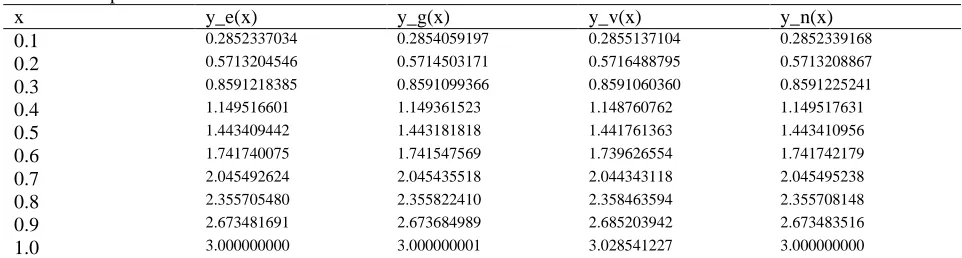
Table 2. Experiment 2
x y_e(x) y_g(x) y_v(x) y_n(x)
0.1 0.2852337034 0.2854059197 0.2855137104 0.2852339168
0.2 0.5713204546 0.5714503171 0.5716488795 0.5713208867
0.3 0.8591218385 0.8591099366 0.8591060360 0.8591225241
0.4 1.149516601 1.149361523 1.148760762 1.149517631
0.5 1.443409442 1.443181818 1.441761363 1.443410956
0.6 1.741740075 1.741547569 1.739626554 1.741742179
0.7 2.045492624 2.045435518 2.044343118 2.045495238
0.8 2.355705480 2.355822410 2.358463594 2.355708148
0.9 2.673481691 2.673684989 2.685203942 2.673483516
1.0 3.000000000 3.000000001 3.028541227 3.000000000
Table 2 shows the exact solution, the Galerkin method, variational iteration method and the variational-fixed point iteration method. It is to be noted that only 3rd
35
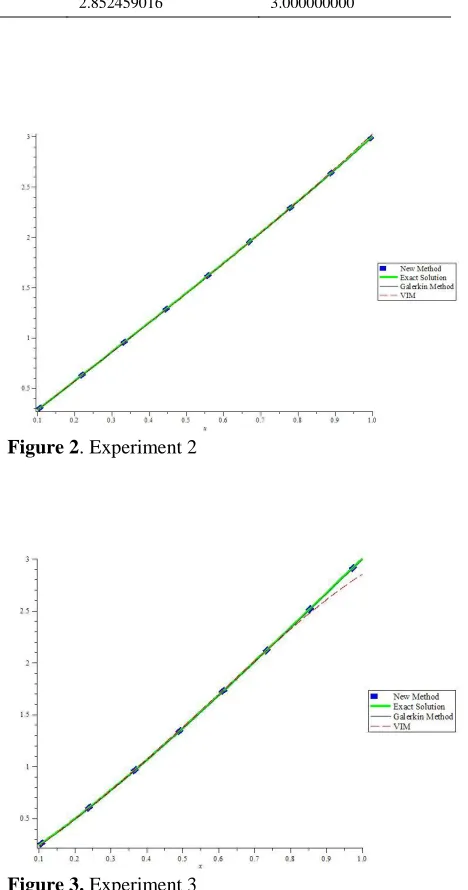
Table 3. Experiment 3x y_e(x) y_g(x) y_v(x) y_n(x)
0.1 0.2363789260 0.2350819672 0.2342704918 0.2363789261
0.2 0.4934462560 0.4924590164 0.4912786885 0.4934462549
0.3 0.7691709690 0.7691803279 0.7698442623 0.7691709685
0.4 1.061308446 1.062295082 1.067016393 1.061308444
0.5 1.367377993 1.368852458 1.378073769 1.367377991
0.6 1.684638024 1.685901640 1.696524591 1.684638022
0.7 2.010058614 2.010491803 2.014106557 2.010058612
0.8 2.340291179 2.339672131 2.320786885 2.340291178
0.9 2.671634964 2.670491803 2.604762295 2.671634964
1.0 3.000000000 3.000000000 2.852459016 3.000000000
Table 3 shows the exact solution, the Galerkin method, variational iteration method and the variational-fixed point iteration technique. It is also noted that only 11th iteration result was used in evaluating the approximate solution, which indicates a super convergence when compared with the exact solution.
CONCLUSION
From the experiments above, as the iteration increases, the error decreases and the rate of convergence of the proposed method increases, and it is also observed that the variational-fixed point iterative technique converges sharply to the exact solution which leads to super convergence. We conclude that the variational-fixed point iterative technique is a very strong and efficient technique for finding the approximate solution of second order linear boundary value problems because it has been proved to have an upper hand over the existing method. Thus we can conclude that the convergence of present method is faster than those in the literature.
Figure 1. Experiment 1
Figure 2. Experiment 2
36
ACKNOWLEDGEMENTThe authors thank the referees for their comments and remarks that helped to improve the presentation of the manuscript. The authors also gratefully acknowledge that this research was partially supported by the Universiti Putra Malaysia (UPM) under the GP-IBT Grant Scheme having project number GP-IBT/2013/9420100.
REFERENCES
Araghi F. M. A., Dogaheh G. S., Sayadi Z., (2011). The Modified Variational Iterational Method for Solving Linear and Nonlinear Ordinary Differential Equations. Australian Journal of Basic and Applied Sciences, 234, 5(10)406-416. ISSN 1991-8178
Daniel T., Rao V.J., Tesfy G., (2012). Boundary Value Problems and Approximates Solutions, MEJS, 4(1),102-114.
He J. H. (2006). Some Asymptotic Methods for Strongly Nonlinear equations. International Journal of Modern Physics, 20(10), 1141-1199.
He J. H., (2007). Variational Iteration method-Some Recent Results and New Interpretations, Journal of Computational and Applied Mathematics, 29(1), 13-17.
He J. H., (2012). Notes on the Optimal Variational Iteration Method, Applied Mathematics Letters, (25) 1579-1581.
He J. H.,(1999). Variational Iteration-A Kind of Nonlinear Analytical Techniques: Some Examples,
International Journal of Nonlinear Mechanics, 34(4),699-708.
He J. H.,(2000). Variational Iteration Method for Autonomous Ordinary Differential System. Applied Mathematics and Computation, 114(2-3), 115-123.
He J.H. (2008). An Elementary Introduction to Recently Developed Asymptotic Methods and Nano mechanics in Textile Engineering. International Journal of Nonlinear Sciences and Numerical Simulation, 22(21), 3487-3578.
Kilicman A.,Wadai M. (2016). On the Solutions of three point boundary value problems using
variational-fixed point iteration method, Math. Sci. (Springer)10(1-2), 33--40.
Lu J., (2007) Variational Iteration Method for Solving Two Point Boundary Value Problems, Journal of Computational and Applied Mathematics, 207(1), 92-95.
Noor M. A., Mohyuddin S.T.,(2008). Variational Iteration For Solving Higher Order Nonlinear Boundary Value Problems Using He’s Polynomials. International Journals of Nonlinear Sciences and Numerical Simulation, 19(2),141-157.