TUTORIALS ON AFRICAN BUFFALO OPTIMIZATION FOR SOLVING THE TRAVELLING SALESMAN PROBLEM

120

TUTORIALS ON AFRICAN BUFFALO OPTIMIZATION FOR SOLVING THE TRAVELLING SALESMAN PROBLEM

Odili J.B, Kahar M.N.M, Anwar S, Ali M Faculty of Computer Systems & Software Engineering,

Universiti Malaysia Pahang, Kuantan 26300, Malaysia

ABSTRACT

The African Buffalo Optimization is a newly designed metaheuristic optimization algorithm inspired by the migration of African buffalos from place to place across the vast African forests, deserts and savannah in search of food. Being a new algorithm, several researchers from different parts of the research world have indicated huge interest in understanding the working of the novel algorithm. This paper presents a practical demonstration of the workings of the African Buffalo Optimization in solving the popular travelling salesman problem. It is our belief that this tutorial paper will be helpful in further introducing the new algorithm and making it user-friendly.

Keywords: Tutorials, African Buffalo Optimization, African buffalos, Travelling Salesman Problem

INTRODUCTION

Optimization, generally, is concerned with the reduction of wasteful input, increased speed and the maximization of profitable output. It can be defined as the economics of science, engineering, technology and industrial concerns since it emphasizes the minimization of input values or resources and the maximization of quality output (Odili, Kahar, & Anwar, 2015). Because of the relevance of optimization in human development, several optimization algorithms have been developed to speed-up industrial, engineering and scientific procedures. Some of the very popular optimization algorithms are the Ant Colony Optimization (Liao, Stützle, de Oca, & Dorigo, 2014), Particle Swarm Optimization (Kennedy, 2011), Artificial Bee Colony Optimization (Akay & Karaboga, 2012) etc. In spite of the very laudable contributions of the existing algorithms, however, it has been observed that there are still need for improvement. Some of the areas that need further improvements include the need for more efficiency in the use of computer resources, effectiveness in obtaining results, simplicity to enhance user-friendliness (Khompatraporn, Pintér, & Zabinsky, 2005) etc. The African Buffalo Optimization (ABO) was developed to complement the existing algorithms in providing the needed improvements.

121

Siegismund, 2012). African buffalos are able to track the rainy season when they obtain the most nutrition in different regions of Africa: east, west, south and north (Smitz et al., 2013). One of the most intriguing qualities of the African buffalos is their ability to harness the collective intelligence of the herd through ‘voting’. Studies have indicated that these animals make important routing decisions through communal decision- making (Conradt & Roper, 2003; Okello et al., 2015).

Utilizing the /waaa/ calls requesting the buffalos to move on to explore safer and/or more rewarding locations and the /maaa/ vocalizations that summons the buffalos to graze at a safe and lush location, the buffalos are able to migrate out of a starving location to a rewarding one (Odili, Kahar, Anwar, & Azrag, 2015). Since its development, the ABO has been quite successful solving the symmetric and asymmetric travelling salesman problem (Odili, Kahar, & Noraziah, 2016), numerical function optimization and tuning the PID Controller parameters of Automatic Voltage Regulators (Odili & Mohmad Kahar, 2016a), hence the need for a tutorial on the workings of the algorithm to make it more user-friendly.

Travelling Salesman Problem

The travelling salesman problem (TSP) is basically the problem of a particular salesman/woman who has customers in different locations and needs to visit each of them to possibly supply them some goods or services and return to his initial location. The main constraint in his trip is that he must visit each location only once and return to the starting location using the cheapest route. The travelling salesman problem could either be asymmetric in which case there exist a difference in costs between the forward or backward route or symmetric where the cost is same on both ways (Gülcü, Mahi, Baykan, & Kodaz, 2016; Odili, 2013)

The rest of this paper is structured as follows: section two presents the African Buffalo Optimization Algorithm; section three discusses the working of the algorithm; section four highlights the practical demonstration of the basic flow of the algorithm to solving the travelling salesman’s problem and section five draws conclusion on the study.

AFRICAN BUFFALO OPTIMIZATION

The ABO algorithm is highlighted in Figure 1. In Figure 1, the wkrepresents the waaa

calls (move on / explore) with particular reference to buffalo k. This call is a signal to the buffalos to move on to a safer or more rewarding location; mkdenotes the maaa call

(stay to exploit) that requests the buffalos; wk′ denotes a request for further exploration

(Odili & Mohmad Kahar, 2016b). Similarly, mk′ represents a requests for further

exploitation; lp1 and lp2 are the learning parameters and 𝜆 is a random number that takes a value of between 0 and 1.

The Working of the ABO

122

best locations (𝑏𝑝. k ) vis-à-vis the target solution. This is done using the first and second equations respectively.

𝑚_𝑘′ = 𝑚_𝑘 + 𝑙𝑝1(𝑏𝑔 – 𝑤_𝑘) + 𝑙𝑝2(𝑏𝑝. 𝑘 − 𝑤_𝑘 ) (1)

𝑤_𝑘′ =(𝑤𝑘+ 𝑚𝑘)

𝜆 (2)

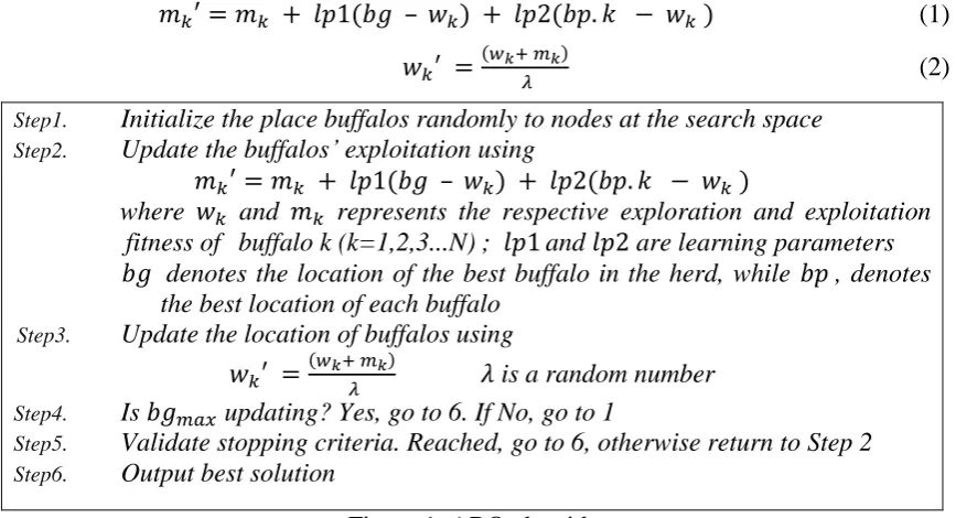
Step1. Initialize the place buffalos randomly to nodes at the search space Step2. Update the buffalos’ exploitation using

𝑚𝑘′ = 𝑚𝑘 + 𝑙𝑝1(𝑏𝑔 – 𝑤𝑘) + 𝑙𝑝2(𝑏𝑝. 𝑘 − 𝑤𝑘 )

where 𝑤_𝑘 and 𝑚_𝑘 represents the respective exploration and exploitation fitness of buffalo k (k=1,2,3...N) ; 𝑙𝑝1 and 𝑙𝑝2 are learning parameters 𝑏𝑔 denotes the location of the best buffalo in the herd, while 𝑏𝑝 , denotes

the best location of each buffalo Step3. Update the location of buffalos using

𝑤_𝑘′ =(𝑤𝑘+ 𝑚𝑘)

𝜆 𝜆 is a random number

Step4. Is 𝑏𝑔_𝑚𝑎𝑥 updating? Yes, go to 6. If No, go to 1

Step5. Validate stopping criteria. Reached, go to 6, otherwise return to Step 2 Step6. Output best solution

Figure 1. ABO algorithm

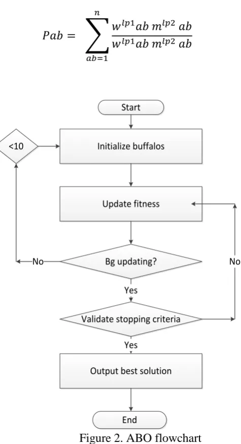
Please note that in each iteration, the algorithm keeps a record of each buffalo’s coordinates. If the buffalos present exploration fitness is superior to the previous individual’s best fitness (𝑏𝑝. k), the algorithm saves the location coordinates for that particular buffalo as its new personal best. Similarly, if the present fitness is superior to the herd’s overall best, the algorithm saves it as the herd’s best (𝑏𝑔). (Odili et al., 2016). After this, it confirms the improvement or otherwise of the leading buffalo (𝑏𝑔). If there is no improvement in the status of the best buffalo (𝑏𝑔) in a number of iteration, then the algorithm re-initializes the entire herd. If the best buffalo is improving its positions, then the algorithm checks to see if the stopping criteria is reached. If the best buffalo fitness (𝑏𝑔) meets our exit criteria, the algorithm terminates and provides the location vector as the solution to the given problem. The stopping criteria could be a specified number of iterations, a specified number of iterations without improvement of the best buffalo etc. The Algorithm flowchart is presented in Figure 2.

ABO for Solving the Travelling Salesman Problem

The ABO solves complex optimization problems using very simple solution steps. The solution steps used for solving the Travelling Salesman Problems are:

(a.) Determine, per some criterion, an initial city for each of the buffalos and place them randomly in those cities.

(b.) Update the fitness of the buffalos using the democratic equation 1 and the decision equation 2, respectively).

(c.) Identify the 𝑏𝑝. k and 𝑏𝑔

123

𝑃𝑎𝑏 = ∑𝑤

𝑙𝑝1_{𝑎𝑏 𝑚}𝑙𝑝2 _𝑎𝑏

𝑤𝑙𝑝1_{𝑎𝑏 𝑚}𝑙𝑝2 _𝑎𝑏 𝑛

𝑎𝑏=1

(3)

Initialize buffalos

Update fitness

Output best solution <10

Validate stopping criteria Bg updating?

Start

End Yes

Yes

No No

Figure 2. ABO flowchart

(e.) Confirm if the 𝑏𝑔 is updating? If yes, go to (f.). If not updating in 10 iterations, go

to (a.)

(f.) Validate stopping criteria? Reached, go to (g.). No, return to (b.) (g.) Output the best solution.

124 Practical Demonstration of ABO for TSP

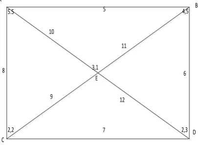
To further illustrate the working of the ABO, let us demonstrate ABO strategy for solving a five-node TSP using seven buffalos. The costs of the edges are indicated against each edge (see Figure 3).

9

5.5 5

10

3,1 11

7 12

2,3 6 8

2,2

4,5 A

B

D C

E

Figure 3. A five-node TSP instance

Assuming the buffalos began the search at node D, it means that they will also terminate the search at the same node. The second assumption is that they took different routes. Let us use the ABO to simulate the movements of the buffalos in solving this problem (See Figures 4-7). The parameters for this tutorials are: lp1=0.6, lp2=0.5,

𝜆=0.5-0.9. For the first iteration, the algorithm picks location E values as the 𝑏𝑔. This decision is randomly made. Please note that in iteration 1, the 𝑏𝑝. k (best location found by each buffalo) is the starting locations of the buffalos

m_k′ = m_k + lp1(𝑏𝑔 – w_k)

+ lp2(𝑏𝑝. k − w_k)

m_k′(𝑥) = 2+0.6(3-2) + 0.5(2-2)

= 2 + 0.6 +0

= 2.6

mk′(𝑦) = 3 + 0.6 (1-2) + 0.5 (3.3)

= 3-0.6

= 2.4

m_k′ = (2.6, 2.4). So new m_k = (2.6, 2.4)

Applying exploration Equation 2

w_k′ =(wk+ mk) 𝜆

w_k′(𝑥) = (2 + 2.6) 0.9

Applying TSP movement Equation 3

𝑃𝑎𝑏 = ∑𝑤

𝑙𝑝1_{𝑎𝑏 𝑚}𝑙𝑝2 _𝑎𝑏

𝑤𝑙𝑝1_{𝑎𝑏 𝑚}𝑙𝑝2 _𝑎𝑏 𝑛

𝑎𝑏=1

= 5.1

0.6 _{𝑥 1 𝑥 2.6}0.5 _{𝑥 1}

60.6 _{𝑥 1 𝑥 2.4}0.5 _{𝑥 1}

The value of ab=1 in the first iteration 2 in the second, 3 in the third etc.

=2.658 2.811

= 0.94

Now multiply by the heuristic values on the graph

125 = 5.1

w_l′(𝑦) = (3+2.4)

0.9

= 6

w_k′ = = (5.1, 6)

= 11.33

The closest value on the TSP graph to 11.33 is 12, so buffalo 𝑘 follows route DE.

Figure 4. Buffalo k’s movement

Plotting the experimental values obtained using Equation 3 to represent buffalo 𝑗, since they are all at the same starting location, we have:

𝑃𝑎𝑏 = ∑𝑤

𝑙𝑝1_{𝑎𝑏 𝑚}𝑙𝑝2 _𝑎𝑏

𝑤𝑙𝑝1_{𝑎𝑏 𝑚}𝑙𝑝2 _𝑎𝑏 𝑛

𝑎𝑏=1

5.10.6𝑥 1 𝑥 2.60.5 𝑥 1

60.6 𝑥 1 𝑥 2.40.5 𝑥 1

= 0.94

Now multiply by the heuristic values on the graph

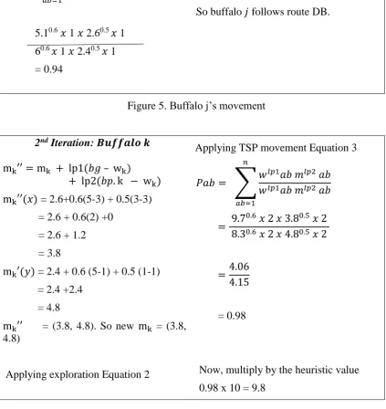
= 0.94 x 6 = 5.64

So buffalo 𝑗 follows route DB.

Figure 5. Buffalo j’s movement

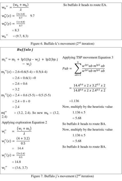
2nd _{Iteration: 𝑩𝒖𝒇𝒇𝒂𝒍𝒐 𝒌}

m_k′′ = m_k + lp1(𝑏𝑔 – w_k) + lp2(𝑏𝑝. k − w_k)

m_k′′(𝑥) = 2.6+0.6(5-3) + 0.5(3-3)

= 2.6 + 0.6(2) +0

= 2.6 + 1.2

= 3.8

m_k′(𝑦) = 2.4 + 0.6 (5-1) + 0.5 (1-1)

= 2.4 +2.4

= 4.8

mk′′ = (3.8, 4.8). So new mk = (3.8,

4.8)

Applying exploration Equation 2

Applying TSP movement Equation 3

𝑃𝑎𝑏 = ∑𝑤

𝑙𝑝1_{𝑎𝑏 𝑚}𝑙𝑝2 _𝑎𝑏

𝑤𝑙𝑝1_{𝑎𝑏 𝑚}𝑙𝑝2 _𝑎𝑏 𝑛

𝑎𝑏=1

= 9.7

0.6 _{𝑥 2 𝑥 3.8}0.5 _{𝑥 2}

8.30.6 _{𝑥 2 𝑥 4.8}0.5 _{𝑥 2}

=4.06 4.15

= 0.98

Now, multiply by the heuristic value

126

w_k′′ =(wk+ mk) 𝜆

w_k′′(𝑥) = (3+3.8)

0.7 = 9.7

w_k′′(𝑦) = (1+4.8)

0.7

= 8.3

w_k′′ = (9.7, 8.3)

So buffalo 𝑘 heads to route EA.

Figure 6. Buffalo k’s movement (2nd iteration)

𝑩𝒖𝒇𝒇𝒂𝒍𝒐 𝒋

mj′′ = mj + lp1(𝑏𝑔 – wj) + lp2(𝑏𝑝. j

− w_j)

mj′′(𝑥) = 2.6+0.6(5-4) + 0.5(4-4)

= 2.6 + 0.6(1) +0

= 2.6 + 0.6

= 3.2

mj′′(𝑦) = 2.4 + 0.6 (5-5) + 0.5 (5-5)

= 2.4 + 0 + 0

= 2.4

mj′′ = (3.2, 2.4). So new m_k = (3.2, 2.4)

Applying exploration Equation 2

w_j′′ = (wj+ mj) 𝜆

w_j′′(𝑥) = (4 + 3.2) 0.5

= 14.4

w_j′′(𝑦) = (5+2.4)

0.5

= 14.8

wj′′ = (3.6, 3.7)

Applying TSP movement Equation 3

𝑃𝑎𝑏 = ∑𝑤

𝑙𝑝1_{𝑎𝑏 𝑚}𝑙𝑝2 _𝑎𝑏

𝑤𝑙𝑝1_{𝑎𝑏 𝑚}𝑙𝑝2 _𝑎𝑏 𝑛

𝑎𝑏=1

= 14.4

0.6 _{𝑥 2 𝑥 3.2}0.5 _{𝑥 2}

14.80.6 _{𝑥 2 𝑥 2.4}0.5 _{𝑥 2}

=1.136

Now, multiply by the heuristic value

1.136 x 5

= 5.68

So buffalo 𝑘 heads to route BA.

Now, multiply by the heuristic value

1.136 x 5

= 5.68

So buffalo 𝑘 heads to route BA.

Figure 7. Buffalo j’s movement (2nd _iteration)

127

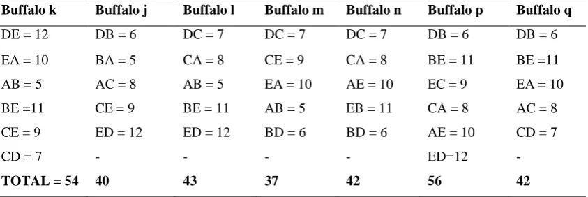
Table 1. Demonstration of symmetric TSP

Buffalo k Buffalo j Buffalo l Buffalo m Buffalo n Buffalo p Buffalo q

DE = 12 DB = 6 DC = 7 DC = 7 DC = 7 DB = 6 DB = 6

EA = 10 BA = 5 CA = 8 CE = 9 CA = 8 BE = 11 BE =11

AB = 5 AC = 8 AB = 5 EA = 10 AE = 10 EC = 9 EA = 10

BE =11 CE = 9 BE = 11 AB = 5 EB = 11 CA = 8 AC = 8

CE = 9 ED = 12 ED = 12 BD = 6 BD = 6 AE = 10 CD = 7

CD = 7 - - - - ED=12 -

TOTAL = 54 40 43 37 42 56 42

From this investigation, it is obvious that the cheapest route is that taken by Buffalo m that has a total cost of 37. So the algorithm outputs that particular route as the best solution.

CONCLUSION

This paper is a tutorial for the newly-designed African Buffalo Optimization algorithm. The paper aims to practically explain the working of the algorithm such that none professionals can appreciate its working and possibly implement it to solve optimization problems. Simplifying algorithms to a level that none experts can use is a necessary requirement in modern optimization design. At the end of this tutorial paper, we believe that our aim has been achieved. Nevertheless, we recommend that the working of the ABO tutorials on other optimization problems such as job-shop scheduling, vehicle routing and global optimization benchmark functions.

ACKNOWLEDGEMENT

The authors are grateful to the Faculty of Computer Systems & Software Engineering for funding this study under Grant GRS 1403118

REFERENCES

Akay, B., & Karaboga, D. (2012). A modified artificial bee colony algorithm for real-parameter optimization. Information Sciences, 192, 120-142.

Conradt, L., & Roper, T. J. (2003). Group decision-making in animals. Nature, 421(6919), 155-158.

Gülcü, Ş., Mahi, M., Baykan, Ö. K., & Kodaz, H. (2016). A parallel cooperative hybrid method based on ant colony optimization and 3-Opt algorithm for solving traveling salesman problem. Soft Computing, 1-17.

128

Khompatraporn, C., Pintér, J. D., & Zabinsky, Z. B. (2005). Comparative assessment of algorithms and software for global optimization. Journal of global optimization, 31(4), 613-633.

Liao, T., Stützle, T., de Oca, M. A. M., & Dorigo, M. (2014). A unified ant colony optimization algorithm for continuous optimization. European Journal of Operational Research, 234(3), 597-609.

Lorenzen, E., Heller, R., & Siegismund, H. R. (2012). Comparative phylogeography of African savannah ungulates. Molecular Ecology, 21(15), 3656-3670.

Odili, J. B. (2013). Application of Ant Colony Optimization to Solving the Traveling Salesman's Problem. Science Journal of Electrical & Electronic Engineering, 2013.

Odili, J. B., Kahar, M. N., & Noraziah, A. (2016). Solving Traveling Salesman’s Problem Using African Buffalo Optimization, Honey Bee Mating Optimization & Lin-Kerninghan Algorithms. World Applied Sciences Journal, 34(7), 911-916.

Odili, J. B., & Kahar, M. N. M. (2015). Numerical Function Optimization Solutions Using the African Buffalo Optimization Algorithm (ABO). British Journal of Mathematics & Computer Science, 10(1), 1-12.

Odili, J. B., Kahar, M. N. M., & Anwar, S. (2015). African Buffalo Optimization: A Swarm-Intelligence Technique. Procedia Computer Science, 76, 443-448.

Odili, J. B., Kahar, M. N. M., Anwar, S., & Azrag, M. A. K. (2015). A comparative study of African Buffalo Optimization and Randomized Insertion Algorithm for asymmetric Travelling Salesman's Problem. Paper presented at the Software Engineering and Computer Systems (ICSECS), 2015 4th International Conference on.

Odili, J. B., & Mohmad Kahar, M. N. (2016a). African Buffalo Optimization Approach to the Design of PID Controller in Automatic Voltage Regulator System.

National Conference for Postgraduate Research, Universiti Malaysia Pahang, September, 2016, 641-648.

Odili, J. B., & Mohmad Kahar, M. N. (2016b). Solving the Traveling Salesman's Problem Using the African Buffalo Optimization. Computational Intelligence and Neuroscience, 2016, 1-12.

Okello, M. M., Kenana, L., Maliti, H., Kiringe, J. W., Kanga, E., Warinwa, F., Kija, H. (2015). Population Status and Trend of Water Dependent Grazers (Buffalo and Waterbuck) in the Kenya-Tanzania Borderland. Natural Resources, 6(02), 91.

Paul, J. D., Roberts, G. G., & White, N. (2014). The African landscape through space and time. Tectonics, 33(6), 898-935.