Consumption, income dynamics and precautionary savings

C onsum ption , Incom e D yn a m ics and

P recau tion ary Savings

L u ig i P is ta fe r r i

Thesis submitted for the degree of Ph.D. in Economics

University College, London

ProQ uest Number: U 6 4 3 4 8 6

All rights reserved

INFORMATION TO ALL U SE R S

The quality of this reproduction is d ep en d en t upon the quality of the copy subm itted. In the unlikely even t that the author did not sen d a com plete manuscript

and there are m issing p a g e s, th e se will be noted. Also, if material had to be rem oved, a note will indicate the deletion.

uest.

ProQ uest U 6 4 3 4 8 6

Published by ProQ uest LLC(2016). Copyright of the Dissertation is held by the Author. All rights reserved.

This work is protected against unauthorized copying under Title 17, United S ta tes C ode. Microform Edition © ProQ uest LLC.

ProQ uest LLC

789 East E isenhow er Parkway P.O. Box 1346

A B S T R A C T

I study the dynamics of household consumption and income. My thesis con­ sists of four papers, detailed as follows.

In the first paper, I test for precautionary savings and excess sensitivity of consumption using a panel of Italian households that has measures of income expectations. The latter provide a powerful instrument for predicting income growth. The empirical analysis allows for a fairly general specification for the stochastic structure of the forecast error. I find that consumption growth is pos­ itively correlated with the expected variance of income and uncorrelated with predicted income growth.

In the second paper, I test for the saving for a rainy day hypothesis using the same set of subjective income expectations described above. According to the permanent income hypothesis, household savings should only react to tran­ sitory income shocks, as permanent shocks are entirely consumed. I show how subjective expectations can help to identify separately the transitory and the permanent shocks to income, thus providing a powerful test of the theory.

In the third paper, I notice th at the theory of full consumption insurance implies absence of consumption mobihty between any time periods. This imph- cation requires knowledge of the evolution of the entire consumption distribution. I test this unexplored prediction of the theory using a panel of Itahan households. I design a non-parametric test and find substantial mobihty of consumption even controlling for possible preference shifts and measurement error. The findings strongly reject the theory of full consumption insurance.

C o n te n ts

1 In tro d u ctio n and background issues 11

M otivation... 11

Consumption and income dynamics... 13

Income dynamics and precautionary sav in g s... 15

Consumption insurance... 18

Data sources ... 19

The Bank of Italy Survey of Household Income and W ealth... 20

The Michigan Panel Study of Income D ynam ics... 21

2 S u b jec tiv e e x p ecta tio n s and th e ex cess se n sitiv ity p u zzle 24 Introduction... 24

Review of the hterature and motivation... 26

Predicting income g ro w th ... 27

The conditional variance of consumption g ro w th ... 29

Non-separability between consumption and leisure... 30

The stochastic structure of the forecast e rro rs...31

Predicting income growth and consumption risk with subjective expectations... 32

Expected income g ro w th ...32

Income risk ... 36

Sample and specification issue... 37

Euler equation estim ates... 40

C onclusions... 45

The estimation strateg y... 53

Income shocks decomposition...53

The effect of transitory and permanent income shocks on s a v in g s 54 Identification... 55

Consistency ...57

Testing for quadratic preferences ...57

Chamberlain’s critique...58

The data and the actual implementation of the t e s t ...59

The empirical distribution of the income shocks... 61

Empirical results ... 63

Testing for Chamberlain’s critique...6 8 C onclusions... 69

4 C on su m p tion insurance or co n su m p tio n m ob ility? 76 Introduction... 76

Consumption in su ran ce... 79

Consumption m o b ility ... 80

E x ten sion s... 82

Preference specification and heterogeneity... 82

Measurement erro r... 85

The d a t a ...8 6 Empirical results ... 87

Pull sample e stim ate s... 87

Preference specification and heterogeneity... 89

Measurement e rro r... 91

Sub-sample e stim a te s... 95

C onclusions ... 96

Modelling the distribution of earn in g s... 107

A brief survey of the lite ra tu re ... 107

Aspects of the distribution of earnings... 109

The conditional mean of earnings... 110

The conditional variance of earnings... 114

The validity of the instrum ents... 119

Asymmetry and the lack of identification ... 1 2 0 The d a t a ... 121

Empirical r e s u lts ... 123

Model A ... 123

Model B ... 126

The conditional m e a n ... 126

The structure of the error te r m ... 129

The identification of the ARCH coefficients ... 131

The conditional variance of the transitory shock... 133

The conditional variance of the permanent sh o ck ... 134

The implications of the empirical e stim ate s... 136

A general discussion... 136

Precautionary savings and insurance... 139

C onclusions... 143

6 C on clu sion s 155

No part of this thesis has been presented before to any University or Col­ lege for submission as part of a higher degree.

A C K N O W L E D G M E N T S

I am greatly indebted to Costas Meghir, my Principal Supervisor, and Orazio Attanasio, my Subsidiary Supervisor at University College London, for assiduous suggestions, intuitions and encouragement. Tullio Jappelli deserves a special mention for his generosity and constant support.

Part of this thesis draws from joint work with Tullio Jappelli and Costas Meghir. I would like to thank James Banks, Richard Blundell, François Bour- gouignon, Christopher Carroll, Victoria Chick, Angus Deaton, Mika I. Kuisma- nen, Hamish Low, Sidney Ludvigson, Mario Padula, Jonathan Parker, Christina Paxson, Andrea Tiseno, Gughelmo Weber, two anonymous referees and seminar participants at various universities in Europe and the US for useful suggestions and comments.

For intellectual stimulus and moral support received at various stages of my doctorate, I would like to thank my parents and sibhngs, Kazu Araki, Luca Bene- dini. Eve Caroh, Giacinta Cestone, Teresa Delgado, Enzo Formisano, Charles Grant, Luigi Guiso, Marco Pagano, Monica Paiella and Alfonso Rosolia.

Financial support received from Istituto Universitario Navale of Naples, the Italian Ministry of Universities and Scientific Research, the James Lanner Memo­ rial Fund, and the Ente per gli studi monetari bancari e finanziari “Luigi Ein- audi” is gratefully acknowledged.

1

Introduction and background issues

1

M o tiv a tio n

In this dissertation I analyse consumption and savings decisions in the pres­ ence of individual income dynamics. In this introductory chapter I will motivate my line of research and discuss the theoretical models th at lie in the background of the empirical analyses to be presented in Chapters 2 through 5. The discussion is not meant to be exhaustive; the modern theory of intertemporal consumption choice has been recently surveyed, among others, by Deaton (1992b), Browning and Lusardi (1996) and Attanasio (1999); I refer the interested reader to these excellent pieces of work for a more detailed theoretical treatment.

face data-related problems, the most relevant one probably being the so-called Chamberlain’s critique (1984). This is essentially a problem deriving from the inconsistency of empirical estimates in short panels.

I approach these problems with some ingenuity. First, I note that Chamber­ lain’s critique can be attenuated, if not entirely controlled for, by exploiting data on individual subjective expectations. Second, heterogeneity in preferences and individual resources can be accounted for in a fairly general way. In particular, I consider the possibility of accounting for heterogeneneity in income uncertainty. As I win argue in chapter 5, this may have far reaching imphcations not only on partial equilibrium individual consumption choices but also on the general equilibrium of the economy.

I consider testing for three different theoretical propositions. While tests for such propositions are not novel in the empirical literature, my approach is orig­ inal because (i) I exploit data th a t are rarely available to the econometrician, and (ii) the actual format of my tests is different from that proposed so far in the hterature. According to the first proposition, consumption growth does not react to predicted income growth; a test of this proposition, also known as excess sensitivity test, is presented in chapter 2. According to the second proposition, consumption reacts very strongly to unanticipated permanent income changes, b ut very weakly to unanticipated transitory income changes; this is the test I per­ form in chapter 3. Finally, the third proposition states th at consumption does not react to idiosyncratic shocks but only to aggregate unanticipated fluctuations; this is the essence of the full consumption insurance hypothesis. A test for such proposition is presented in chapter 4. The modem theory of consumption choices under incomplete markets provide a rationale for the precautionary motive for saving, i.e. individuals wiU save in the face of uncertain income prospects. In this context, it is important to model and measure income uncertainty. I analyse statistical models for income risk in chapter 5.

I will start by making explicit the relationship between consumption choices and income dynamics. Consider the standard problem solved by an infinitely lived agent i:

subject to the budget constraint:

û^tt+T+i — (l 4- r) + yit-\-T ~ Qt+r) (2)

and the transversahty condition ( “no-Ponzi-game” condition) :

Initial wealth is given. The agent is assumed to hold preferences over non durable consumption, Cit+r. The first order conditions for this problem lead to the Euler equation:

(^t+ i) ( 4

To specialize the solution, I assume that preferences are quadratic, so that u(c) = — ^ a c — and r = 5 for simplicity. This yields the traditional prediction that consumption is a martingale, i.e. th at the change in consumption is an innovation, and therefore orthogonal to all past information:

(^)

as in Hall (1978). A more complicated version of this orthogonality condition is considered and tested in chapter 2. The Euler equation and the intertemporal budget constraint imply the following consumption function:

Cit = a it+ 2 ^, Et {yit+r)

tainty of the model. If income is the only source of uncertainty of the model, one can derive the exact form of the consumption innovation '0. In particular:

< ’ >

To obtain a relationship between consumption innovation and income inno­ vations one needs to specify a stochastic process for income. If income is weU described by an ARMA{1^ 1) process of the form:

V i t + T — 'î^it+T (8 )

'^it+T — P'^it+T—1 d" (9)

with p < 1, it follows th a t income is a stochastic process stationary in levels and

the consumption innovation can be written as:

= ( l + r ) | r + r - p ) ^ “ (1 0)

Of course the two special cases of Ai?(l) and M A{1) are obtained by setting ^ = 0 and p = 0, respectively. W hether a shock is transitory or permanent depends upon the value of p. In particular, if p = 0 all shocks to income are transitory; if, instead, p 1, all shocks become permanent. The marginal

propensity to consume out of the income shock is then implicitly governed by the amount of persistence in the income process, measured by the autoregressive coefficient p. This is somehow inconvenient, as it does not allow a full distinction between shocks th at are mean reverting and shocks th at are not. To this aim, one needs to make explicit the distinction between the two. One option available is to consider income as the sum of two components:

Vit+T — Pit+T 4- Sit+T (if)

Vit+T — Vit+T—\ 4" Cit+r (12)

where C,u+t is serially uncorrelated. Thus:

V i t + T = V i t + T - l + C i t + T 4- £ i t + T — £ i t + T - l (13) Transitory shocks to individual productivity include overtime labour supply, piece-rate compensation, bonuses and premia, etc.; in general, such shocks are mean reverting, e.g. their effect does not last long. On the other hand, some of the innovations to earnings are highly persistent or non-mean reverting, e.g. their effect cumulates over time. Example of permanent innovations are associated to job mobility, long-term unemployment or promotions. The original decompo­ sition of income shocks into transitory and permanent components dates back to Friedman (1957). This practice has become quite standard. Quah (1990) shows th at distinguishing between shocks of different nature may also provide an explanation for the excess smoothness puzzle.

W ith this process, and the additional assumption th at the transitory and the permanent shock are uncorrelated at aU leads and lags, the consumption innovation is:

A cit = i)it = - T ^ £ i t 4- Cit (14)

The optimal rule for the agent is to respond on a one-for-one basis to shocks th at alter the permanent component of income, but to a much lower extent to shocks that affect income only transitorily (namely, to an amount given by the annuity value). This is the income process th at I consider in Chapter 3. A more complicated version of this income process (in logs) is specified and tested in chapter 5.

3

I n c o m e d y n a m ic s a n d p r e c a u tio n a r y sa v in g s

uncorrelated transitory shock (i.e., equations 1 1-1 2). As in Caballero, the only

source of uncertainty of the model is that related to labour income. Suppose th at the problem under study is again given by (1-3), with an given.

Assume however that preferences are of the CARA type: u(c) =

The main advantage of CARA preferences is th at an analytic solution for con­ sumption can be easily derived even under precautionary savings (which obtains if > 0, a case contemplated by CARA or CRRA preferences, but not by quadratic preferences).^ On the other hand, this assumption has at least two problems. The first is that a solution of negative consumption can be optimal for the agent (see Weill, 1992); the second is th at risk aversion is, by assumption, constant. The reaction to risk is therefore unaffected by the level of wealth. While the first problem is much more difficult to tackle,^ one might think of attenuating the second by stratifying the available sample according to some ex­ ogenous characteristics that make the assumption of constant risk aversion less untenable within strata. For instance, the sample could be stratified according to the level of education of the head or initial family income. In both cases, wealth levels will be presumably less dispersed.

Assuming r = S, the Euler equation of this problem is:

= Et

The feed-back solution that satisfies (15) is:

(15)

Cit+1 — Tit + Cit -f '0Ü+ 1 (Ifi)

where Fit = ^ In E t , and 'ipu+i is again the consumption innovation. To find the distribution of the latter, one needs to specify income dynamics.

The ex-post intertemporal budget constraint, (1 + (cit+r — Vü+t) = an, can be alternatively written as follows (Caballero, 1990):

^However, if preferences are CARA the consumption function fails to be concave in the

absence of interest rate risk (Carroll and Kimball, 1996).

^Inserting a non-negativity constraint on consumption amounts to impose a never declining

Cit+T [Vit+T (2 /it+ r )] , Et{yitJ^r) _ / I 4" f /ir A

S ô ^ “S

ÔT7F

= “‘‘+5 irT7F = l“ J''“

Using the income process (11)-(12), one obtains:

% E?=o (1 + r)-" + E S

(1 + r)-^ EJ

Tit+J-I + E

(1 + r)-" EJ=i

—

(1 + ^) ^

(1+r) ^

=

{ ¥ ) v f t

(18) Taking expectations conditional on the information available at time t and rear­ ranging yields the consumption function:

which differs from (6) because of a term that takes into account the effect of

the dispersion of the path of future income on current consumption: more risk will depress current consumption and prompt savings. The relation between the consumption innovation and the labour income innovation can be identified by replacing back cu in (18), obtaining the condition:

1 + ^ Cit+T , 1 ^ it+ T ~ E t (T ^t+T) _ ^

{ i + r v ~ - h ô T T r (^=0)

In the absence of heteroschedasticity (i.e., Et (C^+t-) = cr‘^ and Et {^u+t) ~ for all r), the only relation between consumption innovations and labour income innovations th at satisfies the expression (2 0) is therefore:

'4’it+r — Czi+T T ^ (21)

Given that: Fit = ^]n Et e , one can take a second-order Taylor ex­ pansion of e around the conditional mean of V^it+i to obtain:

^-d^it+i = 1 _ 9xpit+i + + rem . (2 2)

~ 1 + (23)

for infinitesimal risks one obtains:

r u ^ l

,1 4- r

The Euler equation can then be written as:^

(24)

e

-+ ( r -+ 7 ) ^ (25)

This is the Euler equation th at prevails in the presence of a precautionary motive for saving (Kimball, 1990). I estimate a version of equation (25) based on CRRA preferences and accounting for the variance term in chapter 2. In chapter 5 I consider the possibihty th at income shocks are conditionally heteroscedastic.

4

C o n s u m p tio n in su r a n c e

In this section I will describe the main insight of the full consumption insur­ ance hypothesis, for which I will test in chapter 4. As emphasised by Cochrane (1990), full consumption insurance has little to do with self insurance through, say, precautionary savings. These are two different propositions: while the first involves substitution of consumption across states, the second involves substitu­ tion of consumption over time.

Suppose that agents have identical preferences of the CRRA type, u{c) =

( 1 — . Under complete markets, as is known, the social planner’s so­

lution will coincide with that obtained by considering the behavior of the fully decentralized economy. I wiU focus on the former for a m atter of convenience. If the social planner maximizes a weighted sum of individual households’ utihties, the Lagrangian of the problem can be written as (Deaton, 1997):

Z/ =

^

XIX)

i 3 t 3 t \ i J

where i, 5 and t are subscripts for the agent i in the state of nature 5 in period t,

Xi is the social weight for agent z, figt is the Lagrange multiplier associated with the resource constraint, TTgt the probability of state s in time period t, and Cgt aggregate consumption in state s and time t.

The first order condition can be w ritten in logarithms as:

- 7 In Cigt = In /Xst - In Ai - In iTgt (26)

To obtain the rate of growth of consumption, one subtracts side-by-side from the expression at time t -\-l:

A lncit+i = - 7” ^A ln ^t+ i + 7~^Aln7rt+i (27)

where I drop the subscript s because only one state is realized in each period. The two terms on the right-hand-side of equation (27) represent aggregate effects. The first is the growth rate of the Lagrange multipher, the second is the growth rate of the state probabilities. Note th at first-differencing has eliminated all household fixed effects.

Versions of equation (27) have been used to test for the assumption of com­ plete markets. If this assumption holds, only aggregate shocks but not idiosyn­ cratic shocks should m atter for consumption growth, as the latter are fully in­ sured through state-contingent contracts or other informal mechanisms. I present a novel way to test for this imphcation in chapter 5, based on the observation th at full consumption insurance implies absence of consumption mobility.

5

D a t a s o u r c e s

to Hill (1986) for information concerning the Panel Study of Income Dynamics (PSID).

5.1 T h e B an k o f Ita ly S u rvey o f H ou seh old Incom e and W ealth

The SHIW was conducted yearly beginning in 1966. Since 1987 is conducted every other year. The last available survey refers to 1995. In chapter 2 through 5 1 will use SHIW panel data available from 1987 to 1995; 1 will thus omit the description of the characteristics of the survey before 1987. See Brandolini (1998) for more details concerning the historical development of the SHIW.

The basic SHIW sampling unit is the de facto family, i.e. a group of individu­ als linked by blood, marriage or affection, sharing the same dwelling and poohng totally or partially their resources. Institutional population is not included. In­ dividuals who live together exclusively for economic reasons are not considered members of the same family, while in contrast only one unit is recorded in the case of extended famihes. For such reasons, SHlW-based estimates of average family size tend to exceed the corresponding Census estimates.

The design of the SHIW is such th at the samphng procedure occurs in two stages, with municipahties selected in the first stage and families in the second. Municipahties are divided into 51 strata (i.e., 17 regions*3 classes of population size'^). Municipalities in the first class are always included; the selection of those in the other two classes is random, with probability that has been proportional to demographic size in 1987 and constant since 1989. Families are selected from the registry office records. The sample size is roughly 8,000 in aU the survey years 1 consider. Few modifications have affected representativeness; in 1987, for instance, there was an over-samphng of high-income units.

Since 1989 the SHIW includes a rotating panel component. The proportion of panel families has increased over time from 15 per cent (1989) to about 45 per cent (1995); some of the famihes are also re-interviewed in all last four surveys. Panel families are selected with criteria similar to those described above; however, since 1991 participation is on a voluntary basis, i.e. only famihes that express

their willingness to being re-interviewed are contacted.

The survey is carried out by a private company on behalf of the Bank of Italy. D ata are collected in personal interviews, usually between March and May; d ata on income, consumption and wealth refer to the previous calendar year (in Italy this also coincides with the fiscal year). The gross response rate varies substantially over time; it was 60 per cent in 1987, but it dropped to less than 40 per cent in both 1989 and 1991; since then, has been slightly above 50 per cent. Questionnaires are assessed for reliability and consistency by the Bank of Italy statisticians.

Each survey contains special sections whose scope is to study in detail specific subjects (e.g. intergenerational transfers of wealth, use of health, educational and transport services, social mobility, subjective evaluation of working conditions and future income). The expenditure for durable and non durable goods are available in all years. Estimates of households real estate are also available for all surveys and are based on definitions kept largely unchanged over the years. The basic definitions of income and its components is similar to th at used in compiling national accounts; income is recorded net of taxes and social security contributions.

The results of the SHIW are illustrated and commented in the official Bank of Italys publications; the tapes containing microdata are later released in public- use files available free of charge for institutions and researchers in Italy and abroad. As a result, the SHIW is extensively used to study various aspects concerning the behaviour of Itahan households.

5 .2 T h e M ichigan P a n el S tu d y o f Incom e D yn am ics

The Panel Study of Income Dynamics (PSID) is a longitudinal study of a sample of US individuals (men, women, and children) and the family units in which they reside. The study is conducted by the Survey Research Center at the Institute for Social Research (University of Michigan).

core sample), and about 2,000 were low-income families (the Census Bureau’s SEO sample). Since then, individuals from the original households have been reinterviewed every year, irrespective of their living in the same dwelling or with the same people. Adults have been followed as they have grown older, and chil­ dren have been observed as they advance through childhood and into adulthood, forming households of their own (so called split-off households). Information about the original 1968 sample individuals and their co-residents is collected each year (mainly by phone). In order to keep track of demographic changes in the underlying population due to immigration patterns and to increase the rep­ resentativeness of the sample, in 1990 a representative national sample of 2,000 Latino households was added.

The PSID collects information at both family and individual level; moreover, it also includes information about the areas where sample units live (unem­ ployment rates, food needs, etc.). The core of the survey is to collect data of economic and demographic content, with attention paid in particular to income sources and amounts, employment, family composition changes, and residential location; however, in some waves of the study a set of sociological or psycho­ logical questions are also asked. Information gathered in the survey applies to the circumstances of the family unit as a whole (e.g., type of housing) or to par­ ticular persons in the family unit (e.g., age, earnings). While some information is collected about all individuals in the family unit, the greatest level of detail is ascertained for the primary adults heading the family unit. O ther important topics covered by the PSID include housing and food expenditures, housework time, and health status.

from roomers and boarders or business income,^ Education level is computed using the PSID variable with the same name.

® As noted by Grottshalk and Moffitt (1993), the measure of labour income available in the

PSID has sources that may reflect capital income, such as the labour part of farm income and

2

Subjective expectations and the excess

sensitivity puzzle

1

I n tr o d u c tio n

An important implication of the permanent income hypothesis is th at indi­ vidual consumption growth should not respond to expected income growth. The certainty-equivalence version of the model also suggests th at consumers do not react to income risk. But for applied economics the fundamental problem is measuring income risk and predicting future income on the basis of variables th at are in individuals’ information set and can be observed by the econometri­ cian. In this chapter I test the theory of intertemporal consumers choices using d ata on subjective income expectations to predict realized income growth. The advantage is th at no assumption about the process th at generates income is re­ quired. In the Euler equation I also control explicitly for the potential effect of income risk, predictable changes in households labor supply, and the nature of the aggregate shocks.

mea-sures of subjective income and inflation expectations, an annual measure of non­ durable consumption that is not affected by seasonality factors, and a wealth of information on financial and real assets. The availability of a good measure of as­ sets is particularly useful for checking for the possibility of asymmetric response of consumption to predicted income growth.

To date, the panel component of the SHIW has not been extensively exploited for econometric purposes. For the purpose at hand, the main limitation of the panel is that it is relatively short. Even though over long periods of time the forecast error in consumption growth should be zero on average, in my case it may not. In short panels the null hypothesis that the coefficient of predicted income growth in the Euler equation is zero is a joint test of the orthogonality condition implied by the permanent income hypothesis and of the maintained assumptions about the particular stochastic structure of the forecast error. Rejection of the null could be attributed either to a failure of the theory or to the inconsistency of the estimator in short panels. My test must therefore be designed to tackle this important econometric problem.

In Section 2 I review the literature on excess sensitivity tests, motivate the methodology and describe how it differs from alternative approaches. The con­ struction of subjective income expectation is presented in Section 3. Here I also compare income expectations with income realizations and discuss the validity of expectations as an instrument for predicting realizations. Data and specifi­ cation issues are discussed in Section 4. Euler equation estimates, reported in Section 5, indicate th a t consumption growth is positively correlated with the expected variance of income growth, but uncorrelated with predicted income growth. To check for possible asymmetries in the response of consumption to predicted income growth, I also split the sample according to the level of assets (as in Zeldes, 1989a) and distinguish between positive and negative expected income growth (as in Shea, 1995). In short, I cannot reject the orthogonality conditions imphed by intertemporal optimization, but can reject the certainty equivalence version of the permanent income hypothesis. Section 6 summarizes

showing the pervasiveness of borrowing constraints in the Italian economy.

2

R e v ie w o f t h e lite r a tu r e a n d m o tiv a tio n

Several authors have tested the permanent income hypothesis by estimating versions of the following Euler equation with panel data:

Alncit+i =

a!^Fit+i-\-p~^{Eitrit+i-8)-\-uarit(AInCit+i - + /?EitAlnyit+i + ^zt+i

where 2 is a household index, Cjt+i a measure of non-durable consumption, Fit-\-\

includes predictable indicators of households’ preferences (such as age), ra+i is the real after-tax rate of interest, p~^ the intertemporal elasticity of substitu­ tion, 6 the rate of time preferences. En the expectation operator and sn ^i the forecast error. Equation (1) can be derived exactly assuming th a t preferences

are of the isoelastic form and that the distribution of the real interest rate and of consumption growth is jointly lognormal. Alternatively, it can be regarded as a second-order approximation to the first-order conditions of the consumer optimization problem.

Predicted income growth is often added to the Euler equation in order to test the orthogonality condition implied by intertemporal optimization, i.e. that EitA lnj/it+i should not help in explaining consumption growth (/? = 0). It should be noted th at the excess sensitivity test I perform has power against some, but not aU, alternative consumption models. For instance, while myopic behavior will lead to excess sensitivity in every period, in a model with prudence and borrowing constraints the orthogonality condition may not be violated most of the time (and even perhaps aU the time), as households save in the antici­ pation of future constraints. Empirically, it is very hard to distinguish between precautionary saving and models with liquidity constraints.

tional variance of the uncertain components - consumption and the real interest rate - is difficult to observe and is therefore generally omitted from the esti­ mation. Third, excess sensitivity may result from a failure to control properly for non-separability between consumption and leisure. Finally, excess sensitivity may also arise spuriously from the mispecification of the stochastic structure of forecast errors. I address these four problems in turn.

2.1 P r ed ic tin g in com e grow th

Testing for excess sensitivity requires reliable instruments to predict income growth. However, finding such instruments in panel data has proved to be ex­ tremely difficult, particularly in US studies. The Panel Study of Income Dy­ namics (PSID), which has been extensively used to estimate Euler equations, has relatively good data on income but information on consumption is limited to food expenditures. The Consumer Expenditure Survey (CEX) does give de­ tailed measures of consumption, but the information on income is scanty and suffers from severe measurement error. Three approaches have been proposed to enhance the power of the instruments: out-of-sample information, two-sample instrumental variables techniques, and subjective income expectations.

Shea (1995) isolates a subset of households in the PSID whose heads can be matched to labor union contracts. Information on these contracts is then used to construct a measure of expected nominal wage growth. The latter is found to be strongly correlated with actual wage growth (a coefficient of 0 . 8 6 with a (-statistic

of 3.8). Inflation expectations, however, are estimated on aggregate data through an autoregressive forecasting model. Shea then estimates an equation similar to (1) omitting the conditional variance term and replacing the income term with

the expected real wage growth of the household head. He finds th a t expected wage declines affect consumption more strongly than expected wage increases, a result th at is not consistent with either myopia or with the hypothesis th at excess sensitivity is due to liquidity constraints.® There are several problems with this

® Garcia, Lusardi and Ng (1997) apply a switching regression model with unknown sample

approach. One is th at it assumes th at the history of past inflation is known to each households in the sample. Another is that Shea ends up w ith a small sample (647 consumption changes drawn from 285 households), often resulting in poor standard errors, particularly if the sample is split according to the asset-income ratio.^ Finally, since only food consumption is available in the PSID, he requires an assumption of separability between food and other non-durable expenditures in the household utility function. Yet as Attanasio and Weber (1995) point out, this assumption is rejected in the CEX.

A second possibility is to enhance the power of the test by using two-sample instrumental variable techniques. Lusardi (1996) uses consumption data from the CEX and income data from the PSID, thus overcoming the problem of using just food consumption to estimate the Euler equation. The data are matched by a two-sample instrumental variable estimator. Nonetheless, the adjusted Fi? of the regressions of actual income growth on the instruments (demographic variables, education and occupation dummies) is only about 1 percent (see Lusardi, 1996, Table 4). Even though Lusardi finds evidence of excess sensitivity to predicted income growth, she does not investigate whether excess sensitivity arises from non-separabilities, myopia, liquidity constraints or other sources.

Hayashi’s (1985) and Flavin’s (1994) approach is the closest in spirit to the one I use in this study. Hayashi uses a unique data set of Japanese households re­ porting subjective expectations for income and consumption on a quarterly basis. He derives the theoretical covariance between the forecast errors in consumption growth and the subjective income expectations, estimates the parameters of the Euler equation by applying a minimum distance estimator and finds some evi­ dence in favour of excess sensitivity. The procedure does not require assumptions about the nature of the aggregate shocks, and is therefore consistent even in short panels.

The 1967-69 US Survey of Consumer Finances used by Flavin contains a

cate-^The effect of expected real wage growth is never significantly different from zero in the

regressions in Table 5, p. 195. When Shea splits expected income according to positive and

negative expected wage growth he finds an implausible coefficient of 2.242 for expected wage

gorical variable about expectations of family income changes. These, in addition to lagged disposable income, are used as an instrument for income growth. Using a robust instrumental variable estimator to control for the presence of influential outliers. Flavin finds evidence of excess sensitivity for both high and low asset households. Evaluating the overall predictive power of Flavin’s instrument is not easy, because first-stage results are not fully reported. Data are again problem­ atic in this application. The Survey does not contain a consumption measure, which must therefore be inferred from income and assets. The sample size is small (774 observations), especially when the sample is split by assets.

2.2 T h e con d ition al variance o f co n su m p tio n grow th

The conditional variance term in equation (1) is generally omitted from the

estimation.® This is correct only under the certainty equivalence version of the model, which imphes th at households do not react to the expected variance of consumption growth. However, if the utility function exhibits decreasing risk aversion, prudent households react to expected consumption risk by reducing consumption in period t relative to period t 4- 1, to an extent th a t depends on

the degree of prudence.® The reason the variance term is omitted in actual estimation is not th at applied researchers beheve in quadratic utility.^® Rather, it is th at it has turned out to be extremely difficult to find suitable proxies for the conditional variance.

If the conditional variance term is omitted, one cannot of course test for quadratic preferences or estimate the degree of prudence. But the consequences of this omission could be far more serious. Ludvigson and Paxson (1997) point out that estimating a linearised Euler equation can bias the coefficient of the intertemporal rate of substitution. Furthermore, insofar as the conditional

vari-®A notable exception is Dynan (1993).

^Kimball (1990) defines absolute prudence as the ratio between the third derivative and

the second derivative of the within-period utility function. With isoelastic preferences, relative

prudence —U"'/cU'' equals 1 plus relative risk aversion.

^°Research on precautionary saving is in fact steadily growing, see Browning and Lusardi

ance of consumption is correlated with the latter will proxy for the omitted effect of consumption risk, generating spurious evidence of excess sensitivity. Carroll (1992) goes one step further, and points out th a t even Zeldes’ (1989a) sample splitting approach may produce spurious evidence in favour of liquidity constraints if one does not control properly for expected consumption risk. In fact, Zeldes’ test consists in splitting the sample according to the asset- income ratio: if hquidity constraints are at the root of excess sensitivity, one should find no violation of the orthogonality conditions in the high-asset, and excess sensitivity in the low-asset group. But omitting the conditional variance term creates a spurious correlation between consumption growth and income th at is stronger for low-wealth households. The reason is that rich households have greater capacity than poor ones to buffer income fluctuations by drawing down their assets, so th at a finding of excess sensitivity in the group of poor households only - as in Zeldes - could be rationalized once the assumption of certainty equivalence is dropped by the theory of intertemporal choices.

There are two ways to solve the problem. One would be to estimate the non-hnear Euler equation by the generalized method of moments. The second, which is used here, is to introduce explicit proxies for the conditional variance of consumption in the linearised Euler equation. This approach is more directly comparable with previous studies; it also allows me to use standard statistical tools to test if preferences are quadratic or if households react to expected income risk.

2.3 N on -sep a ra b ility b etw een co n su m p tio n and leisu re

point has been forcefully made by Attanasio and Weber (1995) and Meghir and Weber (1996) with CEX data. But the same authors also indicate a way out to this problem. Following their suggestions, I augment equation (1) with labor supply indicators.

2 .4 T h e sto ch a stic stru ctu re o f th e forecast errors

The disturbance term in equation (1) is a forecast error, the difference

between realized and expected consumption growth. According to the permanent income hypothesis with rational expectations, the conditional expectation of a forecast error must be zero, i.e. Eit{£it-\-i) = 0. The empirical analog of this expectation is an average taken over long periods of time, not across a large number of households. In fact, as pointed out by Chamberlain (1984), there is no guarantee th at the cross-sectional average of forecast errors will converge to zero as the dimension of the cross-section gets large. For instance, if the forecast error is the sum of an aggregate and of an idiosyncratic shock, then in a short panel the orthogonality condition fails even if the permanent income model is true: aggregate shocks induce a cross-sectional correlation between expected consumption growth and predicted income growth. The problem is sometimes handled by including time dummies in the Euler equation. This approach is restrictive, because it rules out that aggregate shocks are not evenly distributed in the population.

For this reason, excess sensitivity tests performed on short panels are in fact joint tests of the null hypothesis th at ^ = 0 and the stochastic structure of the

forecast error has a known form (so that the distance between the true forecast error and its empirical analog can be suitably adjusted). Rejection of the nuU need not be interpreted as the failure of the theory, but could also be attributed to mispecification of the stochastic structure of the forecast e rro r.D istin g u ish in g between the two alternatives is difficult, unless the true structure of the forecast error is known. Yet, as will be seen, subjective expectations provide a guide to

Deaton (1992, p. 147-48) provides an example with non-additive aggregate shocks leeiding

modelling the stochastic structure of the forecast error, thereby diminishing the problems one faces when testing for excess sensitivity with short panels,

3

P r e d ic tin g in c o m e g r o w th a n d c o n s u m p tio n risk

w it h s u b j e c tiv e e x p e c ta t io n s

I estimate the Euler equation using the 1989-1993 panel section of the Bank of Italy Survey of Household Income and Wealth (SHIW), Details on sample design, response rates and timing of the interviews have been provided in chapter 1. Here I describe only the wording of the questions and the subjective expectations used to predict income growth and to proxy for consumption risk.^^ Several surveys contain subjective income expectations, but vary considerably as to the way expectations are ehcited.^^ In the case of the SHIW, in 1989 and 1991 each labor income and pension recipient interviewed was asked to attribute probability weights, summing to 1 0 0, to given intervals of inflation and nominal income

increases one year ahead,

3.1 E x p ected in com e grow th

In 1989 and 1991 the following two questions were asked to each labour income recipient.

Inflation expectations: “On this table [a table is shown to the respondent] we have indicated some classes of inflation. We are interested in knowing your opinion about inflation twelve months from now. Suppose th at you have 100 points to be distributed between these intervals. Are there intervals you deflnitely

^^Guiso, JappeUi and Terlizzese (1992) used the same SHIW questions to study the effect of

earnings risk on 1989 saving and households’ wealth. They also discuss the pros and cons of

using subjective income expectations,

^^The 1982 Japanese Survey of Family Consumption contains information about consumption

and income expectations. The Dutch VSB Panel, the 1967 US Survey of Consumer Finances,

and the US Survey of Economic Expectations (SEE) contain information on income prospects,

but not on expected or actual consumption. Das and Van Soest (1997) and Dominitz and

Manski (1998) using the VSB and the SEE, respectively, compjare income expectations with

exclude? Assign zero points to these intervals. How many points do you assign to each of the remaining intervals?” For this and the following question the intervals on the table shown to the person interviewed are: less than zero; 0-3; 3-5; 5-6; 6-7; 7-8; 8-10; 10-13; 13-15; 15-20; 20-25; >25 percent. If the response is “less than zero” , the person is asked: “How much less than zero? How many points would you assign to this class?”

Income expectations: “We are also interested in knowing your opinion about your labour earnings or pensions twelve months from now. Suppose th a t you have 1 0 0 points to be distributed between these intervals [a table is shown again].

Are there intervals you definitely exclude? Assign zero points to these intervals. How many points do you assign to each of the remaining intervals?” To construct subjective expectations and variances of the variable of interest (either the rate of growth of nominal earnings or the rate of inflation), I set the upper bound of the distribution -the open interval- at 35 percent. Let xa be the variable of interest. The subjective expectation of xa at time Z —l i s then given by:

K

E {xit\Q-it-\) = ^ [Pr(xfc-i < Xit < Xk)] 2"^ (xfc -1-Xfc+i) fc = l

and the subjective variance by:

K , 2

Var ^ [Pr {xk-\ < xu < z&)] 2 ^ Xk+i) - E {xit\Vtit-i) fc=l

where x^ and xq are, respectively, the upper and the lower bound of the dis­ tribution. Note th at the intervals are not of the same size.^** Since I do not attem pt to estimate the variance within each interval, the conditional variance V ar{xit\Çtit-\) is equal to zero for those reporting point expectations.

Let EitZit^i denote the expected growth rate of nominal earnings or pension income, En'Kit-^^i the expected rate of inflation and gf^ = Eazu+i — EuTTit+i the expected growth rate of real earnings. This is the instrument I use for A lni/i£-|-i, the actual growth rate of earnings of the household head. Although each labor

^“^More precisely, Xo = 0 for those assigning zero probability to a negative earnings growth

event, otherwise it is a value chosen by the respondent;xi = 0.03; X2 = 0.05; X3 = 0.06; X4 =

income recipient is asked to answer the survey questions, I rely only on the information provided by the head of the household. The reason is th at in most cases information on income recipients other than the head is lacking. As I explain below, subjective expectations are also used to construct a measure of income risk, and use of data on income recipients other than the head would require making difficult assumptions about risk sharing arrangements within the household.

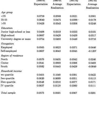
Table 1 compares nominal earnings expectations with realizations by demo­ graphic and household-income groups. In comparing expectations with reahza- tions, it must be stressed th at respondents report forecasts for the 1 2 months

following the day of the interview. Interviews were taken between May and July of 1990 for the 1989 survey, and between May and October 1992 for the 1991 survey, whereas income realizations refer to the calendar years 1989, 1991 and 1993. Thus I use as instrument the one-year forecast of income growth given in May-July 1990 for the growth rate of earnings between 1989 and 1991 and the one-year forecast of earnings given in May-October 1992 for the growth rate of earnings between 1991 and 1993. This imphes that expectations and reahzations do not coincide in time, and are not immediately comparable.

In an instrumental variables context, this is not a concern. AU th at is needed is th at the expectation be correlated with actual income growth and uncorrelated over time with the innovation term of the Euler equation (1). Under the nuU

hypothesis of the permanent income model, the latter condition is met. My approach is valid even if individuals underestimate or overpredict future income: all I need is that expected income growth helps predicting actual income growth. In the next section I show that income expectations are indeed strongly correlated with reahzations. Here I hmit myself to a descriptive analysis.

Only if incomes grew steadily over the two-year span one would expect subjec­ tive predictions to mirror half of the actual income growth rate. The last raw of

^^SHIW interviews usually start in May, with households asked about their income, assets

gind consumption of the previous calendar year. The reason is that previous experience has

shown that people report income more accurately when filing the income tax forms, which

Table 1 suggests th at while in 1990-91 expectations are quite close to reahzations

(5.7 against 5,2 percent), in 1992-93 expectations overpredict realizations (3.6 against 2 percent). Subjective expectations can be criticized because respon­ dents may not fuUy understand the survey questions: households with better education might therefore give more accurate income forecasts simply because they understand the survey questions better. However, individuals with less ed­ ucation do not appear to answer the survey questions less accurately than those with more. For instance, in 1989 individuals with junior high school or less re­ port an average expectation of 5 percent (vis-à-vis a reahzation of 5.5 percent), while individuals with coUege degrees overpredict income growth (7.5 percent vis-à-vis 5 percent). In 1991 it is the group with higher education th at makes better forecasts. One explanation of the discrepancy between expectations and realizations is the sharp and largely unanticipated 1993 recession. The explana­ tion usually offered for the recession was strong fiscal contraction and pension reform enacted by the Government in the Fall of 1992 (after the survey was com­ pleted), raising taxes, cutting pension benefits and increasing contributions. The recession had different effects for various population groups, hitting particularly the self-employed and the residents of the South. As will be seen, I wiU exploit knowledge of the groups that suffered mostly from the recession in modelhng the structure of the forecast error.

The pattern of expectations and realizations by population groups are also of interest. The young expect earnings to grow faster than the middle-aged and the elderly. Also employees predict their earnings growth more accurately than self- employed in both surveys. In part this is due to the fact th at the self-employed have greater income volatihty. Yet, comparison between subjective expectations and reahzations for the self-employed is difficult, because this group experienced an income decline of 12 percent in 1992-93, due to the 1993 recession and tax increases. Finally, expectations by income quartile do not indicate th at rich households predict earnings better that poor ones.

1992 (for 1993) of sophisticated econometric models and international institu­ tions. Respondents average expectation for 1990-91 (7.2 percent) comes closer to the realized value of 6 . 8 percent than OECD’s forecast for June 1990-June

1991 (5.4 percent). Results are reversed for the June 1992-June 1993 period; OECD projections are closer to realizations (4.2 percent and 4.8 percent, respec­ tively) ; while individuals overestimate the actual rate (with average expectations of 7.2 p e r c e n t ) . A n interesting feature is th at these average subjective infla­ tion expectations do not in fact mask a great number of implausible extreme values. More than 50 percent of the sample bunches the entire probabihty dis­ tribution for inflation between 5 and 7 percent. Finally, there is no clear pattern of subjective expectations by region, age, education or income.

3.2 Incom e risk

In the Euler equation it is the term (A InQ t+i — th at affects consumption growth. I assume that the only non-insurable risk faced by indi­ viduals is income risk, thus neglecting such other possibilities as rate of return and health risks. The subjective variance of the growth rate of real earnings is a f g = -f- — 2(f)(Ti^zTr- I have data on the marginal distributions of z and tt, but lack information on 0, the correlation coefficient between nominal earnings

shocks and inflation shocks. Thus in the empirical analysis I rely mainly on the subjective variance of the growth rate of nominal earnings {erf2) as my preferred proxy for expected consumption risk. One justiflcation for this choice is that it avoids arbitrary assumptions about the value of 0; furthermore, indexation

clauses in labor contracts often provide insurance against inflation increases. Only if utility is exponential and income is a random walk there is a one-to-one correspondence between income risk and consumption risk in the Euler equation (see chapter 1). Otherwise, the relation between the two is non-linear, depending

^®One possibility for the larger gap between expectations and realizations in 1992 is that

individuals were surprised by the implementation of income policies in July of 1992. These

income policies are generally thought to have been effective in reducing the actual inflation

rate. An alternative possibiHty is that consumers form adaptive expectations (in both 1989

on the utility function and the income process. For this reason one cannot give a structural interpretation of the estimated coefficients, i.e. in terms of prudence or underlying preference parameters. I am also aware that my measure of income risk is open to criticism. For instance, I rule out the potential effect of other non-insurable risks faced by households. And yet if income risk is poorly measured, or if income risk is only poorly correlated with consumption risk, one should find no statistical relation between consumption growth and the subjective variance of income.

4

S a m p le a n d s p e c ific a tio n is s u e

The panel component of the SHIW includes 1,137 households interviewed in 1989 and 1991, 2,420 households interviewed in 1991 and 1993, and 1,050 households interviewed in 1989, 1991, and 1993. Defining an “observation” as two years of data, this corresponds to 5,657 potential observations (2,187 in the 1989-91 panel, and 3,470 in the 1991-93 panel). I drop cases in which the house­ hold head changed (355 observations); those with inconsistent data on age, sex, or education (515 observations); those lacking data on subjective expectations (1,123 observations) ; and those lacking data for other variables used in the em­ pirical analysis (130 observations). The final sample therefore includes 3,534 “observations” (1,102 for 1989-91, and 2,432 for 1991-93). Since in most cases I have only one observation per household, I test primarily if the cross-sectional variation in consumption growth is explained by the cross-sectional variation in predicted income growth. I explain below how I deal with this problem.

As in previous studies, I control for individual preferences with age and change in family size.^® Testing for non-separabihties in the utility function is interesting in its own right and ensures that excess sensitivity does not arise from prefer­ ence mispecification. Given th at in my sample virtually no head is unemployed.

Given the wording of the questions, the probability of low income states, such as unem­

ployment, may not be reported.

also tried changes in other demographic variables, such as the number of adults or the

I introduce in the Euler equation the change in the employment status of the spouse. As mentioned, omitting labor supply indicators can bias upward the co­ efficient of expected income growth of the household head. The problem is not as serious than if I had total household earnings (employment is almost surely pos­ itively correlated with predicted income growth). However, the earnings of the head may still be correlated with the working spouse dummy because common macroeconomic shocks affect the probability of working and income prospects in the same direction. Other labor supply indicators - such as the change in the number of income recipients - were either not significantly different from zero or did not alter the results.

As mentioned, one should control for the structure of aggregate shocks, par­ ticularly in short panels. Even though forecast errors in consumption are unob­ servable, I do observe the cross-sectional pattern of income innovations. This can be used to extract potentially useful information about the structure of forecast errors in consumption, which depends on the income innovations.^® For instance, in the absence of common shocks, time dummies should not explain the forecast error. If instead macroeconomic shocks are important, time dummies will be correlated with the innovation in income and in consumption, and therefore can­ not be used as instruments to predict income. Rather, one should allow for time effects in the Euler equation.

Preliminary analysis indicates th at the income innovation (Alni/^t+i — is correlated not only with time dummies, but also with education, and dummies for occupation and region. Given the characteristics of the recessional episode of 1993, I find it plausible to assume that the forecast error contains an aggregate

^^Ektimating the elasticity of intertemporal substitution has proven to be extremely difficult

with panel data. Even in long panels - such as the PSID - the coefficient of the real interest rate

is often poorly determined or implausible. Initially, I constructed a measure of the

household-specific real interest rate, subtracting inflation expectations from the nominal rate on Treasury

bills. However, the coefficient of the elasticity of intertemporal substitution thus obtained was

not significantly different from zero and theoretically implausible. In the end, I decided to drop

the interest rate from the regressions: using two-year consumption changes with one-period

ahead inflation expectations, it is simply impossible to get the timing of the interest rate right.

component which is unevenly distributed across population groups and an id­ iosyncratic component th at averages out in the cross-section.^^ Tax increases for the self-employed or a stronger effect of the 1993 recession in the South would have such an eflFect (see also Miniaci and Weber, 1996). This implies th at group dummies (such as region and employment status) should not be used as excluded instruments to predict actual income growth.

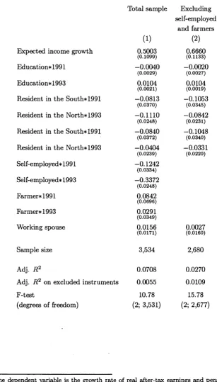
Table 3 reports the first-stage coefficients obtained by regressing actual income growth on expected income growth, time dummies, education, regional dummies and employment status interacted with year dummies, lagged employment status of the spouse, age, family size, and income risk. Overall, the first stage regression has good predictive power (the adjusted Fi? statistics is 0.07). The coefficient of expected income growth is 0.5 and significantly different from zero at the 1 percent level.^^ A conventional F-test on the excluded instruments (expected income and lagged employment status of the spouse) yields a p-value below 1

percent, confirming the validity of the instruments.

In the following section I thus present instrumental variable estimates of the following Euler equation:

A In Cit+i = OLiageu^i + Q2 -f ^-1 --yAwwif+i 4- /?Alnî/iÉ+i 4-

4-where F S a ^ i denotes family size, ^w w u+ i is the change in a dummy for spouse working full-time, denotes the expected variance as of time t of nominal in­ come growth, j the population groups affected by macroeconomic shocks, and 6j captures the effect of unevenly distributed aggregate shocks ^t+i on the forecast error in consumption.^^ In the empirical application I will also present estimates replacing predicted income growth F^itAlnpit+i with the subjective expectation

the empirical specification I thus assume that the forecast error in consumption growth

can be decomposed as Eu+x = 6jfxt+i + i/it+i,where uu+x denotes the idiosyncratic component.

^^Our instrument predicts well both income increases and income decreeises. The first stage

coefficients of expected income growth are, respectively, 0.45 and 0.64 in the samples expecting

positive and negative income growth.

^^My identifying assumption is therefore plim N~^ Kt+i = 0, where N is the number of

of income growth .

5

E u le r e q u a tio n e s tim a t e s

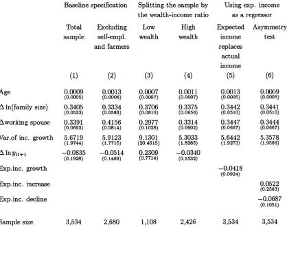
The results of estimating equation (2) are reported in column 1 of Table 4.

The coefficients of the demographic variables are well determined and have the “right” sign. The positive and significant coefficient of the change in the spouses employment status indicates th at expecting to work more in the future reduces current consumption. This will indeed be the case if leisure and consumption are non-separable. The coefficients of the group dummies are not reported for brevity.

The proxy for consumption risk is positive and significantly different from zero at the 1 percent level, and supports the theory of precautionary saving.

Since what I measure is not the expected variance of consumption but the ex­ pected variance of income growth, the coefficient has no structural interpretation. Nevertheless, its size (5.67) is most suggestive. W ith isoelastic utihty, prudence equals one plus relative risk aversion, and reasonable values for risk aversion vary between 1 and 1 0.

working wife and the variance of income growth does not affect the excess sen­ sitivity coefficient. Thus, in my sample there is no excess sensitivity even when the Euler equation is mispecified.

How should one interpret the role of group dummies and education in the Euler equation? Even though they were introduced as a device to eliminate the inconsistency of IV estimates in short panels, at least two other interpretations are possible. First, group dummies may account for preference shifts and for this reason should not be omitted from the Euler equation, otherwise income growth will simply proxy for the omitted variables (absent group dummies, excess sensi­ tivity is just a signal of misspecified preferences). The second possibility is that there is a subtler form of excess sensitivity, arising not from the correlation be­ tween consumption and income, but from the correlation between consumption and income predictors. To clarify this point, suppose th at (low) education, resi­ dence in the South and self-employment are predictors of the probability of being liquidity constrained in period t. If so, one may expect them to predict higher consumption growth between period t and t + 1. However, in the regressions of Table 4 the dummies for South and self-employment are negative, while the coefficient of education is positive (with the exception of the dummy for South in 1993, the other interaction terms are not statistically significant). While al­ ternative explanations for the effect of group dununies are therefore possible, I find it more plausible to attribute their role to the effect of unexpected aggregate shocks.