On M odelling th e Mass of Arctic
Sea Ice
Jennifer K aty H utchings
A thesis submitted in partial fulfillment
of the requirements for the degree of
Doctor of Philosophy of the University of London
Department of Space and Climate Physics
University College London
All rights reserved
INFORMATION TO ALL USERS
The quality of this reproduction is dependent upon the quality of the copy submitted.
In the unlikely event that the author did not send a complete manuscript and there are missing pages, these will be noted. Also, if material had to be removed,
a note will indicate the deletion.
uest.
ProQuest U642467
Published by ProQuest LLC(2015). Copyright of the Dissertation is held by the Author.
All rights reserved.
This work is protected against unauthorized copying under Title 17, United States Code. Microform Edition © ProQuest LLC.
ProQuest LLC
789 East Eisenhower Parkway P.O. Box 1346
A bstract
Sea ice has been highlighted as a chmate change indicator [IPCC, 1995], Models are
useful tools to study Arctic sea ice on decadal and longer time scales [Vinnikov et al.,
1999] and the viscous-plastic model has been identified as the best model available
to simulate ice motion [Kreyscher et a l, 2000],
Here we investigate whether a stand-alone viscous-plastic model reproduces ob
served ice thickness. The Kiel sea ice model and the UCL model, documented in this
thesis, are compared to ERS radar altimeter estimates of ice freeboard. Compared
to the observations, ice thickness is over estimated by 2 m in both models. Near
the Canadian Archipelago this thickness difference increases to 3 m. We investigate
whether a large thickness error in the model can be explained by errors in the model
force balance. A sensitivity study of ocean and wind drag coefficients and maximum
ice strength shows that the model ice thickness cannot be improved by only varying
the maximum ice strength.
The viscous-plastic model is computationally expensive to solve accurately, which
hinders its use in GCMs. We revise the numerical solution, introducing a new over
relaxation method which guarantees the stress solution is always within the yield
criterion. The convergence of the velocity vector is much improved compared to the
iterative scheme of Zhang & Hibler [1997]. Finally a numerical error is identified in
the traditional velocity correction scheme which accounts for up to 0.5 m of the model
ice thickness error. An efficient algorithm is designed and implemented to ensure the
fully coupled mass-momentum solution is found to numerical accuracy.
In this thesis we find that the viscous-plastic model over estimates Arctic ice
thickness in the late 1990s. Up to 25% of this error may be attributed to unresolved
mass-momentum coupling, and we suggest other errors may lie in thermodynamic
A cknow ledgem ents
First and foremost I would like to thank my supervisor, Seymour Laxon, for his sup
port, patience and good humour. Many thanks to Markus Harder, Duncan Wingham,
Neil Peacock, Jeff Ridley, Henry Weller and Harry Jasak for many helpful and en
lightening conversations. In particular I would like to thank Harry and Henry for
inspiration, guidance, tutorial and occasionally introducing interesting garden paths.
Thank you also to Danny Feltham for reading this manuscript, it is much appreciated.
1 Introduction 23
1.1 Sea Ice and The Climate ... 23
1.1.1 Thermohaline Circulation... 24
1.1.2 Ice Albedo Feedback ... 27
1.1.3 Sea Ice as a Climate Change Indicator ... 28
1.2 Observations of Arctic Sea Ice ... 29
1.2.1 Ice Area and Extent O b se rv a tio n s... 29
1.2.2 Ice Motion Observations ... 31
1.2.3 Ice Thickness O b serv atio n s... 31
1.3 Natural Variability... ... 33
1.4 O v e rv ie w ... 36
1.5 Thesis O u t l in e ... 38
2 M odelling Sea Ice 40 2.1 Conservation of Mass... ... 41
2.1.1 Ice T r a n s p o r t... 42
2.2 Conservation of M o m e n tu m ... 44
2.3 Constitutive L a w ... 45
2.3.1 Rheology ... 46
2.3.2 Viscous-Plastic Rheology ... 47
2.3.3 Ice S tre n g th ... 49
2.4 Model Param eters... 49
2.5 Determining Suitable Constitutive Models ... 50
2.6 Model V a lid a tio n ... 54
Contents 6
2.6.2 Parameter Tuning... 59
2.7 Numerical Modelling ... 60
2.8 Summary ... 62
3 Comparing A ltim eter Ice Thickness Estim ates and th e Kiel Sea Ice M odel 64 3.1 The Kiel Sea Ice M o d e l ... 64
3.2 Radar Altimeter Observed Ice th ic k n e s s... 67
3.2.1 Monthly Averaged RA Sea Ice Thickness ... 72
3.3 Comparing the Observed RA and Modelled Ice T h ic k n e s s... 75
3.4 Discussion ... 81
4 Num erical Solution o f the V iscou s-P lastic Sea Ice M odel 83 4.1 Finite Volume D isc re tisa tio n ... 83
4.1.1 Discretisation of Advection T erm s... 86
4.1.2 Interpolation Schemes ... 86
4.1.3 Discretisation of Diffusion T e r m s ... 89
4.1.4 Discretisation of Source T erm s... 90
4.1.5 Boundary C onditions... 90
4.1.6 Temporal D isc re tisa tio n ... 91
4.1.7 Discretisation of the Viscous-Plastic Model ... 93
4.2 Solution of the Linear System of E qu atio n s... 97
4.2.1 Matrix C o n d itio n in g ... 99
4.2.2 Convergence Rate for Solution of the Momentum Equation . . 100
4.3 Case S tudies... 104
4.3.1 Linear Viscous Test C a se ... 104
4.3.2 Two Dimensional Velocity Solution with Prescribed Ice Mass . 106 4.3.3 Example of Convergent/Divergent Flow ... 109
4.3.4 Example of Flow With a Wind V o r t e x ... 115
4.4 Summary ... 119
5 A Sim ulation o f Arctic Sea Ice 121 5.1 Modelling Arctic Ocean Sea I c e ... 121
5.2 Arctic Sea Ice Model R esults... 127
5.3 Comparison between Modelled and Observed Sea Ice Thickness . . . 132
5.3.1 Force Balance of the Arctic Sea Ice Model ... 134
5.4 Summary ... 141
6 Sensitivity o f Sim ulated Ice Thickness to Drag Coefficients and Ice Strength 144 6.1 I n tro d u c tio n ... 145
6.2 Thickness Error F u n c tio n ... 146
6.3 Sensitivity Analysis ... 147
6.3.1 Optimisation of the Drag Coefficients ... 147
6.3.2 Optimisation of the Maximum Ice Strength Parameter . . . 151
6.3.3 Sensitivity of the Thermodynamic Source T e r m s ... 156
6.4 Summary ... 159
7 A N ew Correction A lgorithm for the V iscous—P lastic Sea Ice M odel 161 7.1 In tro d u c tio n ... 161
7.2 Derivation of a Transport Equation for Ice S tre n g th ... 163
7.3 The p Correction A lg o rith m ... 165
7.3.1 Convergence Rate of the p Correction A lg o r ith m ... 167
7.4 One-dimensional Simulation of Ice C onvergence... 169
7.5 Arctic Sea Ice Simulation... 172
7.6 Summary ... 175
8 Summary and D iscussion 176 8.1 Summary of R e s u lts ... 177
8.2 Future D ire c tio n ... 179
List of Figures
2.1 The elliptical yield curve, with e — 2, normalised by P ... 47
3.1 Monthly mean modelled ice thickness, for May 1995... 66
3.2 Time series of mean ice thickness from the Kiel Sea Ice Model. . . . 67
3.3 Time series of monthly mean ULS ice thickness estimates, with open
water removed, and monthly mean RA ice thickness estimates. Re
produced with the permission of Neil Peacock... 68
3.4 Location of central points for SCICEX ULS comparison with RA
monthly mean ice thickness. Reproduced with the permission of Neil
Peacock... 70
3.5 Showing the correlation between submarine ULS mean ice thickness
and RA monthly mean ice thickness. Reproduced with the permission
of Neil Peacock... 71
3.6 Number of months when there are more that 100 individual thickness
estimates available per grid cell, during the ERS-1 mission... 73
3.7 RA monthly mean ice thickness gridded onto the model grid. May
1995... 74
3.8 The difference between modelled ice thickness and ERS-2 RA ice thick
ness estimates...*... 76
3.9 The regions for which monthly mean modelled and RA ice thickness
are compared. These are referred to as: (A) Pram Strait, (B) Canadian
3.10 Modelled and RA monthly mean ice thickness in the Pram Strait.
Monthly mean ice thickness estimated from draft measurements by
upward looking sonar (courtesy of the Norsk Polar Institute) are also
shown in orange. The model is shown in black, ERS-1 red and ERS-2
blue... 79
3.11 Modelled and RA monthly mean ice thickness above the Canadian
Archipelago. The model is shown in black, ERS-1 red and ERS-2 blue. 79
3.12 Modelled and RA monthly mean ice thickness in the Beaufort Sea.
The model is in shown black, ERS-1 red and ERS-2 blue... 80
3.13 Modelled and RA monthly mean ice thickness in the Nansen Basin.
The model is in shown black, ERS-1 red and ERS-2 blue... 80
3.14 Modelled and RA monthly mean ice thickness in the Laptev Sea. The
model is in shown black, ERS-1 red and ERS-2 blue... 81
4.1 A typical grid cell: Sa: is the face area vector for one cell face; d is the
distance between two neighbouring cell centres, p and n and U is the
ice velocity at p ... 85
4.2 Linear approximations of the integral of (j) over time: (a) the Euler Ex
plicit Method, (b) the Euler Implicit Method, (c) the Mid-point Rule
and (d) the IVapezium Rule. Modified from [Ferziger & Peric, 1997]. 93
4.3 The computational molecule for a transient-advective equation
discre-tised with Central Differencing on a two-dimensional square grid. . . 98
4.4 Velocity residual between iterations over the Momentum Equation,
discretised traditionally without matrix conditioning. The residual for
Ux is shown as a solid line, the dashed line is the residual for Uy. . . 102
4.5 Approach to convergent velocity solution with number of corrector
steps, with matrix conditioning. The residual for Ux is shown as a
solid line, the dashed line is the residual for Uy... 102
4.6 Approach to equilibrium of the stress state at one point. The stress
state is plotted at intervals of 15 iterations over the momentum equa
tion and equilibrium is reached to an acceptable tolerance within 20
List of Figures 10
4.7 The ice stress after 20 corrector steps, show in principal stress coordi
nates. Note that the solution falls within the yield curve... 103
4.8 Analytical solution of the linear-viscous system. There is no notable difference between the analytical and numerical solution when they are plotted together... 105
4.9 The difference between analytical and numerical solution of the linear- viscous s y s te m ... 105
4.10 Approach to equilibrium of the ar-component of ice velocity at the square centre for runs with time steps of 6 minutes and 1 hour. . . . 107
4.11 Equilibrium velocity field for the viscous-plastic model, with P* = 5000Nm-^... 107
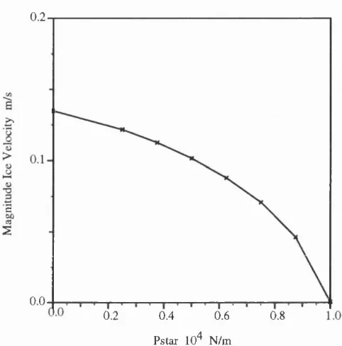
4.12 Central velocity for various values of P*... 108
4.13 Angle between free drift velocity and calculated velocity for various values of P* ... 108
4.14 Ice, initially 1 m thick, is blown across an ocean. We define the wind to blow in the or-direction. In time the ice converges towards the right coast, increasing ice thickness on the right of the domain and decreasing thickness on the left... 109
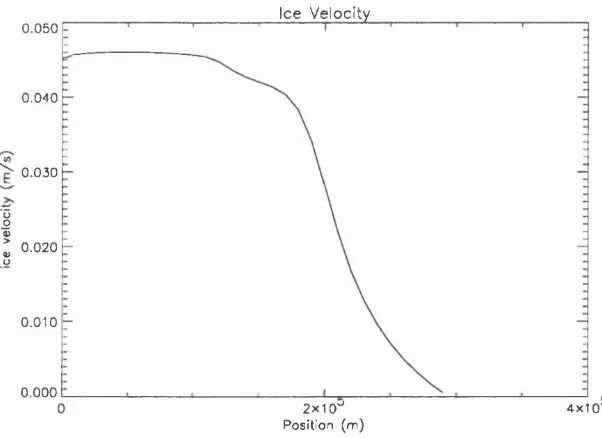
4.15 The approach of effective thickness to limiting values at various points along the lake... I l l 4.16 The approach of ice velocity to limiting values at various points along the lake... I l l 4.17 Ice thickness after one year integration, w i t h = 0.5 m... 112
4.18 Ice velocity after one year integration, with = 0.5 m... 112
4.19 Ice thickness after one year integration, with ho = 0.001 m... 113
4.20 Ice velocity after one year integration, with/lo = 0.001 m... 113
4.21 Ice thickness after 10 years of integration for various parameterisations of ice strength... 114
4.22 Effective ice thickness after 5 days, found with the particle-in-cell method. Reproduced with the permission of Greg Flato... 117
4.24 Effective ice thickness after 5 days. The transport equations discretised
with Central Differencing. The scale shows ice thickness (m)... 118
5.1 Grid of the Arctic Basin... 122
5.2 Mean sea surface topography, from 1992/1993 OCCAM run... 123
5.3 Typical 10m wind field, from NCEP/NCAR reanalysis, interpolated
onto the UCL model grid... 123
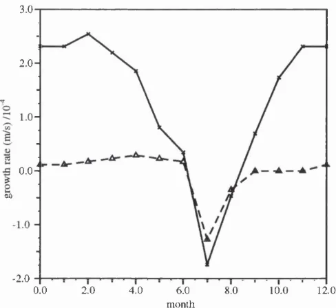
5.4 Growth rate of 0.5 m (solid line) and 4 m (dashed line) thick ice as a
function of time of year. Adapted from [Thorndike et al., 1975]. . . 124
5.5 Spin up of total ice mass for 1992. Time series are show for two
model runs, one initialised with zero ice mass and velocity, the other
initialised with h = Sm , A = 1 and zero velocity everywhere... 125
5.6 Time series of total ice mass on January for spin up of the twenty
year simulation... 126
5.7 Spin up of ice velocity at a point on January 1979. Both compo
nents of velocity are shown... 126
5.8 Modelled mean ice velocity for November 1996... 129
5.9 Arctic sea ice motion, field of interpolated mean ice motion. Found
from trajectories of automated buoys and drifting research stations
between 1893 and 1982 [Colony & Thorndike, 1984] 129
5.10 Modelled mean ice thickness for November 1996... 130
5.11 Climatology of winter ice thickness, from [Bourke & McLaren, 1992] 130
5.12 Time series of total ice area, 1979 until 1998... 131
5.13 Time series of total ice mass, 1979 until 1998... 131
5.14 The mean sea ice thickness difference between RA measurements and
UCL model for November 1996... 133
5.15 November 1996, monthly averaged force balance. The individual terms
are: Fa wind stress, ocean stress, Fi internal ice stress, Fc Coriolis
force and Ft force due to sea surface tilt. Note that the scale is different
in each sub-plot... 135
5.16 Points of interest for investigating the sea ice momentum balance.
Time series of the force balance at each point are shown in figs. (5.17)
List of Figures 12
5.17 Momentum balance at point 153 during 1996... 137
5.18 Momentum balance at point 230 during 1996... 138
5.19 Momentum balance at point 284 during 1996... 139
5.20 Momentum balance at point 392 during 1996... 140
5.21 Momentum balance at point 432 during 1996... 141
5.22 Momentum balance at point 70 during 1996... 142
6.1 The thickness error function. Contour plot of thickness error (sensi tivity), against drag coefficients, calculated for 1996... 148
6.2 Mean ice thickness in November 1996, modelled with various ocean and wind drag coefficients {Cw x 10“^ and Ca x 10“^)... 149
6.3 Mean ice velocity in November 1996, modelled with various ocean and wind drag coefficients [C^ x 10“^ and Ca x 10“^)... 150
6.4 The thickness error function, for 1996, calculated for simulations with various values of P*, Ca = 0.0016 and Cw — 0.0045... 152
6.5 The thickness error function, for 1996, calculated for simulations with various values of F*, Ca = 0.0003 and C^, = 0.0050... 152
6.6 Mean ice thickness and velocity fields, November 1996, modelled with P* = 5 X 10^,1 X lO'* and 1 x 10®Nm“ ^ The drag coefficients are Ca = 0.0012 and C^, — 0.0045. The ice thickness scale is enlarged in fig. 6.2... 153
6.7 Mean ice thickness and velocity fields, November 1996, modelled with P* = 5 X 10^, 1 X 10^ and 1 x 10^Nm“ h The drag coefficients are Ca = 0.0003 and C^ — 0.0055. The ice thickness scale is enlarged in fig. 6.2... 154
6.8 The thickness error function, calculated for 1996, for linear changes in thermodynamic ice growth/melt rate... 156
6.10 Mean ice thickness and velocity fields, for November 1996, modelled
with various thermodynamic growth/melt rates. The thermodynamic
rate of change of ice thickness is modified by a factor (0.25, 1 and
1.25). The ice thickness scale is enlarged in fig. 6.2... 158
7.1 The ice strength implicit successive correction scheme: an iterative so
lution procedure for the viscous-plastic sea ice model with p correction
steps... 166
7.2 Velocity residual against p correction step. The convergence of Ua, is
shown as a solid hne and \Jy as a dashed line... 167
7.3 Ice strength residual against p correction step... 168
7.4 Ice thickness after 10 years of integrations, with various values of the
P*... 169
7.5 Ice thickness after 10 years of integration, with P* = 5 x 10^Nm“ ^
and a minimum ice thickness ho = 0.001m. The solution obtained
with traditional correction steps is shown as a dashed line, the solution
obtained with p correction steps is shown as a solid line... 170
7.6 Thickness difference between two model runs after one year of inte
gration, run with traditional correction steps minus the run with p
correction steps... 171
7.7 Thickness diflFerence between two model runs after five years of inte
gration, run with traditional correction steps minus the run with p
correction steps... 172
7.8 Thickness difference between two model runs after ten years of inte
gration, run with traditional correction steps minus the run with P
correction steps... 173
7.9 Time series of total ice volume difference between the two simulations,
traditional correction algorithm minus p correction algorithm... 174
8.1 Grid of the Arctic Basin, embedded refinement is performed near
coastlines, capturing coastline detail... 177
A.l Difference between monthly averaged Kiel Sea Ice Model ice thickness
List of Figures 14
A.2 As fig. A.l,.for 1996... 183
A.3 Difference between monthly averaged Kiel Sea Ice model ice thickness
and ERS-2 RA ice thickness, for 1995 ... 184
A.4 As fig. A.3, for 1996 ... 185
A.5 As fig. A.3,.for 1997... 186
A.6 Difference between monthly averaged UCL Sea Ice model ice thickness
and ERS-2 RA ice thickness, for 1995... 187
A.7 As fig. A.6, for 1996... 188
2.1 Constants used in the standard simulation of Arctic sea ice... 50
4.1 Parameters used in simulation without transport, source: [Hibler,
N om enclature
Latin C haracters
A - ice area fraction
C - ice strength parameter
Ca - air drag coefficient
Cu; - water drag coefficient
F - thermodynamic growth rate
F - flux
Fl - lateral thermodynamic growth rate
i / - sea surface dynamic height
L - length of domain
M - number of months averaged over
N - number of grid cells with more that 100 RA thickness estimates
P - ice strength
P* - maximum ice strength
S - grid cell perimeter
Sa - source term in A transport equation
Sk - face length
a - discretisation coefficient
b - boundary index
c - linear water drag coefficient
d - distance between two adjacent cell centres
e - ratio of semi-major to semi-minor axes of an ellipse
/ - Coriolis force
g - acceleration due to gravity
g - ice thickness distribution function
h - ice thickness
ho - lower limit on ice thickness
halt - monthly mean RA thickness estimate
hmodei - monthly mean model thickness estimate
m - ice mass
p - ice strength normalised by pi
q - source
t - time
u - X component of ice velocity
V - y component of ice velocity
F - forcing terms in the momentum equation
I - identity matrix
M - matrix of discretisation coefficients
List of Tables 18
R - radius vector
S - grid cell perimeter vector
Sfc - face length vector
U - ice velocity
Ua - wind velocity
U«; - ocean current
k - unit vector normal to ice surface
n - unit vector perpendicular to grid cell face
r - residual
Greek Characters
A - second invariant part of stress tensor
r - diffusion coefficient
n - grid cell area
a - interpolation factor
T] - bulk viscosity
T]' - bulk viscosity normalised by pi
Pmax - limit on bulk viscosity
7 - UD-CD blending factor
/c - a factor
A - constant of proportionality
u - over-relaxation coefficient
(j) - yearly thickness error
ÿm - monthly thickness error
tp - compressibility
xp - ice thickness redistribution function
p a - air density
p i - ice density
p w - water density
Ta - air stress
- water stress
6a - air turning angle
Oy, - water turning angle
( - shear viscosity
- shear viscosity normalised by pi
Cmax - limit on shear viscosity
6 - velocity correction
€ - convergence error
£ - strain rate
(T - ice stress
Superscripts
- values at corrector step i
(f' - values at iteration n
- values at time t
List of Tables 20
Subscripts
Qb - value on the boundary face
Qk - value on the face
qn - value at neighbouring grid cell centre
Qp - value at grid cell centre
Qh - discretisation coefficient or source for h equation
qa - discretisation coefficient or source for A equation
Qu - discretisation coefficient or source for U equation
Qu - source for u equation
AIDJEX - Arctic Ice Dynamics Joint Experiment
AO - Arctic Oscillation
CD - Central Differencing
CG - Conjugate Gradient
DMSP - Defense Military Space Program
ERS - Earth Remote Sensing satellite
ESA - European Space Agency
ESMR - Electrically Scanning Microwave Radiometer
EVP - Elastic-Viscous-Plastic
F EM - Finite Element method
FVM - Finite Volume Method
G CM - Global Circulation Model / Global Climate Model
CD - Gamma Differencing
GFDL - Geophysical Fluid Dynamics Laboratory
GIN - Greenland-Iceland-Norwegian
GSA - Great Salinity Anomaly
HADCM2 - Hadley Centre Climate Model, version 2
List of Tables 22
ICCG - Incomplete Cholesky Conjugate Gradient
IPCC - Intergovernmental Panel on Climate Change
NAG - North Atlantic Oscillation
NCAR - National Center for Atmospheric Research
NCEP - National Center for Environmental Prediction
NO A A - National Oceanic and Atmospheric Administration
OCCAM - Ocean Circulation and Climate Advanced Model
PDF - Probability Density Function
PISO - Pressure Implicit Split Operator
RA - Radar Altimeter
SAR - Synthetic Aperture Radar
SCICEX - Scientific Ice Expeditions
SHEBA - Surface Heat and Energy Budget of the Arctic
SMMR - Scanning Multichannel Microwave Radiometer
SSM/I - Special Sensor Microwave/Imager
UCL - University College London
UD - Upwind Differencing
Introduction
Monitoring global climate change, addressing how it might impact mankind and as
sessing options for mitigating climate change is deemed important enough for the
creation of an Intergovernmental Panel on Climate Change (IPCC). This panel re
ports global mean increases in surface air temperature of 0.3^C to 0.6"C since the
19th century [IPCC, 1995]. The IPCC note that the non-linear nature of climate
hinders forecasting of future climate change, and improved representation of sea ice
in climate models is highlighted for further development. A well recognised method
of studying climate change is to investigate the transient response of global climate
models (GCMs) to carbon dioxide doubling scenarios. Such an experiment was re
ported in Manabe & Stouffer [1988], where it is predicted the largest atmospheric
temperature increases are in the Arctic during winter. They report a warming of
up to 15®C in this region, weakening of the thermohaline circulation in the North
Atlantic and reduction in sea ice mass. In similar experiments Stocker & Schmittner
[1997] found that the magnitude of thermohaline circulation weakening depends upon
the CO2 emission rate, and that the time to thermohaline collapse is dependent on
various model parameters.
1.1
Sea Ice and T he C lim ate
The polar regions play a significant role in the global circulation of the ocean and
atmosphere. They radiate and refiect more energy towards space than they absorb
and the energy deficit between the tropics and poles drives atmospheric circulation
1.1 Sea Ice and The Climate 2 4
freshwater input to the North Atlantic from the Arctic [Broecker, 1997]. It is well
known that GCMs indicate that the Arctic is a highly sensitive region to increases
in greenhouse gases [Cattle & Crossley, 1995]. To understand the extent to which
atmospheric warming might influence Arctic chmate and hence the global climate, an
understanding of Arctic and North Atlantic circulation and the polar energy balance
is required.
Sea ice is a key player in the Arctic climate system. It insulates the ocean from
the atmosphere and it contributes to radiative cooling, so that variations in ice cover
modify the Arctic heat budget. Sea ice export is the major source of fresh water in
the North Atlantic [Aagaard & Carmack, 1989], influencing global ocean circulation.
The two processes through which Arctic sea ice has been highlighted as influential
to global circulation are ice albedo feedback [Budyko, 1969] and fresh water export
through the Denmark Strait [Hakkinen, 1999].
1.1.1
T herm ohaline C irculation
The Arctic Ocean is stratified with an exceptionally fresh top mixing layer [Aagard
& Carmack, 1989]. Its temperature structure is unstable, with a surface layer that is
a few degrees colder than the bottom water. It is because the top water is fresh that
buoyancy is maintained, preventing deep convection.
The fresh Arctic surface layer is maintained by large river outflows and continen
tal runoff from Siberia and Canada [UNESCO, 1978, Aagaard & Carmack, 1989]. A
strong halocline prevents mixing of the surface water with warmer, more saline, denser
deeper water. Cooling the surface water to freezing point does not break down this
halocline. This is why perennial sea ice cover exists in the Arctic. If the warm deep
water was to mix with the surface water, more energy loss would be needed to cool the
ocean surface to freezing point than is possible through radiative and convective heat
loss, without a significant decrease in atmospheric temperature. It should be noted
th at continental runoff has large annual and interannual variability [Cattle, 1985],
which has implications for local maintenance of the halocline.
The freeze-thaw cycle of sea ice modifies the fresh water budget of the Arctic.
Brine rejection on freezing aids convective mixing. Melting in the summer releases
impor-tant implications for the circulation of the polar oceans [Aagaard & Carmack, 1989].
On the Siberian continental shelves brine rejection causes convective plumes under
freezing ice. Cold saline water runs off the continental shelf, descending to mix
with deeper Arctic water masses. In the Laptev Sea ice divergence, causing the
opening of leads throughout the freezing season, maintains this convective mixing
[Aagaard & Carmack, 1989].
Ice is constantly exported through the Pram Strait into the Greenland-Iceland-
Norwegian Sea. Vinje [1998] estimates the mean fresh water flux through the Pram
Strait is 2790km^yr"\ with considerable year to year variability of 13%. This vari
ability has been estimated with models: Walsh et al. [1985] show mean ice ex
port to be 1400km^yr"\ though they suggest the mean export is underestimated
and ice circulation is too slow in the model; Harder et al. [1998] find a seven year
mean Pram Strait export of 2700 km ^yr"\ with 21% interannual variability; Himler
et al. [1998] find a mean export into the Greenland-Iceland-Norwegian (GIN) sea of
3600 km^yr'L All studies find significant interannual variabilities, the magnitude of
which are in agreement with each other [Harder et al., 1998]. Himler et al. [1998]
note a large anomaly in their 40 year run; ice export in 1968 is found to be 50% larger
than mean export. This corresponds to the time period when the North Atlantic
surface water was observed to be anomalously fresh, the “Great Salinity Anomaly”
[Dickenson et al., 1988]. There is a large spread between model estimates of Pram
Strait export; Harder et al. [1998] demonstrates that this flux is sensitive to ocean
current, wind speed and air temperature. Unrealistic exports are predicted by Walsh
et al. [1985] and Harder et al. [1998] note that ice export is dependent on model con
figuration. To obtain the results outlined above Harder et al. [1998] tuned dynamic
parameters in the sea ice model with respect to drifting buoy speeds and ice thickness
observed at the North Pole.
Ice export through the Pram Strait is the main sink of Arctic sea ice [Thomas &
Rothrock, 1993], and is a major source of freshwater in the North Atlantic. In the
North Atlantic the saline surface water of the Gulf Stream meets cold fresh Arctic
water, causing overturning. The position of the polar front is controlled by the fresh
water influx to the North Atlantic, increased freshening causing overturning to occur
at more southerly latitudes. This overturning plays a key role in the global thermoha-
1.1 Sea Ice and The Climate 2 6
deep convection occurs, and the North Atlantic is thought to be a major source of the
global ocean’s bottom water. This ventilation is found to be sensitive to small changes
in the freshwater input to the Greenland-Iceland-Norwegian Sea [Rahmstorf, 1995].
Simulations of the meridional overturning cell in the North Atlantic demonstrate
the influence of sea ice export on the strength of overturning. It is found by Yang
& Neelin [1993] that feedbacks between oceanic poleward heat advection and sea ice
melting/freezing processes give rise to a self-sustained interdecadal oscillation in the
thermohaline circulation. Yang & Neelin obtained this result with a coupled thermo-
haline circulation, thermodynamic sea ice model. They later flnd a similar oscilla
tion in a three-dimensional ocean model coupled to a thermodynamic sea ice model
[Yang & Neelin, 1997]. The response of a thermohaline circulation model to pertur
bations in Norwegian Sea freshening was investigated by Rahmstorf [1994]. He found
th at an anomalously high, 4 year freshening of the Norwegian Sea does not cause
variability in the North Atlantic overturning and deep water formation; increased
freshening of the Norwegian Sea reduces overturning here, but this is balanced by
increased overturning in the Labrador Sea. The two circulation regimes identifled by
Rahmstorf [1994] are quite different, freshening leads to 5 K cooler sea surface temper
ature. Later interdecadal oscillations in the North Atlantic overturning were identified
in a three-dimensional ocean model [Rahmstorf, 1995]. Rahmstorf [1995] estimated
this overturning to be 20 Sv with variability of up to 3 Sv. Another study involving
a Atlantic-Arctic ocean model coupled with a thermodynamic-dynamic (viscous rhe-
ology) sea ice model shows that ice export significantly influences the strength of the
North Atlantic meridional overturning cell [Mauritzen &: Hakkinen, 1997]. It is found
th at increasing the mean ice export through the Fram Strait from 2000km^yr“ ^ to
2800km^yr“ ^ increases overturning by 2 to 3Sv per year. The time scale for ocean
adjustment to variation in ice export is estimated to be 5 to 10 years and it is de
duced that sea ice induced variability in overturning can reach 5 to 6Sv between
decades with anomalously low and high ice exports. The model’s response to short
time scale, anomalously large ice export events (e.g. 1000 km^ exiting the Denmark
Strait in 6 months) is investigated by Hakkinen [1999]. It was determined in a previ
ous model study [Hakkinen, 1993] that ice exports of this magnitude may be linked
to events such as the Great Salinity Anomaly. This export leads to a 20% change
to take several years. The ice exports considered in these experiments are indicative
of observed natural variability. Model experiments show a clear link between North
Atlantic overturning and sea ice export.
Quantifying the ventilation of the deep ocean is essential to our understanding of
the role the ocean plays in the E arth’s climate. Modelling studies indicate that atmo
spheric decadal variability might be transfered to the ocean through a sea ice mecha
nism. Current understanding is that atmospheric variability may cause decadal vari
ability in ice export through the Pram Strait [Proshutinsky & Johnson, 1997], which
is turn may modulate overturning in the the North Atlantic. Determining the magni
tude of North Atlantic overturning and how this is modulated by ice export through
the Pram Strait and Denmark Strait may provide insight into possible climate change
scenarios [Broecker, 1997]. Hydro-graphic data in the northern North Atlantic show
variations in outflow from the Nordic Seas to the deep Atlantic Ocean, flow doubling
and then returning to previous values over the last four decades [Bacon, 1998]. Bacon
suggests this variability may be forced by variability in polar air temperature which
in turn may be connected to recently observed polar warming [Rigor et al., 1999].
Investigations of the mechanism controlling decadal variability of the thermohaline
circulation would be complemented by improved estimates of sea ice flux through
the Pram Strait. Models are the only means of studying this export over time scales
greater than a few decades. Hence we must be confident that these models correctly
reproduce ice circulation and mass.
1.1.2
Ice A lb ed o Feedback
Sea ice and the atmosphere are predominantly coupled through ice albedo feedback.
Ice is more reflective to short wave radiation than the ocean, ice having a higher
albedo, hence the creation of sea ice amplifies polar atmospheric cooling. Conversely
ice melt enhances atmospheric warming. Excessive warming of the polar regions,
leading to ice melt could enhance global warming [Mitchell, 1989]. It is believe that
the influence of albedo feedback is not straight forward; the effect of increased cloud
cover and ocean surface freshening are probably important [Walsh, 1991].
As the climate is a complex non-linear system, GCMs are relied upon to investi
1.1 Sea Ice and The Climate 2 8
use crude grid box average parameterisations of albedo. It is common practice to tune
albedo to optimise atmospheric simulation, see for example [Manabe & Stouffer, 1980,
Washington & Meehl, 1983]. This tuning is unphysical and may mask systematic er
rors in the model [Shine & Henderson-Sellers, 1985]. It has been found that changing
albedo parameterisation in GCMs leads to differing climate sensitivity and modified
global atmospheric circulation [Meehl & Washington, 1990].
Sea ice in GCMs is often modelled thermodynamically as a uniform slab without
leads, with albedo linearly dependent on surface temperature and accounting for sur
face melt and snow cover [Manabe & Stouffer, 1988, Mitchell etal, 1987, Wilson &
Mitchell, 1987]. Albedo feedback is found to vary between 0.16 and 0.7Wm“ ^K“ ^
depending on the method used to represent albedo feedback [Ingram et al., 1989]. In
creasing albedo feedback, by decreasing sea ice sensitivity to melt, has been shown to
have profound influence on low frequency variability in a model atmosphere [Meehl
et ah, 2000].
Kreyscher et al. [1997] flnd that ice dynamics used in GCMs - typically free
drift with stoppage when ice becomes thick - is poor at representing ice motion
and area. Model ice cover is sensitive to the energy balance at the ice-atmosphere
interface and ice dynamics [Lemke et ah, 1997]. Lemke et al. flnd th at using more
realistic ice dynamics (including a viscous-plastic rheology) decreases the modelled
sea ice sensitivity to atmospheric perturbations. This indicates that determination
of the magnitude of ice albedo feedback could be aided by including realistic models
of sea ice cover within GCMs [Ingram et ah, 1989]. Sea ice has been highlighted
[IPCC, 1995] as one of the more uncertain processes in GCMs, and the IPCC calls
for the development of improved sea ice models for chmate studies.
1.1.3
Sea Ice as a C lim ate Change Indicator
It is thought that changes in Arctic sea ice extent might be an early indicator of
global warming [ACSYS, 1992, Budd, 1975]. Through ice albedo feedback, the ice
extent is sensitive to atmospheric warming. An increase in temperature, leading to
ice melt, will be amplified as less short wave radiation is reflected back to space, in
creasing ice melt. Similarly, a reduction in the freshwater input to the Arctic may
[Aagaard & Carmack, 1989]. COM experiments show that in response to increased
greenhouse gases (i.e. doubling atmospheric CO2) Arctic sea ice substantially de
creases in extent [Cattle & Crossley, 1995, Manabe & Stouffer, 1988]. The accuracy
of these global warming predictions are uncertain, see for example the criticism of
Walsh [1991]. In the next section we outline observed trends in Arctic sea ice and
discuss their indication of climate change in the Arctic.
1.2
O bservations o f A rctic Sea Ice
The Arctic is an inaccessible, hostile ocean. Until the later half of the 20th Century
the study of global ice motion and mass balance was infeasible. Fishing and whaling
vessels have been navigating the Greenland-Iceland-Norwegian Sea since the 1600s,
though their mapping of the ice edge is erratic. In-situ records of the ice edge are
considered to be reliable from 1953 onwards [Walsh & Johnson, 1979]. More detailed,
and consistent, observations of the global ice circulation and distribution have become
available relatively recently. Rehable records of ice drift, coverage and thickness in
the central Arctic begin in the late 1960s. Since then operational monitoring of the
ice state, in particular satellite monitoring of sea ice coverage, has become routine.
There are still gaps in this monitoring, and until recently ice thickness information
was sparse. Ice thickness data has recently been determined by satellite altimetry
[Peacock, 1999] and continuous, winter time data for most of the Arctic exists from
1993 onwards. Fluxes in the Arctic sea ice were inferred from a handful of cruises,
moored buoys, drifting buoys and manned ice stations, though with recent advances
in satellite monitoring of ice velocity these fluxes may be inferred more accurately
than previously possible.
1.2.1
Ice A rea and E xten t O bservations
Ice coverage has been monitored routinely since the 1950s [Mysak Sz Manak, 1989].
Since 1973, when the EMSR was launched, space-borne microwave radiometers have
been used to study sea ice cover [Zwally et al., 1983]. Sea ice extent, the total ice area
including open water within the pack, is mapped and areal fraction of ice monitored.
There are various algorithms to extract this information from observed brightness
1.2 Observations of Arctic Sea Ice 3 0
and the GSFC Bootstrap algorithm. For a comprehensive review of sea ice analysis
with passive microwave algorithms see [Steffen et al., 1992]. The SMMR and SSM/I
instruments aboard the NOAA/DMSP series of satellites provide constant monitoring
from October 1978 onwards.
Analysis of the passive microwave record of sea ice extent from 1978 until 1988
indicates a 2% decline in Arctic sea ice extent (with statistical confidence 96%)
[Gloersen & Campbell, 1988]. After analysis of the extended SMMR and SSM/I
record Johannessen et al. [1995] suggest there has been a significant decrease in
sea ice extent of 3% per decade since 1978. A much longer record of sea ice extent,
from in-situ observations of the ice edge since 1953, has been analysed by Mysak
& Manak [1989] who find the time of the Great Salinity Anomaly corresponds to
increased ice extent. Updated versions of this data set show no long term trends
[Barry et al., 1993]. Trends observed in the passive microwave sea ice record do not
conclusively show an overall decrease in total ice extent compared to interannual vari
ability. Passive microwave sea ice observations can be classified as multi-year or first
year ice [Steffen et al., 1992]. Trends in the area of multi-year ice were investigated
by Johannessen et al. [1999] and it was found to have decreased by 14% since 1978.
Although the trend in total Arctic ice cover is small, it is curious that there is such a
large trend in multi-year ice. This loss of multi-year ice could be evidence of transition
between different regimes of the Arctic sea ice cover. Johannessen et al. [1999] note
th at the more pronounced decrease in multi-year ice area is from 1987 onwards and
could be associated with changes in atmospheric circulation.
Differences in interannual variability between regions is apparent in the ice ex
tent record. In the Greenland Sea the ice edge position varies considerably, and
decadal time scale variations are found to correlate to anomalous salinity events in
the North Atlantic [Mysak & Manak, 1989]. Regional interannual variations in ice
area are outlined in [Parkinson & Cavalieri, 1989]. Summer ice extent in the Cen
tral Arctic shows variability between years with anomalies of up to 20% of the to
tal ice cover [Parkinson, 1991]. Over the last three years, 1996-1999, the summer
ice extent has been consistently smaller than average, with ice receding above 82^N
in the Barents Sea in August. The lowest ice extent on record occurred in 1998
1.2.2
Ice M otion O bservations
Routine monitoring of the sea ice motion began in the 1950s. The mean ice motion
has been determined from the drift of ice camps and buoys. Mean seasonal velocity
fields for 1979 onwards, from the International Arctic Buoy Program (lABP), are pre
sented in [Colony & Thorndike, 1984]. The main features of the mean motion are a
clockwise gyre in the Beaufort Sea and the Transpolar Drift running from the Siberian
coast through the Fram Strait. The time for ice to make one complete circuit of the
Beaufort gyre is 5 to 10 years. Ice traverses the Transpolar Drift Stream, accelerating
towards the Fram Strait, in about 3 years [Thorndike, 1986]. Over yearly time scales
the ice drift reflects the roughly equal influence of wind and ocean surface currents.
On shorter, daily time scales a strong relationship is found between ice velocity and
geostrophic wind. There is considerable monthly variability, and interannual variabil
ity, in the ice drift [Thorndike & Colony, 1982].
Other ice velocity data sets exist. Synthetic Aperture Radar (SAR) provides local
ice velocity fields at much finer resolutions than buoy data [Fily & Rothrock, 1986,
Kwok et al., 1990]. More recently ice velocity has been derived from passive mi
crowave radiometry. The SSM/I instruments aboard the NOAA/DMSP series of
satellites are routinely used to monitor ice coverage. Algorithms have been devel
oped to estimate ice velocity with brightness temperature cross correlation techniques
[Kwok et ah, 1998]. This data provides good coverage in the winter, resolving veloci
ties over 3 day time scales. Ice velocity fields found by optimal interpolation of lABP
Buoy drifts have a spatial resolution of hundreds of kilometres. It is expected SSM/I
ice velocities will provide more accurate and detailed ice flux analysis than obtained
with lABP velocity fields [Thomas & Rothrock, 1993]. Areal fluxes of ice through the
Fram Strait, and from several other regions, have been determined by combination of
SSM/I velocity and concentration [Martin & Augstein, 2000].
1.2.3
Ice T hickness O bservations
In order to determine sea ice mass we require observations of ice thickness. Until
recently there was little ice thickness data available, the main data sets being Upward
Looking Sonar (ULS) measurements of ice draft. ULS are moored in several locations
1.2 Observations of Arctic Sea Ice 3 2
[Vinje et a l, 1998]. Submarine cruises provide more extensive ULS coverage in the
Arctic and Greenland Sea. Declassified data from US Navy cruises provide the only
ice thickness measurements th at large scale sea ice models have been verified against.
A climatology of ice thickness, produced from 12 cruises between 1958 and 1987,
is presented by Bourke & McLaren [1992]. Sea ice thickness is highly variable on
horizontal scales of tens of metres to kilometres. There is a gradient in mean ice
thickness across the Arctic Basin, reflecting ice convergence towards the Canadian
Archipelago. The seasonal cycle in ice thickness was identified, with mean ice thickness
varying by a metre. The largest values of mean ice thickness, over 7 m, occur along
the Canadian Coast. Thinner ice, up to 3 m thick, is found in the Beaufort Sea. The
Bourke & McLaren [1992] climatology is limited to a box in the Canadian side of the
Arctic, encompassing part of the Eurasian Basin and Beaufort Sea.
There have been attempts to deduce trends in ice thickness between submarine
cruises. The variability of ice thickness measured during the twelve cruise included in
the Bourke & McLaren [1992] climatology is investigated by McLaren et al. [1994].
Only around the north pole was there sufficient data for analysis of interannual vari
ability. Mean ice thickness here was found to be 3.6 m with year-to-year variabilities
of 0.8 m. This large interannual variability obscures detection of climatic trends in ice
thickness. Ice thickness along a section of the Eurasian Basin on two cruises in 1976
and 1987 was analysed by Wadhams [1995]. A mean decrease in ice thickness between
the two cruises was reported. Both cruises sampled ice at different times of year, for
differing tracks and only two time periods were sampled, hence it is tenuous to draw
conclusions about large scale trends in ice thickness from this data. Wadhams ad
dressed this criticism in [Wadhams, 1997], claiming that statistically significant trends
could not be found around the north pole but that the difference in area averaged
thickness in the Eurasian Basin is statistically significant.
In the late 1990s the SCICEX (Scientific Ice Expeditions) project was instigated.
Submarine ULS data was collected in a region of the central Arctic encompassing the
Beaufort Sea and North Pole. Data is available from 6 cruises in 1992, 1993 1996 and
1997. This data has been analysed and compared to submarine ULS data collected
between 1958 and 1976. Based on comparisons at 24 coincident points, of a mainly
Autumnal data set, it is identified that mean ice thickness has decreased from 3.1 m
et al. [1999] report that ice volume in the Arctic has decreased by 40% over this time
period.
During the SHEBA (Surface Heat and Energy Budget of the Arctic) cruise, 1997,
ice thicknesses in the Beaufort Sea were found to be thinner than expected from
climatology [McPhee et al., 1998]. The mean ice thickness was reported to be about
1.5m. It can not be determined whether this was a local anomaly due to shifting
circulation patterns or freshwater influx to the region. This result does support the
general consensus that, on average, ice in the whole Arctic was thinner in the late
1990’s than has ever previously been recorded.
In 1997 the first direct measurements of ice freeboard were made with a satellite
altimeter [Peacock, 1999]. Ice freeboard has been mapped during the ERS-1 and ERS-
2 missions, from May 1993 onwards. This dataset is discussed below in section 3.2
and has been shown to be in good agreement with the SCICEX data.
To summarise, it is well documented that sea ice in the late 1990s is thinner and
less extensive th at previously observed. Consistent and rehable records of ice extent
only exist since the late 1970s. Records of ice thickness are sparse, and synoptic
satellite altimetry observations over the whole Arctic are available for less than a
decade. These time scales are too short to determine climatic trends in Arctic ice
cover. To understand whether the observed decrease in ice mass is a climate change
signal we require knowledge of the interannual and decadal variability of sea ice mass,
and how this is related to atmospheric and oceanic variability. At present, models
are the only means of studying sea ice variability throughout this century. These
could be used in conjuction with thickness observations from the last three decades
to understand whether the observed decrease in ice thickness is part of a long time
scale Arctic sea ice cycle.
1.3
N atural V ariability
Decadal scale variability of the ice cover has been observed in the passive microwave
record [Gloersen & Campbel, 19191, Gloersen & Campbell, 1988, Parkinson, 1991,
Parkinson & Cavalieri, 1989]. Anomalies in sea ice extent are found to be corre
lated to low frequency atmospheric variability [Gloersen, 1995]. Interannual sea ice
1.3 Natural Variability 3 4
with fields from atmospheric analysis produced with global numerical weather pre
diction models, show considerable interannual variability in ice circulation and mass
[Walsh et ah, 1985, Himler et ah, 1998]. A single column energy balance model, only
accounting for sea ice thermodynamic and coupling to the atmosphere, predicts that
ice mass varies on predominantly decadal time scales [Bitz et al., 1996]. Given the
variability apparent in their model Bitz et al. estimate the length of time ice thickness
must be monitored in order to determine a climate trend. Based on sea ice thickness
having a 15 year characteristic time scale with a variance of 0.75 m, they estimate
that 60 years of monitoring are required before a 1.4 m observed trend is significant at
95% confidence. Over a 30 year time period an observed trend of 0.7 m has only 70%
confidence. This highlights why we need to estimate the natural climate variability
of sea ice before the observed decrease in Arctic ice mass [Rothrock et al., 1999] may
be understood.
Sea ice trends have been examined with GCMs, where greenhouse warming experi
ments project that increasing atmospheric warming will lead to a decrease in Northern
Hemisphere sea ice extent [Manabe & Stouffer, 1988]. More recently Vinnikov et al.
[1999] examine the response of sea ice extent in two GCMs. The two models considered
are: (1) the GFDL model (R15) which represents sea ice thermodynamically without
accounting for the evolution of leads and (2) the Hadley Centre model (HADCM2)
representing ice thermodynamically with lead parameterisation; both allow ice to be
advected by ocean currents. Both models show similar ice extent trends over cen
tennial time scales, even though HADCM2 underestimates sea ice extent. Vinnikov
et al. [1999] assess the significance of these trends to determine whether they are the
result of natural variability in the model system. They find very low probability that
modelled and passive microwave observed trends are the result of random variation,
suggesting the trends are related to anthropogenic global warming. This result relies
on the models’ natural variability reproducing th at observed in nature. However there
is no reliable evidence that GCMs correctly represent atmospheric-ice coupling. The
assumption that small scale processes can be separated from large scale circulation,
so long as small scale parameterisation results in realistic circulation and overall vari
ability, is suspect [Shackley et al., 1998]. Further verification of modelled coupling
between ice, atmosphere and ocean is required; toward this end we need improved
In a model study Proshutinsky & Johnson [1997] found two modes of wind driven
ice circulation in the Arctic Ocean. The two regimes are referred to as cyclonic and
anti-cyclonic. Cyclonic circulation results in an enlarged Beaufort Gyre and shifting
of the Transpolar Drift towards the Siberian Coast, transporting ice from the Laptev,
East Siberian and Chukchi Seas. Anti-cyclonic circulation has a weakened Beaufort
Gyre and the Transpolar drift is shifted into the Central Arctic. Both circulation
patterns are associated with changes in oceanic circulation, the cyclonic regime hav
ing fresher surface water and stronger vertical stratification than the anti-cyclonic
regime. Coupled ice-ocean model results suggest that the regimes alternate and may
be persistent for 5 to 7 years [Proshutinsky & Johnson, 1997]. Shifts between regimes
are forced by changes in the location and intensity of the Icelandic atmospheric low
and the Siberian atmospheric high. It is possible th at the Proshutinsky & Johnson
model of atmospheric control of Arctic ice could explain some of the observed Arc
tic ice mass variability. Decadal time scale oscillations in atmospheric low pressure
systems in the Arctic and North Atlantic are well documented and linked to the
NAO, first described by Sir Gilbert Walker in 1930, and the Arctic Oscillation (AO)
[Thomas & Wallace, 1998]. Recently the NAO and AO has been linked to sea ice
extent variability [Feng & Wallace, 1994, Mysak & Veneges, 1998]. Feng and Wallace
[1994] identify that temporal variability in sea ice extent is strongly coupled to the
NAO, the atmosphere leading the ice extent by 2 weeks. The influence of the atmo
sphere is found to be strong enough to halt climatological advance of the ice edge
in some regions, enhancing it in others, for example a see-saw in sea ice extent be
tween the Labrador and Greenland Seas. They indicate that local wind stress and
thermodynamic forcing can explain sea ice variability in most regions; except in the
Greenland Sea. Mysak & Veneges [1998] performed principle component analysis on
40 years of ice concentration and sea level pressure data. They found that a standing
oscillation in sea level pressure, characterised as the AO, is correlated to a cyclic os
cillation in sea ice extent. More recently Wang & Ikeda [2000] analyse data from 1901
to 1995 and find that 41% of the variance in sea ice extent can be explained by the
AO. The second mode apparent in the sea ice extent record is related to the NAO, as
sea ice anomalies in the Labrador and Greenland Seas are out of phase.
In the late 1990s Arctic atmospheric circulation was in the NAO and AO phases
Proshutinsky-1.4 Overview 3 6
Johnson model [Wang & Ikeda, 2000]. It is thought the observed decrease in ice mass
in the late 1990s may be linked to increased cyclonic ice circulation. Maslanik et al.
[1999] suggest reduced ice extent in the Summer of 1998 was preconditioned by light ice
cover in Autumn 1997 and decreased northerly winds causing a reduced Beaufort Gyre
in Winter 1998. During SHEBA (October 1997) increased freshening of surface water
and thinning of sea ice were observed, compared to AID JEX (1975) measurements
[McPhee et al., 1998]. The SHEBA site was located near the centre of the Beaufort
Gyre, where historically the thickest perennial sea ice has been recorded. Near this
site hydro-graphic surveys from 1987 onwards indicate th at the freshening observed
in 1997 was Mackenzie River outflow [MacDonald et al., 1999]. Fresh water from ice
melt was recorded in the early 1990s indicating a reduction in ice thickness from 6 to 4
metres [MacDonald et al., 1999]. This ice melt corresponds to atmospheric circulation
becoming more cyclonic. It is suggested that increased ice melt was in response to this
shift in circulation regime. Hydro-graphic surveys from SCICEX cruises indicate that
the mid-Eurasian Basin surface waters were remarkably saline during the 1990s, with
the cold halocline layer retreating from the Eurasian Basin [Steele & Boyd, 1998]. An
expected consequence is increased heat flux from the deep Atlantic Water layer to the
surface layer. At the moment it is unclear whether these observed conditions are due
to a stable decadal Arctic circulation cycle or whether the conditions will persist,
resulting in loss of perennial ice in the Arctic.
1.4
Overview
To understand recent observations that the Arctic sea ice thickness and extent is
decreasing, the interannual and decadal variability of ice mass must be determined.
Arctic wide monitoring of ice coverage and ice velocity, obtained from satellite borne
passive microwave radiometers, is available from 1978 onwards. Synoptic observa
tions of ice thickness have become available recently, radar altimeter data is avail
able from 1993 onwards. Future missions are planned (Cryosat, ENVISAT and
Icesat) which will extend the altimeter ice thickness record beyond the lifetime of
ERS. All other ice thickness data sets are sparse and do not have long temporal
coverage. Trends have been determined in sea ice records: ice extent is observed
Johannessen et a l, 1995]; ice thickness has decreased by 40% since the 1970s in sub
marine records [Rothrock et al., 1999]. Unfortunately, as these records are rather
short, it can not be identified whether these trends are due to climatic or shorter
term (decadal) variability. At present models are used to study long time scale sea
ice variability and trends.
It is well documented that sea ice plays an important role in global climate. In
models used to study climate change sea ice is treated rather simplistically. These cli
mate models have been found to be sensitive to the treatment of sea ice [Ingram, 1989].
If we are to trust climate model results, it is important that the representation of sea
ice is accurate. The ice cover must realistically modulate fluxes between the ocean
and atmosphere. The extent of the ice, leads and thin ice must be well represented;
this is controlled by ice dynamics as well as thermodynamics [Lemke et al., 1997]. Sea
ice also influences the global ocean circulation, through export of fresh water into the
North Atlantic. In order to correctly represent this flux Arctic sea ice mass must be
correctly modelled. To understand how interactions between atmosphere, ice, ocean
and atmospheric oscillations control Arctic sea ice mass further process studies are
required. It is desirable to use models to determine the dominant periods of sea ice
variability, and whether ice mass variability may be linked to known atmospheric
variability. It may be possible to use climate models to investigate variability of sea
ice mass and how this influences ocean circulation.
Sea ice models used in GCMs do not represent Arctic ice mass correctly. Indeed,
there is some concern th at their misrepresentation of sea ice casts doubt on Arctic
trends identifled in climate warming scenarios; it has been shown that dynamic-
thermodynamic sea ice models with plastic rheology are required to provide cor
rect fields of sensible heat, latent heat and salt flux to the atmosphere and ocean
[Lemke et al., 1997]. Stand alone sea ice models and coupled ice-ocean models are
being used to study interannual variability, for example ice mass flux through the
Pram Strait has been modelled and correlation between this and anomalous salinity
in the North Atlantic has been identifled [Hakkinen, 1995]. In these studies we must
have confidence in the tool used; it is important to verify that the sea ice model