Flow characteristics of control valve for different strokes

Flow characteristics of control valve for different strokes

Jana Jablonská1,a and Milada Kozubková1

1_{VŠB-Technical University of Ostrava, Faculty of Mechanical Engineering, Department of Hydromechanics and Hydraulic Equipment,} 17. listopadu 15/2172, 708 33 Ostrava – Poruba, Czech Republic

Abstract.The article deals with the determination of flow characteristics and loss coefficients of control valve when the water flows in the interval of operating parameters, including the evaluation of vapour and air cavitation regime. The characteristics of the control valve are measured on the experimental equipment and subsequently loss coefficients are determined. Data from experimental measurements are used for creating of mathematical model with vapour and air cavitation and verification results. This validation will enable the application of methods of numerical modelling for valves of atypical dimensions e.g. for use in nuclear power industry. The correct knowledge of the valve characteristics and fundamental coefficients (e.g. flow coefficient, cavitation coefficient and loss coefficient) is necessarily required primarily for designers of pipe networks.

1 Cavitation in control valves

Hydrodynamic cavitation appears in hydraulic armatures during their current operation. This phenomenon is discovered for example in the narrowest gap between the regulating cone and the valve body. At this location the liquid is accelerated and the pressure is decreased. Vapour bubbles are formed in the liquid from cavitation nuclei (undissolved air and impurities). Growth of cavitation nuclei begins when the pressure falls below the value of saturation vapour pressure. It causes a sudden production of vapour bubbles, which are abducted by the liquid. Recover increase of pressure occurs behind the place of the smallest cross section. Vapour bubbles suddenly are diminished and disappeared by influence of the pressure. The gases contained in the bubbles partially diffuse into the surrounding liquid which is penetrated in their place. The remnants of gases in place of disappearing bubbles repeatedly decrease and increase their volume due to compressibility [1, 5]. Cavitation is influenced not only by vapour but also by dissolved air in the water, which is released at the narrowest section of the valve or by undissolved air sucked into the hydraulic circuit. In terms of the dynamics of bubbles it behaves like vapour. The maximum volume of the dissolved air in the water is 2% at normal conditions [3, 14, 15].

Cavitation in control valves is characterized by vibrations. Sound similar to the intermittent crackle in the field of the audible frequency can be observed in many cases [2, 4]. The occurrence of cavitation cloud in the flow field significantly influences the flow parameters of the valve [3, 5].

2 Mathematical models

Cavitation model assumes a minimum of two-phase mixture flowing - water and vapour. The release of dissolved air occurs at higher Reynolds numbers, and therefore model with three phases - water, vapour and air is considered. The dynamics of the gas comes from Rayleigh - Plesset equation for the dynamics of bubbles

( )

( )

for certain value of local far pressure p∞(t) the bubble radius Rb(t) can be determined; pvap is bubble surface

pressure; σ is surface tension; νl is kinematic viscosity of

liquid; l is density of liquid; see [9, 10, 11].

Transport equation of vapour volume fraction is taken into account.

(

)

(

)

t ¸_¹=∇ ∇ + −

· ¨ © § ∇ + ∂ ∂ → γ ρ ρ (2)

where fvap is volume fraction of vapour; u is the velocity

vector of the mixture; is density of the mixture; Re is

efficient exchange factor for p < pvap; Rc is efficient

exchange factor for p > pvap.

Individual cavitation models are different at the determination of Re and Rc. For Schnerr Sauer cavitation

model the follows equations are valid vap p p≤ ( ) l b vap l e p p R R ρ α α ρ ρ ρ ₋ − = vap 3 2 3 1 (3) vap p p≥ ( ) l b vap l c p p R R ρ α α ρ ρ ρ vap 3 2 3

1− −

= (4)

C

Numerical simulation of flow in the valve is based on solution of Navier-Stokes equations by finite volume method and is performed by software Ansys Fluent 15. Model k- RNG has been used for modelling. This model is one of the modifications of the basic k- standard model. It is derived from the Navier-Stokes equations, using a mathematical technique called “renormalization group” (RNG) method. The model increases the calculating accuracy for the turbulent flow of lower Reynolds numbers and primarily for vortex flow. Therefore it is more reliable.

3 Description of the experiment

To test the control valve, a test circuit was built according to SN EN 60534-2-3 [6]. The test circuit is on figure 1.

Figure 1. Circuit scheme – 1 - tank, 2 – pump, 3 – pump

frequency converter, 4 – setting valve at inlet, 5 – frame, 6 – flowmeter, 7 – sampling point of pressure at inlet, 8 – test flow control valve DN40, 9 – sampling point of pressure at outlet, 10 – setting valve at outlet.

Measured element is the valve with a modified cone. The cone is adapted to be armature with control capabilities.

For measurement the water was used, i.e. an incompressible medium at a temperature of 20 °C. Accurate determination of the cone stroke was ensured by a system of lines around the perimeter of the valve [6, 7]. Accuracy of the cone stroke was ± 0.2 mm.

Figure 2. Control valve characteristic.

Basic characteristic of the valve, i.e. the dependence of pressure drop on the flow rate consists of individual characteristics that are designed for various valve strokes (5; 10; 20 and 24.5 mm). This characteristic is

determined by measuring and evaluating for individual strokes of the control valve (see figure 2). The coefficients of these characteristics are determined by regression.

4 Evaluation of the experiment

Cavitation in the valve can arise in the area of the narrowest place of the valve. The increase of flow velocity and decrease of pressure (due to the Bernoulli equation) occurs due to narrowing of the flow cross section. The pressure can reach values of saturated vapour pressure.

Cavitation index is determined by design characteristics of the valve and expresses losses of the valve due to cavitation. It expresses comparison of the ability prevent the cavitation and susceptibility to cavitation.

2 1 1

p p

p

p v

− − =

σ (5)

where p1 is the absolute pressure at the inlet of the valve;

pv is the saturated vapour pressure for a given

temperature; p2 is the absolute pressure at the outlet of the

valve.

Figure 3. The relative flow characteristics - dependence of the

cavitation index on the flow rate.

The critical value of cavitation index that determines the beginning of cavitation for the valve construction was determined based on a calculation from the experiment, see [8, 13, 15]. The value of cavitation index equals 2 and corresponds to the measured valve. If cavitation index was less than 2, then cavitation occurred.

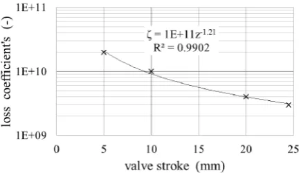
Dependence of cavitation index on the flow rate is shown in figure 3.The graph shows that cavitation occurs already during flow rate 7.87 m3 h-1 for cone stroke 5 mm and for cone stroke 10 mm during flow rate 12.07 m3 h-1. Loss coefficient is typical for control valves used in European countries, which is derived from the equation

2

2 1 2

1

» ¼ º «

¬ ª

Δ =

Ÿ

Δ

= S p

Q p

S Q

ρ ζ

ρ

ζ (6)

Figure 4.

Loss coefficient dependence on the valve stroke.

5 Numerical modelling of flow through

the valve

The task is modelled in a three dimensional space, using plane symmetry. The geometry of the created region, network and boundary conditions are seen in figure 5. Modelled region is identical with the measuring region (figure 1), inlet and outlet of the area are located in places of pressure sensors.

Figure 5.

Geometry of the modelling region, grid and boundary

conditions.

Tasks for cone strokes 5; 10; 20 and 24.5 mm were modeled. In the article only the task for cone stroke of 5 mm, where the cavitation at relatively low flow rates was occurred, is described in detail.

Two equation cavitation turbulent k- RNG model on the basis of the Reynolds number and recommendations of the literature [9, 12, 13] was selected. The third phase i.e. air was added at the inlet so that the pressure and flow rate agreed with the measured values. Volume fraction of air was specified by value of 2% (i.e. air mass flow rate is 3.958·10-5 kg s-1). The task was calculated as a time dependent due to the dynamics of cavitation area. Time step was 0.0001 s, which ensured the convergence of the task at each time step.

Table 1. The measured values for the cone stroke of 5 mm.

Qwater Qwater p1 p2

m3 s-1 kg s-1 Pa Pa

3.278·10-3 3.271 357537 101793

Three variants of the calculation for the cone stroke of 5 mm are compared in this article.

Variant A - water and vapour (two-phase model with

cavitation)

Variant B - water and air (two-phase model without

cavitation)

Variant C - water, air and vapour (three-phase model

with cavitation)

Table 2. Boundary and cavitation conditions for the cone stroke

of 5 mm.

A B C inlet - mass flow inlet* - mass flow rate kg s-1

water 3.271 3.271 3.271

vapour 0 0 0

air - 3.958·10-5 3.958·10-5 outlet - pressure outlet Pa

101793 101793 101793 cavitation

conditions

Schnerr –

Sauer model -

Schnerr – Sauer model

pvap 2340 Pa - 2340 Pa

nb 1013 - 1013

* It is necessary to insert only half of the flow rate into inlet boundary condition because of the plane symmetry task.

Where pvap is saturation vapour pressure; nb is bubble

number density.

Table 3. Physical properties.

density kg m-3 viscosity Pa s

water 998.2 0.001003

vapour 0.017 1.34·10-5

air ideal-gas 1.789·10-5

Turbulent models and grid quality were tested in earlier tasks [11, 12].

6 Evaluation of flow modelling in control

valve

Dependence of inlet pressure on the mass flow rate for numerical and experimental results for selected variants of cone stroke is evaluated in figure 6. It is evident a good agreement between calculated and measured values.

Figure 6. Dependence of pressure inlet (the modeled and

measured) on the mass flow rate.

pressure (as compared with measurement) is greatest for modelling of variant A (flow of water and vapour). The deviation was dramatically reduced by considering the flow of water and air (variant B). The air content in water is equal to 2%. If the cavitation model is added, i.e. the flow of water, vapour and air - variant C, the smallest deviation between calculated and measured values is observed.

Figure 7.

Dependence of inlet pressure and deviation for each

variations of modelling for the cone stroke of 5 mm.

The pressure along the length of the valve for each modelled variants is shown in figure 8. The outlet is given by pressure boundary condition and is specified from experimental measurement, so the pressures on outlet are the same.

Figure 8. Pressure along the length of modelled variants for

cone stroke of 5 mm.

It is obvious that the value of pressure at inlet depends on the choice of the multiphase model, see figure 8. Cavitation model of multiphase flow of water and vapour gives underestimated values of pressure drop in comparison with experiment. The air in variant A is not considered. By addition of air at the inlet the results are significantly more accurate what is confirmed by variants B and C.

From the literature [13, 14, 15] it is evident that air cavitation refines numerical calculation. The amount of air in the liquid is difficult to measure and it is only determined from the numerical experiments.

The volume fraction of vapour in variant A (water and vapour) is significantly higher than in variant C (water, vapour and air), see figure 9. Volume fraction of air in variant B is higher than in variant C. Evaluation of sum of vapour and air volume fraction is only possible for variant C. Comparison of the size of the cavitation area

with the experiment is not possible because the valve is not transparent.

A C

B C

C

Figure 9. Volume fraction of vapour, air, vapour and air for

individual variations vs. length of modelled area.

Figure 10. Cavitation area of the control valve.

Locations where cavitation occurs at the valve by the cone stroke of 5 mm are shown in figure 10. These locations of the valve are the most stressed and greatest wearing occurs on them.

7 Conclusion

The article deals with the formation of cavitation mathematical model for multiphase flow of water, air and vapour in the control valve for individual cone strokes. For verification and definition of the boundary conditions the characteristics and loss coefficients of were measured. Results of mathematical modelling were then compared with experimental results.

arises at low flow rates for the cone stroke of 5 mm. For this reason the cone stroke of 5 mm was also selected for the evaluation of mathematical modelling.

The methodology of mathematical modelling of flow in control valve for each cone stroke was described. From evaluation of numerical solution and experimental measurements it was indicated, that to achieve consensus in the pressure boundary conditions, it was necessary to consider the addition of air, which moreover affects the size of the cavitation cloud.

Numerically it has been proven that vapour and air cavitation occurs at the edges of the valve. In practical point of view, presence of air cavitation reduces wearing in comparison with clean vapour cavitation.

The presence of air and vapour cavitation was also confirmed in other hydraulic elements [13, 14, 15].

References

1. C. E. Brennen, An introduction to cavitation fundamentals. (2011)

2. L. H. Yang, S. A. Liu, Y. L. Chen, X. H. Zhou, C. X. Wang, Y. M. Yao, J. L. Liu, Applied Mechanics and Materials, 548-549 (2014)

3. J. Noskievi, Kavitace. (1969)

4. S. C. LI, Cavitation of Hydraulic Machinery. (2000) 5. C. E. Brennen, Fundamentals of multiphase flow.

(2005)

6. SN EN 60534-2-3 (1999) 7. SN EN 1267 (2012)

8. J. Parish, Valve Magazine. (2009)

9. Fluent 15 – User’s guide. [Online]. Available to from: <URL: http://sp1.vsb.cz/DOC/Fluent_6.1/ html/ug/ /main_pre.htm>.

10. M. Kozubková, Numerické modelování proudní – FLUENT I. [Online]. Available to from: <URL: http://www.338.vsb.cz/seznam.htm>. (2005)

11. M. S. Plesset, R. B. Chapman, J. of Fluid Mechanics, 47 (02), (1971).

12. J. Dobeš, M. Kozubková, EPJ Web of Conferences

67, p. 02019. EDP Sciences. (2014)

13. J. Jablonská, M. Kozubková, Applied Mechanics and Materials, 752-753. (2015)

14. M. Kozubková, J. Rautová, Proceedings of the 3rd IAHR International Meeting of the Workgroup on Cavitation and Dynamic Problems in Hydraulic Machinery and Systems. (2009)

15. J. Jablonská, M. Kozubková, J. of Computational Multiphase Flows, 7 (2), (2015)

Acknowledgements