TAX REFORM IN TUNISIA: A SIMULATION BASED ANALYSIS USING THE NEW AREA-WIDE MODEL

Licensed under Creative Common Page 1

http://ijecm.co.uk/

ISSN 2348 0386

TAX REFORM IN TUNISIA: A SIMULATION BASED

ANALYSIS USING THE NEW AREA-WIDE MODEL

ABDELLI Soulaima

University el Manar, Tunis, Tunisia [email protected]

BELHADJ Besma

University of Carthage, Tunis, Tunisia [email protected]

Abstract

This paper aims to modeling an emergent economy like Tunisia which is rarely used when

calibrating the New Area-Wide Model. Indeed, some modifications and features are introduced

for the calibration of a small open economy of an emergent market. For instance the presence

of the non-Ricardian agents as a financial fraction that is very important when gauging the

impact of tax reform, the wage heterogeneity in the labor market and the risk premia in the

budget constraint. To perform a tax reform, this paper tests the long-run effects of a number of

fiscal consolidation scenarios based on a revenue and expenditure side on the key

macroeconomic aggregates and simulates the economic activity. We discover that the fiscal

consolidation strategy based on the revenue side when lowering distortionary taxes has a

positive long-run effect on the output. Contrariwise, the consolidation strategies based on the

expenditure side has a negative long run impact on the output, but replicates an increase in

the household’s wages as well as the consumption and the investment. The model is calibrated on the Tunisian economy using an annual data over 1980–2011.

Keywords: Tax reform, fiscal policy, DSGE modeling, fiscal consolidation, Tunisia,

Licensed under Creative Common Page 2 INTRODUCTION

Licensed under Creative Common Page 3 in terms of the national tax structures given its significant factor in explaining the differences in the labor utilitisation and the economic performance. In fact the tax wedges in Tunisia is higher than in Euro Area. As the overall tax wedge in Tunisia amounts to roughly 74.3 % of the earnings of an average production worker, while that in the Euro Area is about 64%. Thus Tunisia has an overall tax wedge about 10% points higher than that of Euro Area.

Licensed under Creative Common Page 4 monetary and government spending shock will drive down the output in the medium and the long run while the transfer shock will push up the output in the medium run. For the fiscal revenue side, the strategy based on lowering distortionary taxes, leads to an expansion of the output in the long run .However, the result differs in terms of consumption as it decelerates in the long run when reducing the consumption taxes and rises when reducing labor taxes. Likewise Papageorgiou (2012), it is discovered that the policy instrument followed by the reduction in the consumption tax rate causes a fall in the output which will recover in the long run. Furthermore, the existence of heterogeneous household makes important the distributional effects of the fiscal consolidation (Coenen et al. 2008).The paper is outlined as follows, sections 2 illustrates the specification of the NAWM model focusing on the extension proposed, section 3 provides details about the calibration strategy and performs a dynamic simulation .Section 4 experiments different fiscal consolidation strategies and analyses the dynamic responses of the model as well as the distributional effects under many shocks. Finally, section 5 concludes.

THE MODEL

The model following the spirit of (Coenen et al,2008),consists of two economies of a different population size s and s-1. The novelty in this context is to introduce the Tunisian economy, which is an emergent country, proposed as a home economy and consider the Euro Area as a foreign economy. The foreign economy is modeled exactly in the same spirit as the CMS model. There is an international linkage from the trade of goods and international assets financial markets, enabling imperfect exchange-rate pass-through to consumer prices and financial intermediation costs leading to the imperfect risk sharing. In every country of the NAWM model, there are four types of the economic agents: the households, the firms, the fiscal and the monetary authority. It is assumed that the domestic economy is represented by a continuum of households grouped into two sets I and J. The members of household I are indexed by i



0,1



while the others are indexed byj



1,1



. The first type of household J are called the constrained household or the non ricardian agents .They holds only their labor income, cannot trade in the financial and physical assets ,and have no access to the capital markets and investment choices. The latter differ in terms of their labor skills. Nevertheless, the household I are called ―non constrained‖ or ―ricardian households. They maximize their lifetime intertemporal utility by choosing the consumption good Ci,t _{and the labor services} Ni,t

so they rent services to firms. They also choose the private investment good Ii,t_{to purchase,}

which is linked to the next period physical private capital stockKi,t1

Licensed under Creative Common Page 5 utilization uit_{in production}

. They accumulate physical capital; have access to financial markets, where they trade domestic government bonds of the next period Bi,t1_{and internationally or}

private foreign bondsB

F t

i,1_{. They also hold money for} Mi,t_{for transaction purposes, are with}

better labor skills and have full access to savings technologies. Thus the utility function is defined as follows:









       _         

0       

1 , 1 1 , 1 , 1 1 1 1

k it k it k it k

k

t C kC N

E  

 



(1) 1)

In this case denotes the intertemporal discount factor, σ is the inverse of the intertemporal elasticity of consumption substitution,  is the inverse of the labor effort‘s elasticity relative to the real wage or the Frisch elasticity of labor supply, κ is the external habit persistence or the habit formation in consumption. This function is subject to the period by period budget constraint : M B S B T TR D K P K P u u R N W M B S R rp B B R I P C P v t i F t i t t i t i t i t i D t t i t I K t t i t I it u t i k t k t t i t i t N t t i t i t i F t i t t F F t t i t t i t I t i t c t i v c

t BF W h

1 , , , , , , , , , , , , , , , , 1 , 1 , 1 , 1 , , , , , ) 1 ( ) ) ( ( ) 1 ( ) 1 ( ) ) ( 1 (( )) 1 (                                         (2)

The steady state spread rpbetween the interest rates of foreign and domestic bonds is considered essential in the emergent countries such as Brazil or Tunisia. In fact this risk premia,is included in the budget constraint of the household I ,as As the spirit of De Carvalho and Valli (2011), in order to take in consideration the fact that the real interest rates in Tunisia are substantially higher than in the developed world even in the steady state. Then, St is considered as the nominal exchange rate expressed in terms of units of the home currency per unit of foreign currency. Rt and RF,t_{are respectively the riskless free returns or the interest}

rate on the domestic government bonds and the foreign bonds. BF(BtF) _{is the} financial

intermediation premium that the household member I should pay on their international debt when the external debt deviates from the steady state in the international market. i,t _{is the}

incurred foreign risk intermediation premium rebated in a lump-sum manner in the negotiation of the international bonds. When γBF >0, the domestic household members do not hold internationaly traded bonds and the net foreign asset position is zero worldwide in the stochastic steady state. v(vi,t)_{is the technology transaction cost on the purchase of the consumption good}

Licensed under Creative Common Page 6 households. The household member I hold the stock of contingent securities i,t _{.This latter acts}

as an insurance against the risks on the labor income or the wage income traded amongst all members of these households. Concerning the earning side, Wi,t_{is the wage earned by}

household i for the unit of the labor servicesNi,t_. Pc,t _and PI,t _{are respectively the price of a unit}

private final consumption and the investment good. Rk,t_{is the rate of return on the private}

capital services rented to firms. TRi,tis the transfer‘s payment from the government.Di,t_{is the}

dividend paid by the household-member-owned firms. To finance its expenditure, the fiscal authority takes part of the gross income of the household. It imposes the taxes on different sources of the income like the wage incomeWi,tNi,t_{, the capital income}RKt Ki,t_{, the consumption}

purchases and the dividend Di,t_{income. Where}ct_{is the tax imposed on the consumption}

purchase, Nt is the labor income taxes,tD is the taxes on dividend, W ht is the household‘s

contribution to social security imposed on the wage income, W ht is the tax rate representing the

firm‘s contribution to social security, K

t is the capital income taxes, Ti,t_{is a lump sum only paid}

for the foreign economy. This instrument is chosen to stabilize the debt-to-GDP ratio(De Carvalho and Valli,2011). It depends on the fiscal authority‘s target for the ratio of government debt to output. The capital accumulation owned by the household I depends on the generalized adjustment cost of investment(Ii,t/Ii,t1)_{. The latter is formulated in terms of changes in the}

investment which hinge on the parameter of investment adjustment cost function Iand the

depreciation rate. For its part, the capital utilization cost u(ui,t)_{relies on varying the intensity}

of utilizing the physical capital stock from the steady state ui,tand the capital utilization cost function parametersu,1_, u,2_{>0 . Also it is assumed that both types of the households act as}

wage setters in monopolistic competitive labor markets. As a consequence, they supply sufficient differentiated labor services to firms to satisfy the labor demand. The wages setting

Wi,t_{are characterized by sticky nominal wages set à la Calvo (1983). The household can}

optimally reset their nominal wage contract with probability 1of optimizing each period t. The latter choose the same wage rateWIt Wit

~ ~

,

,  _{as well as the indexation resulting in two separate}

wages Phillips curves. WIt

~

, _{is the optimal wage contract chosen by the household I receiving the}

permission to reset their wage in period t. These households are supposed to maximize the lifetime utility, as defined by equation (1).The other households who cannot optimize, readjust their wagesWi,t_{based on a geometric average of past changes in the price of the private}

Licensed under Creative Common Page 7 inflation. The aggregate wage is based on the two previous equation of the wage setting so that he wage index WI,t_{evolves according to:}

) ) ) (( ) ~ )( 1

(( 1 _{, 1}1 11

2 , 1 , 1 , ,      _{ }

 I I IW I I

P P W

W C It

t C t C I t I I t I        _   (3)

The same reasoning holds for the household J. Turning to the firms, there are two types of firms in the productive sector of the economy indexed by f 

 

0,1.They operate under monopolistic competition with Calvo-type price rigidities. The first one produces the intermediate tradable goodsYf,t _{sold in the domestic market. The second set, produces the non tradable}

final goods like the private consumptionQCt , the private investment Q I

t and the public

consumption goodQGt .The Final goods firms are assumed to operate under imperfect

competition. They combine the imported with the domestic intermediate goods in their purchases. The intermediate good firm‘s f produces its intermediate good outputYf,t _{in the}

competitive markets, with the increasing- returns-to-scale Cobb-Douglas technology, using the homogenous capital services, Kf,t_{, rented from the household I as input as well as the index} of labor services Nf,t_{yielding a technology constraint :}

] 0 , max[ 1 , ,

,  zK N 

Yft t ft ft (4)

Where is the share of fixed cost in production.zt_{is the steady state level of productivity or the}

total factor productivity assumed to be identical across firms. It evolves over time according to serially correlated process. In this casez _{is the autoregressive coefficient of productivity and}z,t

is a white noise shock to productivity. Since all the firms f face the same input prices and have access to the same production technology , the nominal marginal cost MCf,t _{is identical across}

firms that is MCf,t_{= MCt}

. To adapt this model to the emergent country, we follow the approach of Fabia and De Carvalho (2010) and assume that the firms rent labor with unequal labor skills and that the individual with lower level of labor skills are more constrained on their investment possibilities and has lower level of education. This strategy of modeling enable a steady state where skillful workers earn more yet while working the same hours as the less skilled one. In Tunisia the labor contracts require 8 hour work day. The labor input used by firms f to produce the labor output Nf,t _{is given by:}

) ) ( ) ( ) ( ) 1 (( 1 1 1 , 1 1 1 , 1 ,    _         

 N N

N Jft

I t f t

Licensed under Creative Common Page 8 Where  is the population size adjustment to the firm‘s labor demand and the parameter



[0,1/ _{] is added to introduce a bias in favor of a more skilled worker. When} 1 _{this means} that there are equally skilled workers. The parameter > 1 denotes a price elasticity to demand for a specific labor bundles between two households. N

I t

f, _and N

J t

f, _{are expressed in terms of the}

intratemporal elasticity of substitution between the differentiated labor servicesI

, andJof the household I and J. Firms choose the quantity required to hire in both groups of households by taking average wagesWI,t _and WJ,t_{and minimizing total labor cost} N

I t

f, WI,t₊N

J t

f, WJ,t _{subject to}

NJf,t

.It yields from the first order conditionthe aggregate wage index given by:

(6)

In this case WI,t _and WJ,t _{are the nominal wage indexes for the household I and J. While the}

aggregate demand functions for the labor of each group of households J and I are expressed as follow:

N W W

NJft ft

t t J

,

, , 

    

  (7)

As for the households, when taking into account the price setting, each intermediate firms charges different prices at home and sell its differentiated output Yf,t_{in both domestic and}

foreign market under monopolistic competition with calvo price rigidities. Firm f receive permission to set optimally prices PH,f,t _and PX,f,t _{in a given period t with a probability of not}

optimizingH _orX

.

However, the firms which are not allowed to optimize theirprice, adjust their price in the domestic and foreign market such that the price contractsPH,f,t _andPX,f,t _{are indexed to a}

geometric average of the past intermediate good inflation. Where PH,t_andPX,t _{are the price}

indexes and H _and X_{are the indexation parameter determining the weight on the past}

inflation .More preciselyH_{is the degree of domestic price of home good indexation and} X_is

the degree of foreign price of home good indexation (export good).H andX are the domestic

and foreign intermediate goods‘ steady state inflation rates. N

W W

N ft

t t I I

t

f, (1 )( , ) ,



 



 (8)

) ) ( ) )( 1

((  _, 1 _, 1 11

 W W

Licensed under Creative Common Page 9 After aggregating over firms the aggregate price index PH,t_{set by the intermediate good firms f}

for the domestically sold product evolves according to: ) ) ) (( ) ~ )( 1 (( 1 1 1 1 , 1 2 , 1 , 1 , ,                _   P P P P

P H Ht

t H t H H t H H t

H H H (9)

The same equation holds for the aggregate index of the price contractsPX,t _{set for the}

differentiated sold abroad product. As it is mentioned previously for the three types of final good firms, to produce the non-tradable final private consumption goodQCt ,the firms purchases the

domestic and foreign imported intermediate goods respectivelyHCt _and IMCt _{using a}

constant-returns-to-scale CES technology:

) ) 1 ( ) 1 ( ) 1 ( (( 1 1 1 1 1 1 1                           C C C IM C C C C

C C IM

Q IM H

Q _C Ct

t c t C t C t (10)

Where IMC (IM Q ) C t C

t _{is the import adjustment cost faced by the consumption-good firms when}

adjusting the use of imports i.e. its imported share of inputs in the production of the final consumption good. This cost is linked to the import adjustment cost of the consumption parameterIMC _. c1 _{is the intratemporal elasticity of substitution between the bundles of}

domestic and foreign intermediate goods. c_{defines the home bias in the production of the final}

good‗s consumption toward domestic intermediate goods. The weight of the inputs in the consumption basket are defined as (1C) and C.It is worth stating thatH

C

t

f, _andIMCf*t_are

respectively the use of the intermediate goods produced by the domestic and the foreign firm or foreign exporter f and f*. *1 are the intratemporal elasticities of substitution between the domestic and foreign intermediate goods. After choosing the optimal use of each intermediate good f and f* by the consumption good firms, the latter will combine the domestic and foreign intermediate good bundlesHCt _andIMCt _{that minimize the total input cost}P H P IM

C t t IM C t t

H,  ,

subject to aggregation constraint QCt mentioned above so that the unit price of the private

consumption PC,t_{and the demand functions for the intermediate good} HCt _and IMCt _{are obtained}

respectively. The same reasoning holds for the modeling of the non tradable final private investment goodQtI_{.The firms combines its purchase of the domestically-produced intermediate}

goods and the imported foreign intermediate goods respectivelyHtIandIMIt, using a

constant-returns-to-scale CES technology .Then, the final non tradable public consumption good QGt _is

Licensed under Creative Common Page 10 for the domestic intermediate good f HGf,t_{is linked on the unit price of the public consumption}

goodPG,tPH,t

.The demand for the domestic and foreign intermediate goods f and f* areobtained through aggregating across the three final-good firms where:Ht H

C

t ₊HIt₊HGt _and IMt₌IMCt ₊

IMIt. When it comes to the fiscal authority, the CMS assumption is considered. In this case, the

fiscal domestic and foreign authority purchases units of the public consumption goodGtwith

pricePG,t_{,distribute transfer} TRt _{to each household group in unequal amounts, issue bonds to}

refinance its debtBt

, earns seignorage on outstanding money holdings, Mt1, levies taxes on consumption, labor, capital and dividends and adjusts expenditures and budget financing accordingly(See the period-by-period budget constraint of the fiscal authority above).On the expenditure side, two alternative instruments are considered: the real transfer, the real government consumption and the lump sum taxes. Beginning with the government consumption consolidation strategy, the fiscal authority adjusts the consumption spending as a share of steady-state nominal output,gtPG,tGt/PYY_{.This final public consumption good, follows the}

autoregressive process. Thus ρg is the autoregressive coefficient of government consumption and ɛg,t is a white noise shock to government expenditure. Turning to the transfer, the fiscal policy adjust the transfer as a fraction of the steady-state nominal output trtTRt PYY .It is

assumed like Coenen et al.(2007) that the fiscal policy via transfers is unevenly distributed across the two types of household, favoring the households J over the household I. Like (Coenen et al. 2008),it is assumed that the loss in revenue is financed by a decrease in the fiscal authority‘s transfer payments to households such that the government spending and debt-to-output ratios remain unchanged in the long run. The transfer evolves according to the autoregressive process. This is explained by the autoregressive coefficient of the public transfers tr _{.In fact the steady state value of government transfers is defined by} tr _{and the}

white noise shock to government transfers bytr. These expenditures are financed by a diff_erent

types of distortionary taxes, including taxes on consumption spending, labor and capital income. The other distortionary taxes are exogenously set by the fiscal authority considered as constant

 X X

t  _with XC,D,K,N,Wh and Wf. To model the Tunisian monetary authority, we refer to the

outcome of Ben Chalbia (2010) who displayed that the Central Bank of Tunisia is directed more towards the future, precisely a typical Taylor interest rate rule under the forward-looking version featuring the interest-rate smoothing .

 

  



  y s t t Rt

t t

t C

t C R

t R

t g S S

Y Y P

P R

R

R _{g y} 1 ,

1 4

, , 4

4 1

4 ₍₁ _)[  ₍  ₎ ₍  ₎ ₍  ₎

 



Licensed under Creative Common Page 11 This equation is determined in terms of the consumer price inflation and a quarterly output growth to provide an additional information on the future path of the inflation and the output. Also it is crucial to mention that the Taylor equation is enriched with the exchange rate as the Tunisian monetary authority is assumed to follow a flexible exchange rate regime. Where



is the annual inflation target of the monetary authority,R4₌4_{is the annualized quarterly nominal}

equilibrium interest rate, gy is the rate of the output growth in the steady state(assumed to equal 1).The term R,t_{is the white noise shock to the interest rule or the monetary policy shock. It is}

worth to remember that the foreign economy, follows the CMS representation. Also the same formulation are considered for the market clearing conditions holding in the equilibrium, except some modifications in the labor market. These modifications concern the degree of the wage dispersion indices stated in a recursive formulation which are defined as follows:

s W

W

s I ct C It

t I t I I t I I

WIt I I I 1 , 1 1 , , , , ) ( ) ~ )( 1 ( ,      _            (12) s Y P W Y P W

s J ct C Jt

t Y t J J t J J

WJt J J I t Y t J 1 , 1 1 , 1 , , ) ( ) ~ )( 1 ( , ,                              (13)

Where WI,t _and WJ,t _{are the wage inflation rates of the household I and J. The aggregate}

demand for the labour services of variety i and j across the intermediate-good firms are respectivelyNtI _andNJt_{. The same process is considered for the differentiated labor services}

supplied by household J.

CALIBRATION AND SIMULATIONS

Calibration

There are different methods to estimate and evaluate DSGE models. In this case, the model is not estimated but instead calibrated on the Tunisian economy using an annual data over 1980– 2011. Table 1 and 2 summarize the main differences between the block of the two regions.

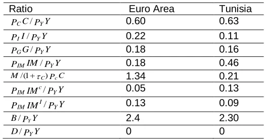
Table 1: Macroeconomic Aggregates (steady state ratios)

Ratio Euro Area Tunisia

Y P C

PC / Y 0.60 0.63

Y P I

PI / Y 0.22 0.11

Y P G

PG / Y 0.18 0.16

Y P IM

PIM / Y 0.18 0.46

C P

M/(1C) c 1.34 0.21

Y P IM

PIM c/ Y 0.05 0.13

Y P IM

PIM I/ Y 0.13 0.09

Y P

B/ Y 2.4 2.30

Y P

Licensed under Creative Common Page 12 The table shows the steady state ratios of the main expenditure categories over nominal output. In order to obtain an accurate result, we try to fit the NAWM to the stylized facts of the Tunisian economy data which is not an easy task for a model adapted to the Euro area. The calibration for the Euro Area is similar to the one of (Coenen et al, 2008). However for Tunisia, we follow the traditional literature and the microeconomic evidence. In fact the national accounts are considered from 1980 to 2011to set the steady-state ratios in the home country. The latter is provided by the International Financial Statistics (IFS) and the World Bank data. However concerning Tunisia ,the parameter‘s value are taken similar to the one of emerging market in the absence of reasonable proxies in the literature. This model involves 138 parameters comprised of aggregate share or ratios, steady state values, 231 endogenous variables and 21 shocks. The table 1 corresponds to the macroeconomic aggregates or the steady state ratios (see the annex1 for more details). The shares of the aggregate demand components in GDP

Y P G P Y P I P Y P C

PC / Y , I / Y , G / Y ) are based on the sample average calculated from the national accounts.

Beginning with the ratio of the private consumption to output _PCC/_PYY_{, it is set to 0.63 in Tunisia.} This value is not far from the one in Turkey which is calibrated to 0.7 by Çebi (2012). To obtain a consistent specification of the steady state trade linkage, it is elementary to calibrate the import to output ratio PIMIM/PYYor the degree of openness, which is 0.4633; the share of import in private consumption goodPIMIMc/PYY that is 0.13 and the share of private investment good

Y P IM

PIM I/ Y which is 0.09 in Tunisia. The money to consumption ratioM/(1C)PcC is 0.21.

Moreover, to measure a country‗s ability to make future payments on its debt, it is crucial to deal with the steady state of the government debt to GDP ratioB/PYY_{. The steady sate ratios of}

government debt to output ratio is fixed to 2.3. For its part, the share of government consumption to outputPGG/PYY, is calibrated to its real value 0.16, on the basis of the annually

IFS Tunisian data.

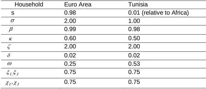
Table 2: Calibrated Parameters and Steady State Variables (Household) Household Euro Area Tunisia

s 0.98 0.01 (relative to Africa)

 2.00 1.00

 0.99 0.98

 0.60 0.50

 2.00 2.00

 0.02 0.02

 0.25 0.53



I, J 0.75 0.75



Licensed under Creative Common Page 13 The dividend income-to-output ratio D/PYY is assumed to be zero in the steady state. Then, the share of private investment to outputPII/PYY is set to 0.11. The calibrated parameters and the

steady state variables concerning the household‘s behavior is exhibited in the table 2 (see the annex 1 for more details). In fact, the financial market frictions w related to the size of the household J is close to 53 %. The rate of time preference or the subjective discount rate is equal to 0.98.The annual depreciation rate of the private and public capital δ amounts to 0.025 across all regions. This value is detected by Ben Aissa and Rebei (2012) and Jouini and Rebei (2014) in Tunisia. It is standard in the literature (see Cooley and Prescott, 1995) or (Burda and Weder, 2002). The production share of capital income in GDP, α=0.3 is opted for Tunisia which is very close to a typical assumption found in the literature usually around 1/3.Hence the estimate seems very reasonable. However, there is no agreement in choosing the magnitude of the inverse intertemporal elasticity of substitution . Generally the estimates are ranging from 1 to 4 in the literature (Lehmus, 2011). In Tunisia it amounts to 1 as the value chosen by Ben Aissa and Rebei (2012), Gouvea et al. (2008); Valli and De Carvalho (2010) in Brazil . The inverse labor supply Frisch elasticity is picked to 2. The range commonly adopted in the business cycle literature is between 1 and 2 especially in the emerging market as detected by Jacquinot and Straub (2008) as well as Gouvea et al. (2008) in Brazil. Our calibration of the degree of habit formation κ is fixed to 0.5, in line with the research carried out by Ben Aissa and Rebei (2012) in the Tunisian economy following the changes in the level of consumption in developing countries. The calibration of the Calvo parameter determining the persistence of wage settingI,J_{, or the fraction of both household members I and J not setting wages optimally}

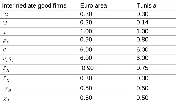
each quarter corresponds to 0.75, consistently with Ben aissa and Rebei (2012) and Jacquinot and Straub (2008). The degree of wage indexationI J is also selected to 0.75. Turning to the

analysis of the table 3 relative to the intermediate good firms. First, the share of the fixed cost in the production  is taken so that to ensure zero profits in the steady state, and discourage the other firms to enter the market in the long run, as documented by Vali and De Carvalho, (2010); Coenen et al. (2007); Christoffel et al. (2008). The value is picked to 0.143, similar to that employed in Emerging Asia (see Jacquinot and Straub, 2008). Second, the steady state productivity level z is normalized to unity (stationary). Third, the calvo probability of the intermediate –good firm‘s fraction selling their differentiated outputs in the domestic markets H

Licensed under Creative Common Page 14 The fraction of foreign firms not setting foreign prices optimallyX _{is fixed to 0.3 and the}

corresponding degree of price indexation X is fixed to 0.5. The intratemporal elasticity of substitution IandJbetween the household-specific bundles for the differentiated labor services,

are designed to 6. This value is also noticed in Brazil by De Carvalho and Valli (2011). On the other side the information related to the final good firms are reported in the table 4(see the annex 1 for more details). The intratemporal price elasticities of substitution between the home and foreign intermediate goods in forming the consumption and investment bundles

 _C, _I

is selected to 1.5.This value is approximate to the one set by Çebi (2012) in Turkey . The home bias parameter, in particular the one that corresponds to the share of domestically-produced goods in the total private consumption expenditure νc, is selected such that it equals its empirical counterpart, precisely as 0.49 in Tunisia. This value is not very far from the one opted in Chile 0.65 by Medina and Soto (2007).

Table 3: Intermediate good firms Intermediate good firms Euro area Tunisia

 0.30 0.30

 0.20 0.14

z 1.00 1.00

z 0.90 0.80

 _{6.00 6.00}



I J 6.00 6.00

H 0.90 0.75

X 0.30 0.30

H 0.50 0.50

X 0.50 0.50

Note: The subscript I represent the unconstrained households while J represent the liquidity constrained household in the model. The same thing for H which stands for the tradable sector while X represents the export sector in the model

Licensed under Creative Common Page 15 percent, expressed as shares of nominal GDP .Moreover, to ensure that the households‘ groups I and J work the same amount of hours, the labor demand bias νw is calibrated to 0.05. Finally, the intratemporal elasticity of substitution designed as the price elasticity of demand between the domestic and foreign intermediate goods for a specific intermediate-good variety is picked to 6, implying a steady-state mark-up of 20%. A common value used in the literature, is confirmed by De Carvalho and Valli (2011) and Galí et al. (2005) for a small open economy in all. The calibration is still pursued with the monetary authority policy that is observed in the table 5. For the parameter related to the interest-rate response coefficients on the annual inflation in term of deviation from an inflation target, also called the interest rate sensitivity to inflation gap

_{,our reference is Çebi (2012) ,who took a mean of 1.5 in Turkey, and Jouini and Rebei} (2014) in Tunisia. Also, based on the calibration of this latter and on Gouvea et al. (2008), the interest rate sensitivity to the output growth gap g y _{corresponds to 0.25 in Tunisia. The}

coefficient on the lagged interest rate or the degree of the interest rate inertia R

, is designated to 0.5 with reference to the prior mean for the interest rate smoothing parameter chosen by Jouini and Rebei (2014) and Çebi et al.(2012). On the other side, the response of monetary authority to exchange rate variation



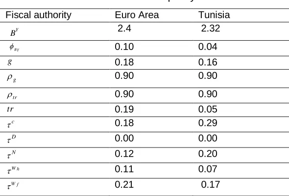
s is set to 0.8.The steady state of inflation π is selected to

1. In the emergent economies like Brazil, this value amounts to 1.04 (seeValli and De Carvalho (2010)). After calibrating the monetary authority policy‘s parametres we now perform the fiscal authority‘s parameters observed in the table 6 (see the annex 1).First, the sensitivity of the aggregate lump-sum taxes with respect to the government debt-to-output ratioBY is designated

to 0.046 in Tunisia which is close to the value proposed by De Carvalho and Valli (2011) and Gouvea et al. (2008) in Brazil. Second, the Government debt-to-output ratio BY_{is set to 2.32.}

Third, the government transfers-to-output ratio or the government transfer (tr_{) is picked so that}

Licensed under Creative Common Page 16 subsequently the social contribution of the employees and employers, 0 for the tax rate on dividend τ D ,as the dividend versed by the Tunisian societies are not submitted to tax and 

N

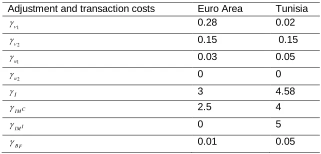
=0.2 for the labor income tax rate. Eventually, table 7 summarize the adjustment and transaction cost. In fact 2 appearing in the functional form of the consumption transaction for

the domestic economy, is opted consistently to Coenen et al. (2008) and Jacquinot and Straub (2008) equal to 0.150.

Table 4: Final good firms

Note: The subscript C represents consumption goods sector while I stands for the investment goods sector. IM means the imported goods sector

For the other parameter 1, we refer to Jacquinot and Straub(2008) in emerging Asia and set it

to 0.029 in Tunisia. In addition, the investment adjustment cost function (the share of domestic good in the investment)I is calibrated to 4.58 in Tunisia based on IFS. In fact, based on the

value of a prior distribution set on Brazil to 4 by Gouvea et al. (2008) or 3 set by Valli and De Carvalho (2010). The capital adjustment cost parameter valueu1is set to 0.05 following Valli and

De Carvalho (2010). In addition to u2 that is picked to 0.007 with reference to Jacquinot and

Straub (2008); Valli and De Carvalho (2010, 2011). For the parameters controlling the adjustment cost related to changing the import share in consumptionIM C, they are detected to 4 in Tunisia based on the value set in Brazil, to dampen the sensitivity of consumption to the change of the terms of trade.

Table 5: Monetary authority Monetary authority Euro Area Tunisia

 1.02 1.00

gy 0.10 0 .25

_R 0.95 0.50

 2.00 1.50

_s - 0.80

Final good firms Euro area Tunisia

C 0.92 0.49

I 0.41 0.50

w 1.00 0.05

C 1.50 1. 50

I 1.50 1.50

Licensed under Creative Common Page 17 This parameter determines the ability of household I to borrow from abroad in the short to medium run. It influences the profile of its intertemporal consumption and investment decision. Besides, the parameters of the import adjustment cost of investment IM I, takes the value of 2.5

(see Jacquinot and Straub, 2008). To end, the parameter governing the intermediation cost function, also called the risk premiumB F_{, is around 0.05 in Tunisia (see Jacquinot and Straub,}

2008) so that the evolution of net foreign assets has a small impact on the exchange rate and the trade in the short run. It enables the net foreign asset position to be stabilized to zero in the long run.

Table 6: Fiscal policy

Note: The calibration of the tax rates of the Euro Area, are similar to the one selected by Christoffel et al.(2008) who provide the information from the OECD (2004) and Eurostat (2006).

Simulation and Policy analysis

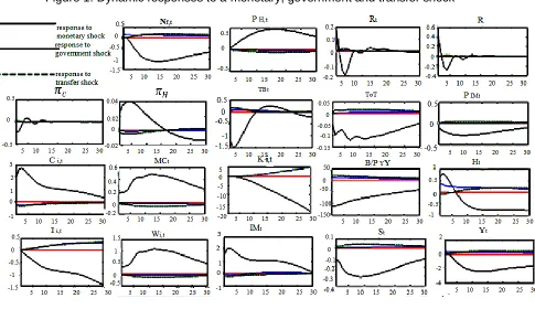
The simulation in this paper concerns the dynamic responses effects of monetary and fiscal shocks like the government spending and the transfer to household shock as well as the dynamic properties of the NAWM illustrated in the figure 1. This figure depicts the dynamic responses of the domestic variables to a monetary policy tightening represented by a black line, equal to a 1% increase in the annualized nominal interest rate; to a persistent government spending shock, represented by a blue line, equal to a 1% increase in the steady- state output and to a persistent transfer shock, represented by a green dashed line, equal to 1% increase in the steady-state output. It is crucial to note that all the dynamic responses are reported as percentage deviations from the steady state. Also, all the simulations were achieved using the function ―stoch_simul‖ of DYNARE at MATLAB.

Fiscal authority Euro Area Tunisia

BY

2.4 2.32

_BY

0.10 0.04

g 0.18 0.16

g 0.90 0.90

_tr 0.90 0.90

tr 0.19 0.05

c

0.18 0.29

D

0.00 0.00

N

0.12 0.20

W h

0.11 0.07

Licensed under Creative Common Page 18 Table 7: Adjustment and transaction cost

Adjustment and transaction costs Euro Area Tunisia

_1 0.28 0.02

_2 0.15 0.15

_u1 0.03 0.05

_u

2 0 0

I 3 4.58

IM C 2.5 4

_{IM I} 0 5

_{B F}

0.01 0.05

The expenditure based consolidation

After the calibration, we describe the dynamic response of the macroeconomic variables following the monetary, government expenditure and the transfer shock.

Monetary shock

After a positive interest rate there is a fall in the output Ytas emphasized by Çebi (2012); Ratto

et al. (2009); Christoffel et al. (2008); Fabia et Valli (2011); Burriel et al. (2010). This decline will put pressure on the consumption and investment and the labor demandNf,t_{. Indeed Christoffel}

et al. (2008) elucidated the drop of the investment by a temporally reduction in the domestic demand. It is crucial to remember the link between the capitalKi,t_{, the interest rate and the debt}

to output ratio. Following this shock, it is noticed that the interest rate declines then moves to zero which will boost the debt to output ratio. De Castro et al. (2011) thought that keeping the interest rate fixed for a certain period yields a fall in the inflation. On the other hand, there is a lower demand for the capital. For its parts, the inflation especially the consumer‘s price inflation

c, slightly pushes up then levels off.

Christoffel et al. (2008) explicated this decline by a fall in the domestic prices. The next variable is the terms of trade ToT_{which is defined by the domestic import price relative to the} export price in domestic currency. Following the monetary shock, it falls then will recover. Indeed, Christoffel et al. (2008) and Coenen et al. (2008) claimed that the improved ToT_{lead to} changes from domestic towards imported goods. More precisely, Coenen et al. (2008) justified this improvement by the appreciation of the domestic currency. When it comes to the real wagesWi,t_{, it is noticed an upward trend in the first 10 quarters that will depreciates in the}

Licensed under Creative Common Page 19 the output. This fall put downward pressure on the domestic priceH.As far as the importIMt is

concerned, there isa continued fall of the latter. In this sense De Castro et al. (2011) pointed out that this fall is caused by the decline in the output. Likewise, the import pricesPIM,t _{dips.Finally,}

we explain the relationship between the trade balance TBt, the real exchange rate and the export. As shown in figure 1, there is a negative impact on the export. That is why the trade balance stabilizes in the long run. Indeed Christoffel el al. (2008) and De Castro et al. (2011) interpreted the reduction in the exports, by the improvement of theToT_{inducing a switching} effect to the imported goods. The real exchange rate, follows nearly the same trends of theToT_.

Figure 1: Dynamic responses to a monetary, government and transfer shock

Transfer shock

As regards the output, the latter hikes in short run, pushing up the consumptionCi,t _{and the}

investmentIi,t_{, then will drop in the long run. Precisely, the consumption decelerates by a small}

Licensed under Creative Common Page 20 in the interest rateRt. For its parts, the interest rate delicately pushes up then levels off

promoting the accumulation of the capital. That is why the debt falls. In addition the wages declines in the medium run then will pushes up for both household. Another pictures emerges with the ToT_{, it rises in the first 10 quarters then will decline in the long run. Finally, we note a} decrease in the trade balance as well as the import.

Government shock

When it comes to the government shock, one can see that the decline of the output is moderate. This is explained by the decrease in the labor supply pushing down the export of the economy. Also the consumption slightly goes down, then will sharply boost in the long run. This is induced by the rise of the employment. At the same time the investment is moving up because of the decline in the interest rate. According to Papageorgiou (2012) and Coenen et al. (2008), the positive impact of the investment is due to the expansion in hours worked that will enhance the marginal product of capital. On the other hand, the interest rateRt goes up just for a short

moment, putting downward pression on the debt. Then will fall in the medium and the long run putting upward pressure on the investment and the consumption. Due to this positive impact on the investment and the increase in hours worked, the capital rises, as discussed by Papageorgiou (2012) and Coenen et al. (2008). Conversely, the inflation has a downward trend, because of the depreciation in the marginal cost of the consumption goods. Concerning the wages, there is an initial decline which will sharply hikes in the long run. Moreover, there is a small decline in the import at the beginning of the period, then will peaks sharply in the medium and the long run. We also note an improvement of the ToT _{(decrease), which is interpreted by} the increase in the imports. In fact, the (TOT) deteriorates the trade balance. This trend can be clarified by the increase in the import in the long run, even if there is a small development in the exchange rate.

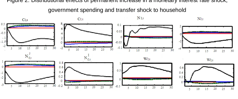
The distributional effect

Licensed under Creative Common Page 21 term as their wage hikes Unlike the consumptionCI,t _{of the household I which is in expansion.}

In this field, Coenen et al. (2008) added that the rise in government consumption absorbs part of the economy's resources yielding a negative wealth impact especially on the part of the household J. As they feel poorer, they will diminish their consumption and improve their labour supplyNJ,t_{. Following the strategy of increasing the transfer, the household J still reduce their}

consumption purchase marginally, then will strongly enhance it. Yet again, Coenen et al. (2008) pointed out that there is a loss of income because of the unequal financing requirement that they face.

Figure 2: Distributional effects of permanent increase in a monetary interest rate shock, government spending and transfer shock to household

The Revenue based consolidation

Concerning the dynamic effect on the revenue- based consolidation, the figure 3 summarizes the impact of a permanent reduction in the consumption and the labor income taxes.

Labor shock

Starting by the labor shock, the latter pushes the output Ytup. In this perspective, Papageorgiou

Licensed under Creative Common Page 22 will boost sharply in the medium and the long run. When it comes to the real wages, Wi,t_the

latter dampens in the short to medium run but rises in the long run. In this context, St𝑎 hler and Thomas (2011) clarified the depression of the wages by the importance of the unemployment. This latter is generated by the drop of the output. On the other hand, the–middle left panel of the Figure 3, shows that the labor income taxes induces an ascension of the capitalKi,t_{. In this}

context Papageorgiou (2012) added that the increases in hours worked has a positive impact on the marginal product of the private capital. The latter encourages the rise of the future capital formation which in return enhances the output in the long run. In the same way Kitao (2010) detected a rise in capital when cutting the temporary income tax. Then, consistently with St𝑎 hler and Thomas (2011), there is a development in the investmentIi,t _{due the fall in the}

interest rate. In fact this fall is detected in the medium and the long run then will levels. The (ToT_{) slightly goes up in the first ten quarters then will decline. Nevertheless, the import initially} cuts down which will then sharply jumps in the long and the medium run. Finally regarding the debt to output, we found that the labor income taxes drives down this debt in the short to medium run. In this perspective, Papageorgiou (2012) précised that the reduction in labor taxes financed by higher consumption taxes not only stimulates the economy but also reduces the debt to output ratio.

Licensed under Creative Common Page 23 Consumption shock

When it comes to the consumption shock, the output sharply declines in the first 10 quarters, then will delicately rises. Besides the consumption initially rises then slightly dampens in the medium and the long run. Furthermore, the real wages initially pushes up then will decline in the medium and the long run .Turning to the (ToT_{), its movement shifts across the time. It declines} then will moderately rises. There is a fall in the capital as well as the investment. Indeed Forni et al. (2009) clarified that the smoother increase in the Ricardian consumption gradually shifts resources away from the investment. So when there is an income increases, the household I does not rely on the economy's capital stock. To end, we should not forget to describe the effect on the trade balance TBt, the import IMt and the exchange rateSt variables. In fact, there is still a reduction in the import yielding an improvement of the trade balance. The latter declines marginally then will picks and stabilize in the long run. Furthermore, the exchange rate goes down. This fall is due to the decline in the export that will in return enhance the debt. Moreover, with the labor income and consumption taxes shocks, the consumer price index cslightly

pushes up in the short run then will stabilize in the medium and the long run. This is also observed by Forni et al.(2009) and St𝑎 hler and Thomas (2011). In fact Çebi (2012) elucidated the initial rise of the inflation by the amelioration of the marginal cost. However, the decline in the inflation puts downward pressure on the interest rate (Forni et al. 2009).

The distributional effect

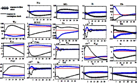
Figure 4: Distributional effect of consumption and labor income tax shock

In an attempt to highlight the influences of the propagation of consumption and labor income shocks on the two types of households ‗s behavior, the figure 4 compares the dynamic responses of many selected variables. It is observed that the consumption tax shock ameliorates the consumption CJ,t _{of the constrained household J when their wage} WJ,t_is

Licensed under Creative Common Page 24 is associated with a slowdown of their labor supply NJ,t_{. To smooth their consumption, they}

should build up their labor supply. However the consumption of the unconstrained household I,

CI,t _{dampen only in the short run, then will recover in the long run. Their wage that witnesses a}

little fall will recognize an ascension. In contradiction, it will depreciates in the medium run. The ensuing drop of the wages followed by a permanent reduction in the consumption taxes explained the depreciation of the non constrained household‘s consumptionCI,t_{. Another cases}

appears with the labor income taxes shock, the distributional effect‗s figure illustrates that this shock encourages the work effort and the labor supply Ni,t _{to hike, as well as the increase in}

hours worked mainly for the constrained household . This is because of the decline in their wages and in their consumption in the short run .The responses of the real wages seems also to follow the one found by Roeger and in‘t veld (2009) especially for the constrained household. However, there is an improvement in the consumption of the non constrained household as their wages rises in the short run, then will drive down.

LONG RUN EFFECTS OF THE TAX REFORM

The table 3 (for more details see the annex1) examines the long-run effects of reducing the level of the tax wedges to levels prevailing on the domestic and foreign variables. In this context, four alternative scenarios are exhibited. The transitional dynamics implied by such reductions is considered. Initiating with the revenue-based-consolidation strategies, the first panel of this table reports the long-run impact of unexpectedly reducing the consumption tax by 11.2%. This instrument affects the decisions of the households along the same consumption – leisure margin and allows them to increase their supply of labor services. In this context Coenen et al. (2008) ensured that the reduction in the consumption tax enhances the labor supply of the economy. However they reported that this technique encourages the purchasing power of the household‘s wage income. While the result displays that the real wage income of the household

Wi,t _{in this case is curtailed by -3.22%.This reduction is also found by Henry el al. (2008) .It is}

observed that the reduction in the consumption tax-rates enables the development of the consumption Ci,t_{by 5.9%. Concerning the capital accumulation}Ki,t_{, it builds up by 83%. In this}

perspective, Coenen et al. (2008) highlighted this behavior by the positive effect of the increase in the hours worked. In return, the investment Ii,t_{is delicately improved by 2.09%.As Burriel et}

al. (2010) and Coenen et al. (2007), we found that an unexpected reduction in the Value Added Taxes (VAT) has a long-run positive effect on the Tunisian economy as the output of the domestic economy Yt hikes by 12.6% .This is explained by the increase in hours worked as

Licensed under Creative Common Page 25 Table 8: Long run effects consolidation in Tunisia and The Euro Area in%

Note: This table presents the steady state effect reported as percentage deviation from the initial steady state for selected domestic and foreign variables of permanent percentage-point reductions in Tunisian tax wedges to levels prevailing in the Euro Area and an increase in the government and a transfer by a 1% of a steady state output

The result shows a slight enhancement of the ToT _{by 0.39%. The other revenue} based-consolidation strategy concerns the reduction in the labor income tax. In a different spirit to Kitao (2010), it is discovered that the labor supply will boost because the wagesWi,t_demanded

by the workers depreciates in this case by -1.524%. In this context, Stähler and Thomas (2011) affirmed that the workers claim weaker gross wages because the reduction in taxation enhances their take-home pay. For its part, the investment Ii,t _{is surging by 0. 96% due to the}

high labor supply as interpreted by Kitao (2010). As a consequence, the economy recognizes a rapid economic growth and a higher output which is developed by 5.799%. As the income becomes higher, our finding displays an expansion in the consumptionCi,t _{which softly peaks by}

2.75%. Although the consumers I increase their consumption more than the household J. For its Revenue consolidation strategy overall

tax wedge

Expenditure

consolidation strategy

Tunisia c0.112 _ _0.068

WN W H0.04 -0.221 g0.0179 tr0.0179

Y 12.60 5.79 4.14 22.59 0.46 -0.09 Ci,t 5.90 2.75 1.97 10.33 -0.23 -0.04

Ii,t 2.09 0.96 0.68 3.75 0.12 -0.01

Y P

B Y 293.47 25.79 18.07 345.24 6.40 4.60

Ki,t 83.97 38.47 27.52 150.30 4.92 -0.63

Ni,t 0.07 0.32 0.23 0.64 0.00 0.00

Nj,t 9.73 1.99 1.40 13.05 0.26 -0.12

Nf,t 5.44 2.49 1.78 9.74 0.16 -0.04

Wi,t -3.22 -1.524 -1.09 -5.51 0.04 0.02

ToT 0.39 0.17 0.12 0.71 -0.00 0.00

IMt 1.07 0.48 0.35 1.92 -0.01 0

HtI 5.76 2.67 1.91 10.17 0.55 -0.04

Euro Area

Y 0.13 0.05 0.04 0.24 0.00 0

Licensed under Creative Common Page 26 parts, the debtBYbecomes higher. Indeed Kitao (2010) revealed that when the labor income tax

rate is kept low, the government budget constraint is satisfied by adjusting the amount of outstanding government debt. This tax cut allows the household to exploit the temporarily high returns from renting additional capital and labor .In this case, the capital goes up by 38, 47%. Besides, the import IMt which slightly hikes by 0,489% .While the exports rises by 2,672%.

Moving to the expenditure consolidation strategy specifically the increase in the transfer. We note a slight negative long run effect on the output by-0.095%. Coenen et al. (2008) explicated that the ascension in transfer dampens the labour supply of the household Ni,t_{for any given}

wage rate especially for the household J while pushes up their disposable income. In the same context, Kitao (2010) justified the shortfall in the labor supply by the income effect as the disposable income rises with higher transfer.

On the other side, the government debt is surging by 4.6% to finance the additional expenditures as explained by Kitao (2010).This rise in the debt crowds out the private capital

Ki,t _{by -0, 63%, and puts downward pressure on the output and consumption. This author}

clarified that the rise in the debt after the transfer policy will put downward pressure on the labor supply and the saving of the households. Turning to the investment, there is a reduction by -0.015% as well as the capital. According to Coenen et al. (2008) this reduction is due to the downturn in the economy‗s capital stock and the reduction in the marginal product of capital. In turn, both the consumptionCi,t_{and the import cuts downs respectively by 0.046%and}

-0.008%.The reduced import will brings down the price of imports PIM,t_{by -0,0073% to restore the}

long-run equilibrium characterized by the balanced trade. As a consequence, the terms of trade ToT_{decelerates by-0.0029 % so that there is an improvement in the}ToT_{. This trend is also} showed by Coenen et al. (2008).

Finally, another scenario will appear if the fiscal authority enhances its government consumption expenditure. This strategy generates a negative wealth effect on the part of households as they cut back consumption purchases by-0.235% (see Coenen et al. 2008). On the other hand, the labor supplyNJ,t _{is developed especially for the household J, by 0.2696%.}

They also emphasized that the investment Ii,t_{boosts (by 0.122 %), due to the positive impact}

of the hours worked on the marginal product of capital. Consequently, this positive impact on the capital and the investment strengthened the output Yt by roughly 0.46%. Also, the exports

Ht is ameliorated by 0.55%. Whereas it pushes down the importsIMt by -0.015%.

Nevertheless, a different behavior appears with the real wages Wi,t_{. It is ameliorated by a small}

Licensed under Creative Common Page 27 MEASURING THE MODEL FIT

For the calibrated model, Malley et al.(2009) suggested two methods to ensure that the model fits the data. For example, the method of Watson (1993) who emphasized on the covariance function ACF and compare the one of the model to the one of the data. Also the method of Christiano et al. (2005) who do the same exercise based on the impulse response function. Both measures need comparison of an estimated VAR with the calibrated VAR. Yet again Lees et al. (2011) reports the match of the model to the key selected moments in the data for the interest rate, inflation, growth rate of output, the change in exchange rate and the terms of trade through the mean, the standard deviation and the distribution of the first order autocorrelation statistics for the estimated model. However we simply compare the theoretical selected moments and implied by the model NAWM to the simulated moments given by the sample data. The table 9 report the mean and variance of the most important endogenous variables implied by the NAWM and the sample moments based on the observed data over the calibration period. Regarding the sample mean as well as the variances, we deduce from Table 9 that the NAWM model broadly fits the data. The variances and the mean of variables obtained from data and that of model are close to each other. The majority of the variables in the table have a data-based (sample) mean that is softly higher than the model-data-based mean. Similarly for the variance, the real GDP, consumption, investment, have a data-based sample volatility measure slightly greater that the NAWM model .

Table 9: Sample mean and variance

Variable mean Variance

simulated theoretical simulated Theoretical

Real GDP 1.832 1.805 0.026 0.019

Consumption 3.14 3.110 0.049 0.038

Investment 0.70 0.599 0.098 0.089

The terms of trade 0.843 0.842 0 0

Nominal interest rate 1.007 1.007 0 0

Real effective exchange rate 0.800 0.797 0 0

Consumption deflator inflation 0.999 0.999 0 0

Debt to output -8.492 -9.065 0 0

Note: For the simulated moments of the variables, the results are based on 2000 draws of the NAWM‘s

structural parameters.

CONCLUSION

Licensed under Creative Common Page 28 propose a reform which demonstrate that both expenditure and revenue-based consolidation measures have an economically significant impact on the macroeconomic aggregates. Depending on the implemented consolidation scheme, it is discovered that the revenue-based consolidation policies when lowering distortionary taxes yields a positive long run effect on the output. In contrast, the expenditure-based policies which deteriorate the output in a long run. However it exhibits a moderate increase in the household wages as well as a slight rise in the consumption in a long run . Also this technique pushes up the investment in a short and a long run. Also, depending on the fiscal instrument used when measuring the impact of the tax reforms, the fiscal consolidation may have a pronounced distributional effects with the presence of heterogeneous households. In future researches many fiscal instruments can be analyzed. For example the techniques proposed by Stähler and Thomas (2011) related to the public investment cuts, the public purchases cuts, the reduction in the public sector employment, the fiscal devaluation ,defined by the decrease in the consumption and the social security contribution tax rate, recently employed in Germany in 2007, the gradual reduction in the debt ratio from its current value to the Maastricht reference value proposed by Coenen et al.(2008),,the rebate transfer suggested by Kitao (2010), the primary surplus target presented by De Carvalho and Valli (2011). Moreover, Lehmus (2011) suggested many fiscal reforms in Finland. For the instance replacing progressive (labor) with a flat tax (consumption or labor), shifting tax burden from labor to a consumption tax, choosing a policy mix when rising the consumption tax. Also Papageorgiou (2012) suggested a technique in Greece to decrease the higher labor tax. Concerning the limits of this study we can emphasize on the lack of the welfare examination of the policy rule for the household in the same way to Kitao (2010) and Papageorgiou (2012). Also not resorting to the Bayesian estimation inference methods of the NAWM model, as Christoffel et al. (2008) and many other authors, giving the accuracy of this approach. Finally not mentioning the sensitivity analysis tackled by many authors (see Kitao, 2010; Coenen et al. 2008) to check the robustness of some results and better understand how the economy works. For example, when varying the labor supply elasticity of households, or the elasticity of substitution between the home and foreign goods on the macroeconomic variables.

ACKNOWLEDGMENT