www.nat-hazards-earth-syst-sci.net/14/1731/2014/ doi:10.5194/nhess-14-1731-2014
© Author(s) 2014. CC Attribution 3.0 License.
Evaluating the effectiveness of flood damage mitigation measures by
the application of propensity score matching
P. Hudson1, W. J. W. Botzen1, H. Kreibich2, P. Bubeck3, and J. C. J. H. Aerts1
1Institute for Environmental Studies, VU University Amsterdam, Amsterdam, the Netherlands 2GFZ German Research Centre for Geosciences, Section Hydrology, Potsdam, Germany 3adelphi, Caspar-Theyss-Straße 14a, Berlin, Germany
Correspondence to: P. Hudson ([email protected])
Received: 24 December 2013 – Published in Nat. Hazards Earth Syst. Sci. Discuss.: 22 January 2014 Revised: 15 May 2014 – Accepted: 26 May 2014 – Published: 15 July 2014
Abstract. The employment of damage mitigation measures (DMMs) by individuals is an important component of in-tegrated flood risk management. In order to promote effi-cient damage mitigation measures, accurate estimates of their damage mitigation potential are required. That is, for cor-rectly assessing the damage mitigation measures’ effective-ness from survey data, one needs to control for sources of bias. A biased estimate can occur if risk characteristics dif-fer between individuals who have, or have not, implemented mitigation measures. This study removed this bias by ap-plying an econometric evaluation technique called propen-sity score matching (PSM) to a survey of German house-holds along three major rivers that were flooded in 2002, 2005, and 2006. The application of this method detected sub-stantial overestimates of mitigation measures’ effectiveness if bias is not controlled for, ranging from nearly EUR 1700 to 15 000 per measure. Bias-corrected effectiveness estimates of several mitigation measures show that these measures are still very effective since they prevent between EUR 6700 and 14 000 of flood damage per flood event. This study concludes with four main recommendations regarding how to better ap-ply propensity score matching in future studies, and makes several policy recommendations.
1 Introduction
The potential risk from flooding is increasing across the world (see IPCC, 2012; Milly et al., 2002; Bouwer et al., 2010; Hall et al., 2005; te Linde et al., 2011). Risk, as de-fined in this paper, is the product of exposure (the value of
a flood risk area to play a role in managing risk. The poten-tial of government investment in this area is relatively more known than that of private households. This paper seeks to add to the nascent literature on this topic.
There are several studies that investigate potential flood damage reduction that can be achieved by various DMMs. For example, Holub and Fuchs (2008) investigate the cost-effectiveness of mitigation measures using a cost–benefit analysis approach, where, if benefits are larger than costs, the measure is regarded as an efficient DMM. Holub and Fuchs (2008) estimate the natural hazard risk posed in their sam-ple area. Once the level of risk is known, the samsam-ple area is divided into different risk zones, and the level of expo-sure within a risk band is used to estimate damage. Holub and Fuchs (2008) then proceed to calculate the benefits of the measures by assuming that a DMM prevents all damage up to a certain severity of hazard. Poussin et al. (2012) em-ploy a similar method by modelling the risk-reducing effect of DMMs, such as wet-proofing a house, by assuming that the effectiveness of a measure is a percentage reduction in flood damage simulated by a flood risk model. Other studies, such as De Moel et al. (2014), Dutta et al. (2003), and DE-FRA (2008), also apply similar methodologies. While these methods are useful, they are not able to empirically evaluate DMMs because they assume, on the basis of expert judge-ment, that the DMMs are effective to a predetermined degree. Damage models, however, do not provide empirical proof that the DMMs are able to prevent damages up to the as-sumed degree. Therefore, studies are undertaken that use household survey data, empirically grounding the evaluation in specific cases, such as Kreibich et al. (2005, 2011) and Bubeck et al. (2012). Bubeck et al. (2012) use a repeated-measure design to compare the amount of flood damage suf-fered by the same households during two consecutive flood events along the German part of the Rhine in 1993 and 1995. To avoid possible bias due to differences in flood hazard characteristics, the most important damage-influencing fac-tor – namely, inundation depth (Thieken et al., 2005) – was controlled for. Only those households were included in the comparison that reported identical water levels in the cel-lar and ground floor during both flood events. This compar-ison reveals a central tendency towards lower flood damage in 1995. Moreover, less extreme damage was recorded for the later event. This trend towards lower flood damage in 1995 is attributed to a considerable increase in DMMs imple-mented by households between the 1993 and the 1995 flood event. Those households that increased the level of DMMs showed the largest reduction in flood damage suffered. How-ever, this method still may not produce an accurate estimate of the effectiveness of a DMM for several reasons. The first is that an explicit value for the effectiveness per DMM has not been provided. The second is that other possible differ-ences in hazard characteristics were not controlled for, such as flow velocity or contamination of floodwater. Also possi-ble changes in household characteristics, such as an increase
in the value of household contents for example, between the floods were not taken into account.
A different survey data methodology is that of Kreibich et al. (2005, 2011). In these studies a more direct estimate of effectiveness was provided. In Kreibich et al. (2005), for the various DMMs, households were divided into those who have employed a particular DMM and those who did not. Once the sample has been divided into two groups based on the use of a DMM, the average damage suffered in each group is calculated, and the difference between these aver-ages forms the estimated effectiveness. These results are im-portant initial steps regarding the evaluation of DMMs. How-ever, a drawback of this approach is that the difference in average damage suffered between the treatment (those who installed a DMM) and the control (those who did not install a DMM) groups may still not provide an accurate estimate of the damage savings obtained by the DMM, since other factors could have influenced the difference in damage, such as inundation depth, flow velocity, or differences in house-hold characteristics. Kreibich and Thieken (2009) employ a similar method to examine the success of DMMs in Dres-den. In particular, they estimate the mean difference in dam-age between individuals who suffered roughly similar natural hazard risks, and refine the DMM effectiveness estimate by removing a source of bias, but still leaving several factors un-controlled for, and creating problems due to very small sam-ple sizes (treatment groups of 3–5 households). Finally, the later study of Kreibich et al. (2011) had an additional benefit to its micro-scale cost–benefit analysis due to using a sam-ple consisting of structurally identical households. The iden-tical household construction removes some sources of bias. However, the approaches employed have meant that poten-tial sources of bias have been independently controlled for. These issues result in a direct effectiveness estimate, but one that is potentially inaccurate due to the presence of selection bias.
may be overestimated by a mean comparison methodology. PSM removes selection bias by using the probability of em-ploying the treatment, the propensity score (PS), to match individuals. The researcher finds, for each agent in the treat-ment group, at least one member of the control group with the same or sufficiently close PS to make a match. Having a similar-enough PS guarantees that the selection bias has af-fected the matched respondents in an equally powerful way. Therefore, by comparing the outcomes (e.g. flood damage suffered) of individuals with a similar PS, selection bias is removed and an accurate estimate of the treatment effect is provided.
D’Agostino (1998) notes that PSM has been applied to a wide range of research topics. In medicine it is commonly used to study the effectiveness of drugs or surgical methods. For example Vincent et al. (2002) investigate the effective-ness of blood transfusions when the patient is critically ill and suffering from anemia. In economics, PSM is applied to a wide variety of economic issues. For example, Dehejia and Wahba (2002) provide an evaluation of the effects of taking part in a government-training programme on incomes. In the above cases, PSM is used because the most reliable method of estimating the treatment effect, a controlled randomised trial, is unfeasible due to practical and/or ethical concerns, and therefore a different technique is needed.
The objectives of the current paper are two-fold. The first is to remove selection bias that may be present in previous DMM effectiveness estimates, in order to produce a more accurate estimate of DMM effectiveness. The second is to judge the applicability of PSM to wider natural hazards re-search. To the best of our knowledge, this paper is the first study to use PSM to evaluate the installation of flood DMMs. Furthermore, only one other study has applied PSM to nat-ural hazards: Butry (2009), who investigates the success of wildfire mitigation programmes. The current paper seeks to apply PSM to provide a bias-free estimate of the flood dam-ages prevented due to DMMs, which will be useful in guid-ing integrated flood risk management strategies and the role individuals can play in mitigating flood risk.
The remainder of this paper is structured in the follow-ing manner: Sect. 2 describes the PSM method; Sect. 3 pro-vides a description of the data collection; Sect. 4 presents the estimation results; Sect. 5 discusses the main findings; and Sect. 6 concludes.
2 Method: propensity score matching (PSM)
To evaluate a treatment, in this study of the use of a private DMM, it is required to make an estimate of the difference between what occurred and what would have occurred if the agent had the opposite treatment participation. This is the av-erage treatment effect on the treated (ATT), which is defined in Eq. (1). Below,E(.)is the expectations operator;T is a bi-nary variable for participation in the treatment group or not;
y1is the outcome under treatment; whiley0is the outcome under non-treatment:
ATT=E (y1−y0|T=1)=E (y1|T=1)−E (y0|T=1) . (1) A positive ATT indicates that participation in the treatment is expected to increase the outcome variable, while a nega-tive value indicates a reduction. For a DMM, a highly neg-ative ATT would indicate that it was effective at mitigat-ing flood damage. However, either the outcome under treat-ment (E (y1|T =1)) or the outcome under non-treatment (E (y0|T =0)) is observed. Therefore, for individuali the ATT cannot be constructed, as only the first half of Eq. (1) is known. The intuitive method of recreating the counterfactual observation is to use the respondents who did not take part in the treatment. Angrist and Pische (2009) provide a gen-eral expression for the difference between sample sub-group averages, showing the potential combination of the ATT and selection bias (SB):
E (y1|T =1)−E (y0|T =0)
=E (y1−y0|T =1)+E (y1−y0|T =0)
=ATT+SB. (2)
Selection bias is present (SB6=0) if there are traits that ex-plain both participation in the treatment and outcomes, and where these traits differ across these two groups. These traits are confounders, and their influence on outcomes and partic-ipation masks the true value of the ATT. If there were ran-dom entry into the control and treatment group, treatment participation would no longer be tied to individual traits. This means that the difference in mean damage between the two groups would provide an unbiased estimate of the ATT, which is the rationale behind a controlled randomised trial. However, while randomised trials will provide an unbiased estimate of the effect, Grossman and Mackenzie (2005) ar-gue that a controlled randomised trial can only provide a re-liable estimate if behaviour can be monitored and outcomes observed during the trial period. A trial for DMMs is in prac-tice unfeasible due to the organisational requirements, costs, and unpredictable nature of flood events. There are also eth-ical concerns about forcing the control group to remain un-prepared for potential disasters. Therefore, survey data and observational outcomes must be used, which, in turn, means that entry into the treatment group is non-random and driven by traits such as total exposure or perceived risk, making se-lection bias a potential problem. In such a case PSM can be used to estimate the ATT.
estimate of the ATT. Originally, matching was based on co-variates, where a researcher would attempt to find individu-als who have the same values of the confounding covariates, and match these individuals. However, this can be problem-atic or even impossible with large numbers of confounders. Identical individuals are easy to find if there are only two bi-nary confounders, and thus only four possible combinations to group respondents. But this becomes more difficult, the more relevant confounders there are that must be included in the matching process, and even more complicated if these variables are continuous rather than binary variables. For ex-ample, if matching takes place based on whether the build-ing is located in an urban area, then urban treatment group members can be matched with urban control group members. If household content values are additionally matched upon, then control and treatment group members who are both ur-ban and have an equal contents value must be found. Then if house size is also matched, matches must be identical in all three respects. This dimensionality issue can greatly reduce the possible sample size. Matching on the PS removes this dimensionality issue as the estimated PS compresses the rel-evant information into a single value. PSM allows a match to be made by finding two, or more, agents with a sufficiently close PS.
For PSM to be valid the following three conditions are re-quired to hold, where ⊥represents independence; X is the set of observable traits; p(X)is the propensity score as a function of the observable traits;T is a binary variable for participation in the treatment group or not; andy1is the out-come under treatment, while y0 is the outcome under non-treatment:
Condition 1: Unconfoundedness –(y1, y0)⊥T|p(X); Condition 2: Balancing –T⊥X|p(X);
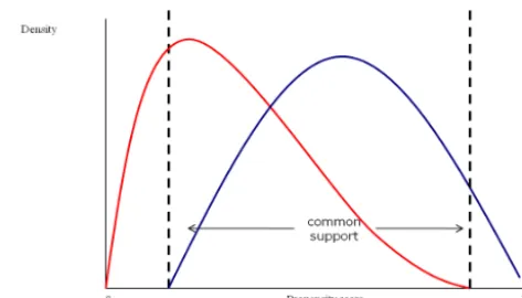
Condition 3: Overlap – the probability distributions for the control and treatment group share a common sup-port, as in Fig. 1.
Condition 1 means that treatment participation and poten-tial outcomes are independent of one another, conditional on the PS; in effect achievingy1ory0is as good as random. The role of Condition 1 is that, by conditioning on the set of con-founders, the selection bias in the treatment is removed. Un-confoundedness holds when all the confounders have been included in generating the PS.
Condition 2 is that, when conditioned onp(X), treatment participation and individual traits are independent of one an-other. When Condition 2 holds, the PS is a balancing score, and then matching on the value of the PS achieves the same as conditioning on each individual confounder value.
Condition 3 implies that the observations have a similar-enough PS to create a good match of individuals. Heckman et al. (1996) provide a formulation of the bias introduced due to matching, showing that the smaller the common support,
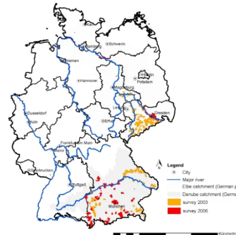
Figure 1. A map of the survey locations and river catchment areas.
the greater the possible bias in the final estimate (an exam-ple of a common support is displayed in Fig. 1). The reason is that outside this range the matched participants are poten-tially too different from one another. Heckman et al. (1996) then proceed to state that by only matching over PS located in the common support this matching quality bias is removed. Matching quality bias is introduced when matched individu-als are too different from each another.
Taken together Conditions 1 and 3 remove bias from the estimate, while Condition 2 allows for matching based on a single value constructed from all the confounders.
In most cases, a probit or logit model will estimate the PS1. It has been found that using an estimate of the PS rather than the true PS (the actual probability for an individual to employ a DMM) can increase efficiency (Rosenbaum, 1987; Robins et al., 1995; Rubin and Thomas, 1996; Heckmen et al., 1998; Hirano et al., 2003). The variables to be included in the PS model need to meet the aims of Conditions 1 and 2. Brookhart et al. (2006) find that including variables that are only connected to outcomes tends to reduce the variance of the final estimate, while variables that only affect participa-tion tend to increase the variance. Taken together, this implies that variables connected to outcomes should be included; their inclusion reduces bias or at least reduces the variance
1These are non-linear regression models; the advantage of these
of the model2. However, there is a trade-off because the more variables in the PS function, the smaller the potential overlap between the probability distributions.
The evaluation of the PS is not focused on the quality of the PS estimates, in the sense that the estimated PS is close to the true PS, or that the regression used to estimate the PS is consistent (unbiased). The role of the PS is solely to col-lapse the relevant information into a single value, which is achieved upon balancing (Rosenbaum, 2002). Furthermore, the actual estimated coefficients of the probit or logit model are also unimportant; evaluation is based solely on achiev-ing the conditions of balancachiev-ing, unconfoundedness, and suf-ficient overlap.
Once Conditions 1–3 are deemed to hold, a matching al-gorithm must be selected. The alal-gorithm will find for each agent in the treatment group (a) member(s) of the control group who has (have) a similar-enough PS, and these two are matched; the average difference between the outcomes (flood damage) of the matches is an estimate of the ATT. There are several methods for the matching process:
1. Nearest-neighbour matching: a match is the person with the closest PS to the observation of interest, but located in the control group. However, it may be that the near-est neighbour is very far away, in terms of the PS, in-creasing the potential bias of the estimate, due to poor-quality matches. With this method, matching with, or without, replacement can have a large effect. This is be-cause by matching without replacement, an individual is out of the sample once it has been matched. If this individual would have been a good match for another agent, then a worse match for that agent must be made. Matching with replacement solves this issue, and the or-dering of data will no longer be important, but the use of less unique information can increase the variance. The trade-off to be made is between bias reduction (match-ing with replacement) and precision (match(match-ing without replacement).
2. Caliper/radius matching: caliper matching creates a match by accepting any PS as viable if it lies within a bandwidth around the PS in which we are interested in for example±2 %. The benefit of this method is that the number of bad matches will be reduced due to the bandwidth. However it is possible that fewer matches may be made compared with nearest-neighbour match-ing, as, if no agent is located inside the caliper, then there is no match. Radius matching is an extension of this approach because it matches all the observations 2If the unconfoundedness assumption holds, each matching
es-timate will tend towards the same value. However, if unconfound-edness does not hold, then adding variables that only influence out-comes will not mean that the different matching estimates will al-ways tend towards one another, as each matching method may be centred around a different expected value.
found inside the bandwidth. There is no strong reason to select one bandwidth over another, a priori, as there is a trade-off between the number of matches that can be made against the bias of the matches.
3. Stratification matching: the area of PS overlap is par-titioned into intervals or strata. Each stratum is defined over a specific range of the PS, e.g. [0.1, 0.3], and within each strata there are no statistically significant differ-ences between the traits of the treatment and those of the control groups. The overall ATT is estimated by first solving for the ATT within each strata, and then using a weighted average of the strata ATT. These strata are commonly the same as those used to test the balancing assumption.
4. Kernel matching: kernel models use a weighted average of all of the observations in the control group to create matches for the members of the treatment group, where the greater the distance between the PSs, the lower the weight. As such models use all the members of the con-trol group to create a counterfactual observation for a treatment group member, bad matches will be included in the process. However, the weighting process reduces the influence of bad matches, mitigating their influence. The bandwidth of the kernel is very important, as it de-termines the degree of smoothing, and large bandwidths may introduce bias into the estimated ATT. While the bandwidth is important, it is unclear what the correct bandwidth is before the investigation begins. Selection of the bandwidth should be treated as a trade-off be-tween bias and variance.
The following PS function will be estimated, whereϕ(.)is the standard normal distribution CDF,θis a vector of coeffi-cients,xit is a vector of explanatory variables, andεit is the error term
Tit=ϕ θ0+θ0xit+εit
, (3)
wherexitconsists of confounding variables that explain both participation and outcomes, or at the least outcomes. Vari-ables that only explain participation are to be avoided. Once this model has been estimated for a given vector ofxit, the balancing assumption will be tested, as a series of T orF tests within each supposed PS strata. In effect, the sample is stratified by PS and tested for a lack of systematic differ-ences between the control and treatment group members of that stratum. When balance is achieved, the matching pro-cess will be carried out. If balancing is not achieved, addi-tional variables will be added to thexit vector until balance is achieved. The fitted value of Eq. (3) is the PS that is used to create matches.
The vector of confounding variables will be guided by economic intuition. The economic incentive to undertake a DMM is the savings due to the installation of the measure over the measure’s lifetime. The damage generated by a flood can be viewed as coming from the following process: Damageit =F Hazardit,Exposureit,Vulnerabilityit
. (4) Each element of Eq. (4) is positively related to the damage outcome. The incentive to employ a DMM is based more on expected damage – the individual’s perception of the risk faced – but expected and actual damage may be similar in construction. This economic framework means that there will be a large overlap between the incentive to employ a DMM and the final outcome, and, as such, the major confounders can be found by focusing on the elements of Eq. 4.
3 Data
3.1 Survey description
The data were collected via two surveys, one after the flood in 2002, and another one after the floods in 2005 and 2006 in both the Elbe and the Danube river catchments in Ger-many (Kreibich et al., 2005, 2011; Thieken et al., 2005; Kreibich and Thieken, 2009). On the basis of building spe-cific random samples of private households in flood-affected areas, computer-aided telephone interviews were undertaken in April and May 2003 and in November and December 2006. These surveys resulted in 1697 and 461 completed in-terviews with private households, respectively. These were large-magnitude flood events, as the 2002 flood caused an es-timated total direct damage of EUR 11.6 billion in Germany (Kron, 2004). The flood history of the two catchment areas is quite different. Before 2002, the last major flood that had
37 1
2
Figure 1. An example of a common support
3 4 5 6 7 8 9 10 11 12 13 14 15 16 17 18 19
Figure 2. An example of a common support.
occurred along the Elbe was in the 1950s, while along the Danube a major flood had occurred in 1999 (Thieken et al., 2005). Figure 2 presents a map of the catchment areas, as well as an indication of the areas surveyed to provide infor-mation on household flood preparedness and consequences of the floods.
The questionnaires addressed the following topics: emer-gency and precautionary measures; flood experience; flood parameters (e.g. contamination, water level); socio-economic parameters; and flood damage. The sample provided by the surveys is trimmed in two respects. The first is that any observations with damage over EUR 100 000 are removed when investigating contents damage and over EUR 300 000 when investigating building damage, as these respondents are strong outliers, and there are few of these observations regarding the sample that can be matched. Furthermore, if these individuals are included in the sample, the balanc-ing assumption could not be achieved, and the methodology could not be applied, as described in Sect. 2.
3.2 Variables
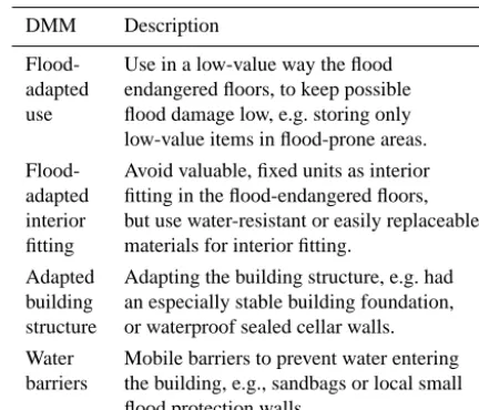
A brief description of the DMMs investigated in this study is provided in Table 1; a more detailed description can be found in Kreibich et al. (2005, 2011).
The confounding variables are described in Appendix A, but the intuition behind their inclusion is explained here. The variables have been divided into categories based on the ele-ments of the Crichton risk triangle and Eq. (4). The category assigned to each variable is not important for the PSM model. Rather, the categories are used to determine the variables de-rived from the survey that can influence flood damages. To control for exposure, the value of household contents (for contents damage) or the house price (for building damage) has been included. House prices and contents values fully capture exposure, as they represent the value at risk, where greater values indicate greater potential losses from a flood.
Table 1. Flood DMMs.
DMM Description
Flood- Use in a low-value way the flood adapted endangered floors, to keep possible use flood damage low, e.g. storing only low-value items in flood-prone areas. Flood- Avoid valuable, fixed units as interior adapted fitting in the flood-endangered floors, interior but use water-resistant or easily replaceable fitting materials for interior fitting.
Adapted Adapting the building structure, e.g. had building an especially stable building foundation, structure or waterproof sealed cellar walls. Water Mobile barriers to prevent water entering barriers the building, e.g., sandbags or local small
flood protection walls.
has a cellar as these houses generally experience higher flood damage (Kreibich et al., 2011), the age of the building, the quality of the building materials, and whether the building is located in an urban environment. Floor space is used to proxy the size of the building, as larger buildings may be more likely to come into contact with floodwaters. Where required, either to reduce an ATT’s variance or to achieve the balancing assumption, the quality and duration of a flood warning was also included. A warning provides time to make sure that static DMMs are used correctly or allows mobile measures, like “water barriers” for example, to be employed. The following variables are used to control for the haz-ard that the respondents faced: flood water height inside the building; flood duration; contamination of flood water; the return period of the flood; velocity; flood experience; whether the building could not be used while flooded; and whether the building is located along the Elbe river (as com-pared to the Danube river).
It should be noted that above variables might not be use-able for all potential PS functions that analyse a DMM. This is because a variable should be reasonably unaffected by the use of the particular DMM, and certain measures are aimed at directly altering these variables. This problem occurs with water barriers, which potentially affect water height, flow ve-locity, and the duration that a building was flooded. In prin-ciple the same set of confounders is used to construct the PS for each DMM. However, when certain variables were included it proved impossible to achieve the balancing as-sumption. Therefore, not every variable could be included in each PS function. The list of variables included in each PS function is displayed in Table A1.
In order to retain as much information as possible and to achieve the balancing assumption, the survey variables were coded in the following manner. Where a variable was cate-gorical, the categories were treated as separate binary
vari-ables, and a binary dummy variable was created for each cat-egory. Variables such as water height and duration were left as continuous variables.
However, occasionally one of the categorical confound-ing variables was dropped from the PS function. Removconfound-ing a categorical confounding variable will not completely re-move all of the information contained by this variable3, pos-sibly only altering the variance of the model. However, there is a core set of variables included in each PS function based on housing type and quality; whether the building has a cel-lar; total floor space; building/contents value; building age; experiences relating to the 2002 (or later) flood(s); warning duration; and how often the individual has been affected by flooding in the past. These variables as a whole capture the elements of Eq. (4) quite well. For example, contents value would capture the level of contents exposure completely. The methodological approach followed was that the core ables are included in every PS model, and additional vari-ables are added as required to achieve balance or to improve the variance of the estimates.
Once the PS has been estimated, only observations with PSs within the common support are retained. The com-mon support is determined by removing any observa-tion that has a PS that lies outside the following range: [max PScontrolmin ,PStreatmentmin ,min PScontrolmax ,PStreatmentmax ].
4 Estimation results 4.1 ATT estimates
The ATT estimates are presented in Table 2 for the five matching methods used. Several methods were used to test the consistency of the ATT estimates, and infer the validity of the confounding variable vector. In particular, the ratio of the standard deviation to the mean of a set of ATT estimates was calculated as a consistency indicator (Table 2). This in-dicator ranges in value from 0.04 to 0.54, where the smaller the value, the smaller the spread of ATT estimates. Some of the DMMs have ATT estimates that are very strongly con-centrated around a central value. As an illustration, for the significantly effective DMMs (the effective measures, though water barriers are only partial successful), the above consis-tency indicator ranges from 0.04 to 0.08. However, for the ineffective measures the indicator ranges from 0.12 to 0.54. This indicator is especially large for “adapted building struc-ture”, namely 0.33–0.54, implying that a confounding vari-able may be missing from the PS function due to the greater spread of estimated ATT values.
In order to have an overview of the potential bias in a DMM’s estimated effectiveness a mean comparison is 3When a categorical variable is converted into a series of dummy
Table 2. Estimates of the effectiveness of private DMM [in Euros].
Flood-adapted Flood-adapted Water Adapted building use interior fitting barrier structure
(contents
damage)
(b
uilding
damage)
(contents
damage)
(b
uilding
damage)
(contents
damage)
(b
uilding
damage)
(contents
damage)
(b
uilding
damage)
Nearest-neighbour −6386c −13 943b −5255a −10 276a 4099 −8543 −2608 −1032 matching (2364) (6694) (3099) (6030) (4162) (6675) (3470) (9036) Radius matching −6923c −13 574c −4536c −10 660c 4837 −8404a −1521 −2281 (2059) (4853) (1919) (4237) (2964) (4465) (2629) (6236) Stratification matching −6649c −16 042c −5217c −11 478c 4034 −8263a −1211 −3856 (1660) (5519) (1889) (3354) (2760) (4987) (3078) (5828) Kernel matching −7092c −16035c −5830c −12 630c 3408 −9438b −1885 −5235 (Gaussian) (1599) (4469) (1814) (3347) (2749) (4402) (2653) (5577) Kernel matching −6608c −14 793c −5170c −11 466c 4110 −8108a −1339 −2478 (Epanechnikov) (1581) (4644) (1598) (3659) (2800) (4373) (2670) (5726) Mean comparison −8415c −21 968c −9063c −25 817c −713 −15 486c −1326 −13 888c
(1361) (374) (459) (3915) (1594) (4315) (1760) (4564)
Matches 85 93 80 88 68 80 55 60
Bias −1683 −7583 −3861 −14 515 −4811 −6935 −387 −10 912 Average ATT estimate −6732 −14 385 −5202 −11 302 4098 −8551 −1713 −2976 Spread of ATT estimates 0.04 0.07 0.09 0.08 0.12 0.06 0.33 0.54 Effective DMM Yes Yes Yes Yes No Yes No No
Notes:a,b,cstand for statistical significance at the 10, 5, and 1 % levels, respectivily. The numbers in brackets are standard errors. Where analytical standard errors are not
available, they have been calculated via bootstrapping with 2000 repetitions. The ATT estimates above have been rounded to the nearest whole Euro. The ATT’s change in expected flood damages due to a DMM is given; i.e. the more negative the ATT, the more effective is the DMM in mitigating flood damage. The spread of ATTs is measured by the ratio of the standard deviation to the mean of ATT estimates.
also carried out similar to that of Kreibich et al. (2005, 2011). However, the results are not directly comparable with Kreibich et al. (2005, 2011), as these previous studies used (slightly) different data, and the dependent variable here is the absolute value of damage suffered rather than the flood damage proportional to exposure. The former is reported here since it improves the interpretability of the results by generating an explicit value for damage prevented.
The estimated ATTs show that once PSM has removed the sources of bias originating from exposure, vulnerability, and hazard, several DMMs are still effective at reducing flood damage (Table 2). Four sets of ATT estimates are highly significantly different from 0 (past the 1 % level): these are the DMMs “flood-adapted use” with respect to contents and building damage, and “flood-adapted interior fitting” with re-spect to contents and building damage. A fifth ATT set is marginally significant at the 10 % level: this is water bar-riers with respect to building damage. This indicates that these DMMs are the most effective ones out of those
al. (2013). It may also be simply an idiosyncratic feature of these flood events, and for a different series of flood events the potential bias may be reversed. Exposure and vulnera-bility indicators seem rather similar across the two groups. While exposure and vulnerability indicators are required to remove bias in the estimated ATT, because they are impor-tant confounders at an individual level, the larger degree of difference in hazard seems to be the major source of bias in this application. The reason is that these distributions are most divergent across the groups. Therefore, a simple mean difference in damage fails to account for the differing sever-ity of the floods affecting the control and treatment group.
The DMMs flood-adapted use and flood-adapted inte-rior fitting are still very effective when bias has been re-moved, as these measures have prevented, respectively, about EUR 6700 and 5200 of contents damage. The selection bias present in mean comparisons is rather substantial, as for flood-adapted use the bias is 25 % of the size of the estimated ATT, while, for flood-adapted interior fitting, the selection bias is 74 % of the size of the ATT. Selection bias appears to be a very powerful masking force in a mean comparison.
It appears that flood-adapted use (e.g. storing only low-value items in flood-prone storeys) is more effective than flood-adapted interior fitting (e.g. using flood-resistant mate-rials to construct interior fittings) for reducing contents dam-age, which is most likely because the former is a direct mea-sure for limiting the impacts of floods on contents, while flood-adapted interior fitting would be an indirect way of reducing contents damage due to storage units being more flood safe. The two measures work by altering different as-pects of Eq. (4); flood-adapted use alters the effective level of exposure, while flood-adapted interior fitting would reduce the vulnerability of household storage units.
The measures that are effective at reducing building dam-age – i.e. flood-adapted use, flood-adapted interior fitting, and water barriers – again suffer from a substantial bias of EUR 7583, 14515, and 6935, respectively. As a percentage of the ATT, this bias is 55, 128, and 81 %. The bias regard-ing buildregard-ing damage as a proportion of the ATT is, on the whole, larger than that present in the estimated ATTs relating to content damage. Flood-adapted use, flood-adapted interior fitting, and water barrier are still potentially very effective DMMs, preventing EUR 14 385, 11 302 or 8551 of building damages, respectively. Flood-adapted interior fitting is more effective than water barriers at reducing building damage be-cause it has reduced the vulnerability level of the building. Water barriers would reduce the amount of water entering the house, but, dependent on the magnitude of the flood, may be overtopped and then would not work at all. Considering the magnitude of the floods suffered, which was up to a 1 in 500-year return period in some cases (Risk Management So-lutions, 2003), it may be that water barriers may be more ef-fective at reducing building damages incurred from smaller-magnitude flood events. The series of strategies represented
by flood-adapted use would have caused its reduction in dam-ages due to lower levels of exposure in floodable areas.
Adapted building structure was, via a mean comparison, detected to have no significant effect of reducing contents damage, and, even controlling for bias via PSM, it is still ineffective. A further finding is that, if nearest-neighbour matching is ignored, then the average bias is only about EUR 150. Such a remarkably close estimate in a small sam-ple could mean that, for this measure, its imsam-plementation could be almost as good as random. If all estimated ATTs are included, then the bias increases to 16 % of the average ATT for this DMM. This observation reinforces the misleading nature of mean comparisons because sometimes a mean com-parison is an accurate estimation technique, while in other cases it is not. The results for adapted building structure regarding building damage are the most inconsistent set of ATT estimates. This may indicate that there is a missing con-founder in the relationship between adapted building struc-ture and building damage, as, if the whole set of confounders was found, then the estimated ATTs should be closer together in value. This inconsistency means that any inference about adapted building structure and building damage (and to a smaller degree contents damage) should be treated with cau-tion.
The measure that seems most effective is flood-adapted use as it has a substantial impact on both building and con-tents damages, being closely followed by food-adapted inte-rior fitting. Flood-adapted inteinte-rior fitting may be less effec-tive because damage in this paper is measured via replace-ment values; flood-adapted use aims at reducing this value while flood-adapted interior fitting does not. An interesting observation from the ATT estimates is that water barriers had a very different effect on contents and building damage. The same measure had a positive (insignificant) ATT regarding contents damage and a negative ATT for building damage, from which it can be inferred that water barriers were ef-fective at protecting the building but not its contents. This could be an artefact of an incomplete set of confounders, but this argument fails to explain why water barriers protect the building. Compared with the other measures that protect household contents the use of water barriers may have re-duced an individual’s efforts to take other measures that limit flood damage.
4.2 Sensitivity analysis
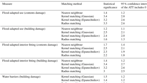
Table 3. Sensitivity analysis.
Measure Matching method Statistical 95 % confidence interval significance of the ATT includes 0 Flood-adapted use (contents damage) Nearest neighbour 1.4 1.2
Kernel matching (Gaussian) 3.4 2.8 Kernel matching (Epanechnikov) 3.2 2.6 Radius matching 3.3 2.6 Flood-adapted use (building damage) Nearest neighbour 1.2 1.1 Kernel matching (Gaussian) 2.5 2.1 Kernel matching (Epanechnikov) 2.4 2.0 Radius matching 1.6 1.3 Flood-adapted interior fitting (contents damage) Nearest neighbour 1.7 1.4 Kernel matching (Gaussian) 2.5 2.1 Kernel matching (Epanechnikov) 2.3 1.9 Radius matching 2.2 1.8 Flood-adapted interior fitting (building damage) Nearest neighbour 1.4 1.2 Kernel matching (Gaussian) 3.4 2.7 Kernel matching (Epanechnikov) 3.2 2.6 Radius matching 3 2.5 Water barriers (building damage) Kernel matching (Gaussian) 1.5 1.2 Kernel matching (Epanechnikov) 1.4 1.2 Radius matching 1.4 1.2
Notes: the sensitivity to excluded confounders can be estimated for each matching method used, but to save on space only three matching methods have been selected. For statistical significance the number presented refers to the gamma required to reduce significance to past the 10 % level.
way to understand the sensitivity results is as follows: for ex-ample, suppose 0=3; then an excluded confounder would have to change the participation odds by threefold for the observed result to become statistically insignificant at the selected level. This would indicate an ATT estimate that is very insensitive to possibly excluded confounders, and that inference based on the estimated ATT is more reliable than for lower values of0. Sensitivity to potential excluded con-founders, in this study, will be judged upon what strength of confounder would be required to remove statistical sig-nificance at the 10 % level. In addition, it is examined what would be required for the possible 95 % confidence interval of estimates to include 0. The 95 % confidence interval al-ways contains 0 for the results found to be statistically in-significant, i.e. water barriers with respect to contents dam-age and adapted building structure with respect to contents and building damage. Thus, Table 3 only presents the results of this sensitivity analysis for the DMMs that were found to have a statistically significant effect (up to and including the 10 % level).
On the whole flood-adapted use (contents damage) and flood-adapted interior fitting (contents and building damage) ATT estimates are fairly robust to the possible presence of a missing confounder since, except for nearest-neighbour matching, to remove the statistical significance of the results would require a possible confounder to alter the odds ratio by over 200 %. As all relevant and applicable variables from
barriers. However, compared to water barriers, flood-adapted use (building damages) contains a more complete range of variables (mainly regarding the hazard), making it less likely that a confounder has been excluded from the model. The re-sults of table three may indicate that certain DMMs are quite sensitive to missing confounders. However, this finding must be balanced against the smaller likelihood that relevant con-founders are actually missing from the model.
5 Discussion
5.1 Discussion of DMM effectiveness
The application of PSM to flood damage survey data is able to remove the substantial bias present in estimates of dam-age reduction via DMMs based on simple mean compar-isons. The bias removed is large, as for the statistically signif-icant content-related measures the bias is around EUR 1700– 3900, while for building-damage-related measures the bias is around EUR 6900–14 500. In all cases, the biases are a substantial proportion of the ATT. PSM allows us to provide a more accurate estimate of a DMM’s effectiveness, while maintaining as wide a sample as possible. The ATT estimates displayed in the previous section are a refinement of previ-ous estimates of DMMs in Germany (Kreibich et al., 2005, 2011).
Once bias-corrected estimates have been produced the ef-fectiveness of private DMMs was found to be less than pre-viously estimated by a comparison of mean damage. Nev-ertheless, the overall picture of effective DMMs has not al-tered substantially as only one previously detected effective measure – namely adapted building structure in respect to building damage (Kreibich et al., 2005) – has been reduced to marginal effectiveness. The most effective DMM is flood-adapted use, followed by flood-flood-adapted interior fitting. This is due to their ability to significantly reduce both contents and building damages. Flood-adapted use may also be more favourable, because as a series of coping strategies it may involve smaller installation costs than other measures. The reasons for the effectiveness of the various measures are de-scribed in detail in Kreibich et al. (2005, 2011). Kreibich et al. (2011) also provides indications of the costs of installing various DMMs, estimated for a model building, i.e. for a detached, solid single-family house with a property area of 750 m2, from which the cost–benefit ratios of some of the currently investigated DMMs can be calculated. The success-ful measure common to this study and Kreibich et al. (2011) is water barriers. Kreibich et al. (2011) provide a cost es-timate of EUR 6100 for installing 10 m of water barriers. Assuming that a flood affects a building every year, the ex-pected lifetime discounted (discounted at 3 %) cost–benefit ratio is 22.3. The less often a flood is expected to occur, the smaller the cost–benefit ratio, until the break-even point is reached with an expected flood frequency of around once ev-ery 22 years.
The first implication for future flood risk management is that flood-adapted use and flood-adapted interior fitting should be expanded due to their double dividend return for only one set of installation costs. The next implication is that, while individual level DMMs measures do still seem to be powerful tools for limiting flood risk, the role of DMM, as part of current risk management strategies, should be al-tered to take into account the finding that they are less effec-tive than previously believed. This reduction in effeceffec-tiveness confirms the importance of multiple stakeholders undertak-ing action as a part of a risk management strategy. A related implication is that, as selection bias was a prominent fea-ture of this study, the possible presence of selection bias in evaluations of non-randomly employed flood risk manage-ment strategies (e.g. the success of a flood warning system) is a concern. Therefore, evaluation techniques that control for many sources of bias simultaneously are required to produce accurate evaluations to guide more productive risk manage-ment policies.
It should be noted that the above policy implications are based on the experience of three floods with high overall re-turn periods and water depths. For instance, the average wa-ter depth for the treatment group (averaged over all DMMs) it is approximately 30 cm, while for the control group (aver-aged over all DMMs) is approximately 80 cm. The largest gap is for Flood adapted interior fitting at nearly 70 cm. The investigated DMMs might respond differently if aver-age floodwater heights were systematically lower across the sample population. While PSM controlled for many sources of bias, it would be useful to analyse in more detail how well the investigated measures perform under a wider range of flood events and in different regions. For instance water bar-riers may be more effective in limiting the damage of more frequent flood events with shallow water depths. Conducting an investigation of the effectiveness of DMMs that covers a wider range of flood events and geographical areas, while us-ing PSM, could create a more readily generalisable result and policy implications.
5.2 Discussion of the application of PSM
The applicability of PSM is strengthened by the ability to employ many different ways of creating a match. This is because the more consistent the results of several match-ing methods are, the more likely it is that unconfounded-ness holds. This becomes apparent from the results of differ-ent matching methods for flood-adapted use (contdiffer-ents dam-age) and adapted building structure (building damdam-age). The estimates for flood-adapted use are very closely scattered together. However, the ATT estimates for adapted building structure (building damage) is about 13 times as wide as that of flood-adapted use. Additionally, by using several match-ing methods, patterns in the ATT estimates can be revealed. These patterns can allow inference about the true value of the ATT in a way that a single estimate may not. For example, adapted building structure (contents damage) provides four estimates that seem to be centred around a value of−1500, while the fifth is −2600. This could indicate that the true value is more closely centred on−1500.
It appears that direct measures of exposure performed bet-ter than indirect measures; e.g. contents value is preferred to income. Furthermore, it appears that differences in haz-ard were a major source of bias. Therefore, a wide range of questions relating to hazard characteristics should be asked. This study successfully applied the following core variables to each PS function: contents or building value; flood expe-rience; flood water depth and duration; water contamination; flow velocity; building age; and housing material quality. A related recommendation is that the survey must contain not only all of the relevant confounders, but additionally vari-ables that explain outcomes. Relevant confounders can be difficult to identify, as they require a synthesis of the liter-ature that investigates flood damage outcomes and the use of DMMs. The survey questions should also be presented in a way that allows for the easy construction of dummy vari-ables based on varivari-ables that only explain damage outcomes. These variables would provide ample scope for meeting the balancing assumption and reducing the models’ variance.
The application of PSM also indicated that large samples are very useful. Large samples are useful as it is possible that in a flood-affected area the treatment group could be rel-atively small, simply because few people in the area have chosen to employ a particular DMM. Sampling highly flood-prone areas may also solve this issue, as there is a stronger incentive in these areas to employ a DMM. However, this potentially makes the sample less representative of the larger population at risk. While it is difficult to judge the small-est number of matches that produces a reliable small-estimate of the ATT, Prirracchio et al. (2012) note that using nearest-neighbour matching (without replacement) and a sample size (total participants) of 40 resulted in a maximum relative bias of 10 %4. From Prirracchio et al. (2012), it can be inferred 4The estimated ATT compared with the true ATT; in Priracchio
et al. (2012) they are able to calculate this comparison as they fix the value of the true ATT in their simulations. Furthermore, recall
that a sample of 100 has a relative bias of 3 %, while with a sample of 600 (the total sample in our application was ap-proximately 640) it is apap-proximately 1.5 %. It is difficult to generalise this, but, when combined with the arguments of Holmes and Olsen (2010) and Caliendo and Kopeinig (2005), if several matching methods produce similar results, even in small samples, then these results appear to be robust.
The application of PSM seemed to indicate that the rela-tionship between different DMMs and the confounders may be different between measures. For instance, receiving a flood warning can be a confounder for the use of mobile flood barriers, but not for static DMMs. Moreover, a variable may allow for balancing in one equation, while in another its pres-ence may invalidate this assumption. Both of these problems mean that an inflexible approach to selecting PS variables is to be avoided in order to increase the number of situations where PSM can be applied. The principal concern, however, should always be the strength of the unconfoundedness as-sumption.
6 Conclusions
The literature that evaluates DMMs using survey data is limited. Simple evaluation methodologies and small sam-ple numbers of observational data have the potential to cre-ate misleading inferences regarding the success of various DMMs. This is due to confounding variables, which are vari-ables that explain both the outcomes and the use of a DMM, thereby introducing bias into the estimated effectiveness. The current study sought to remove confounding bias by apply-ing propensity score matchapply-ing (PSM) to a sample of Ger-man households living along the Elbe and Danube rivers who were surveyed in response to floods occurring in 2002, 2005, and 2006. PSM was applied in order to meet the first ob-jective of this study of more precisely evaluating the effec-tiveness of various DMMs. PSM removes confounding bias by matching every individual who uses a DMM with a suf-ficiently similar individual who did not employ the DMM in order to form the required counterfactual observation. Once PSM had been applied, it was found that previous research using mean comparisons of flood damage could result in very inaccurate estimates of the effectiveness of a DMM, due to the presence of confounding variables. However, once PSM has refined previous evaluation estimates by removing the large selection bias, it is found that several DMMs are still very effective measures for reducing flood risk at an individ-ual level. Moreover, the overall image of successful DMMs is broadly the same as revealed under previously used meth-ods, only their damage reducing effect is less than may have been previously inferred.
The refined estimates of the damage prevention potential of various DMMs resulted in several policy recommenda-tions for integrative flood risk management. This study in-dicates that the most effective measure to extend would be flood-adapted interior fitting due to the double dividend that this DMM offers and its robustness to excluded confounders. Flood-adapted use may be an even more effective DMM to expand, but it is more sensitive to excluded confounders. However, while employing water barriers seems to be effec-tive, this result is highly sensitive and should be treated with care. The next implication is that, because selection bias was detected to be strongly present, future evaluation of the suc-cess of flood risk management strategies should use methods that allow for several sources of bias to be simultaneously removed, in order to produce accurate estimates.
The second objective of this paper was to judge the suit-ability of PSM to the field of flood risk (or natural hazard risk more generally). PSM requires a synthesis of the literature regarding the use of various DMM and damage outcomes; further research in these areas will improve the applicability of PSM as an evaluation tool. This feature leaves several av-enues for future research regarding flood risks. An example for further research could concern the factors that induce an agent to improve their building’s flood safety and alter the expected damage to the building. The current study seems to indicate that the required set of confounders for this mea-sure may be quite different from the other meamea-sures due to the inconsistency of the ATT estimates. Moreover, not only could PSM be used to evaluate flood outcomes at an indi-vidual level, but it can also be used to investigate other out-comes due to the implementation of flood defences such as estimating a value for possible levee effects, i.e. false sense of security due to structural defence measures. Additionally, as PSM is an evaluation methodology it can be applied to all areas of natural disaster risk research that use survey data in order to evaluate the role that a particular variable plays in generating damages, mitigative activities, or other possi-ble outcomes and actions, as this study showed that there can be substantial bias in effectiveness estimates. When our study is combined with previous research using PSM, it can be seen that PSM can successfully evaluate measures using either survey data or data derived from land use patterns. This paper also provides four recommendations for the use of PSM in future research. The first recommendation is to use multiple matching methods in order to check for consistency in ATT estimates. The second recommendation of this study provides advice on the type of variables to include in future surveys. A survey should aim to include direct indicators of the hazard faced, the level of exposure, and a range of in-dicators regarding vulnerability. The third recommendation is that a larger sample population, in terms of respondents and geographical coverage, is always beneficial. This is be-cause of the seemingly small number of individuals employ-ing DMMs in any given region. The fourth recommendation
is that the set of possible confounders for each measure may have to be altered for each DMM.
Appendix A: Variable number, name, and description.
ATT=E (y1−y0|T =1)=E (y1|T =1)−E (y0|T =1) The variables in italics below have been included in every PS function, and are otherwise referred to as the core vari-ables. The variables presented in standard type are included in models where they improved performance while maintain-ing the balancmaintain-ing assumption. Table A1 below lists the vari-ables included in each PS model. The possible varivari-ables to be included in the PS function are as follows:
1. Household contents damage: damage to household con-tents, where contents are all moveable items in the home. Measured in Euros, and as replacement costs. 2. Household building damage: damage to the building –
repair costs. Measured in Euros.
3. Household contents value: the value of all moveable
items within the home. Measured in Euros.
4. Flood duration: the length of time the building was
flooded in hours. Measured in hours.
5. Flow speed 1: low water speed (stationary water is the
base group). From a 0–4 scale based on the scale de-veloped by the Bureau of Reclamation (Thieken et al., 2005). This is a dummy variable taking the value of 1 if the respondent provided a value of 1, and 0 otherwise.
6. Flow speed 2: medium water speed (stationary water is
the base group). From a 0–4 scale based on the scale de-veloped by the Bureau of Reclamation (Thieken, 2005). This is a dummy variable taking the value of 1 if the respondent provided a value of 1, and 0 otherwise.
7. Elbe: a dummy variable taking the value of 1 if the
re-spondent lived along the Elbe river, and 0 otherwise.
8. Urban area: a dummy variable taking the value of 1
if the respondent lived in an urban area (greater than 50 000 residents), and 0 otherwise.
9. House age (1948): a dummy variable taking the value of 1 if the respondent’s building was constructed between 1948 and 1964, and 0 otherwise.
10. House age (1964): a dummy variable taking the value of 1 if the respondent’s building was constructed between 1964 and 1990, and 0 otherwise.
11. House age (1990): a dummy variable taking the value of
1 if the respondent’s building was constructed between 1990 and 2000, and 0 otherwise.
12. House age (2000): a dummy variable taking the value
of 1 if the respondent’s building was constructed after 2000, and 0 otherwise.
13. House quality 2: a dummy variable taking the value of
1 if the respondent said that the quality of their building was 2 on a 6-point scale (1 is highest quality).
14. House quality 3: a dummy variable taking the value of
1 if the respondent said that the quality of their building was 3 on a 6-point scale (1 is highest quality).
15. House quality 3 plus: a dummy variable taking the value
of 1 if the respondent said that the quality of their build-ing was 4, 5, or 6 on a 6-point scale (1 is highest qual-ity).
16. Flood risk 1: a dummy variable taking the value of 1 if the respondent said that a flood had only affected them once before.
17. Flood risk 2: a dummy variable taking the value of 1 if
the respondent said that they have suffered twice from flooding before.
18. Flood risk 3: a dummy variable taking the value of 1 if
the respondent said that they have suffered three flood events before.
19. Flood risk 4: a dummy variable taking the value of 1 if
the respondent said that they have suffered from 4 flood events before.
20. Flood risk 5: a dummy variable taking the value of 1 if
the respondent said that they have suffered from more than 5 floods before.
21. Water height: the height of floodwaters entering the
house in metres.
22. Contaminated water: a dummy variable taking the
value of 1 if the respondent’s house was contaminated by sewage or oil, and 0 otherwise.
23. Warning duration: the length of time before a flood that
a warning was issued in hours.
24. Return 1: a dummy variable taking the value of 1 if the
flood recorded at the nearest gauge was between 1 in 10 years and 1 in 50 years, and 0 otherwise.
25. Return 2: a dummy variable taking the value of 1 if the
flood recorded at the nearest gauge was between 1 in 50 years and 1 in 200 years, and 0 otherwise.
26. Return 3: a dummy variable taking the value of 1 if
the flood recorded at the nearest gauge was over 1 in 200 years, and 0 otherwise.
27. Cellar: a dummy variable taking the value of 1 if the
building has a cellar, and 0 otherwise.
29. House price: an estimate of the house price based on
the M1914 criteria. Measured in Euros.
30. Warning quality: a dummy taking on the value of 1 if the perceived quality of the flood warning is given a value of 1, 2, or 3 on a scale of 0–11, and 0 otherwise. 31. Warning quality 2: a dummy taking on the value of 1
if the perceived quality of the flood warning is given a value of 4, 5, or 6 on a scale of 0–11, and 0 otherwise. 32. Warning quality : a dummy taking on the value of 1
if the perceived quality of the flood warning is given a value larger than 7 on a scale of 0–11, and 0 otherwise. 33. Renter: a dummy variable taking the value of 1 if the
resident rents their residence, and 0 if they own their place of residence.
34. Detached house: a dummy variable taking the value 1
(0 otherwise) if the building is a detached house (this variable is the core base category for housing type).
35. Semi-detached house: a dummy variable taking the
value 1 (0 otherwise) if the building is a semi-detached house.
36. Town house: a dummy variable taking the value 1 (0
otherwise) if the building is a detached house.
37. Multi-family house: a dummy variable taking the value
1 (0 otherwise) if the building is a multi-family house.
38. Commercial building: a dummy variable taking the
value 1 (0 otherwise) if the building is a commercial building.
39. Secured documents: a dummy variable taking the value 1 (0 otherwise) if the responded secured their docu-ments before the flood.
40. Move cars: a dummy variable taking the value 1 (0 oth-erwise) if the respondent moved their car to a flood-safe area before the flood.
41. Move animals: a dummy variable taking the value 1 (0 otherwise) if the respondent moved animals to a flood-safe location.
42. Turn off gas/electric: a dummy variable taking the value 1 (0 otherwise) if the respondent turned off the mains electric and gas.
43. Evacuation: a dummy variable taking the value 1 (0 oth-erwise) if the respondent had to vacate their building due to the flood.
Table A1. Included confounders.
Flood-adapted use
(contents damage) 3–28, 35–37, 39–40, 43 Flood-adapted use
(building damage) 3–29, 33, 35, 36, 38, 43 Flood-adapted interior fitting
(contents damage) 3–28, 35, 36, 38–41, 43 Flood-adapted interior fitting
(building damage) 3–15, 17–32, 35, 36, 38, 43 Adapted building structure
(contents damage) 3–8, 11–28, 35–37, 39–43 Adapted building structure
(building damage) 3–8, 10–28, 30–32, 35–43 mobile water barrier
(contents damage) 3–8, 10–28, 30–32, 35–43 mobile water barrier
(building damage) 4–8, 10–27, 29–33, 35–37, 39
Acknowledgements. The research leading to these results has
received funding from the EU 7th Framework Programme through the project ENHANCE (grant agreement no. 308438). The survey collecting flood damage data of the 2005 and 2006 floods was undertaken as part of the MEDIS project (Methods for the Evalu-ation of Direct and Indirect Flood Losses), funded by the German Ministry of Education and Research (BMBF) (no. 0330688). The survey after the 2002 flood was undertaken under the auspices of the German Research Network Natural Disasters (DFNK) and was funded by Deutsche Rückversicherung AG and BMBF (no. 01SFR9969/5). We would also like to thank the two anony-mous reviewers for their comments on improving the paper. Edited by: H. de Moel
Reviewed by: two anonymous referees
References
Angrist, J. and Piske, J.: Mostly Harmless Econometrics, Princeton University Press, UK, 2009.
Bouwer, L., Bubeck, P., and Aerts, J.: Changes in future flood risk due to climate and development in a Dutch polder area, Gover-nance, Complexity and Resilience, 20, 464–471, 2010.
Brookhart, M., Scheeweiss, S., Rothman, K., Glynn, R., Avorn, J., and Strumer, T.: Variable section for Propensity Score Models, Am. J. Epidemiol., 163, 1149–1156, 2006.
Bubeck, P., Botzen, W. J. W., Kreibich, H., and Aerts, J. C. J. H.: Long-term development and effectiveness of private flood mit-igation measures: an analysis for the German part of the river Rhine, Nat. Hazards Earth Syst. Sci., 12, 3507–3518, doi:10.5194/nhess-12-3507-2012, 2012.
Butry, D.: Fighting fire with fire: estimating the efficacy of wild-fire mitigation programs using propensity scores, Environ. Ecol. Stat., 16, 291–319, 2009.
Caliendo, M. and Kopeinig, S.: Some Practical Guidance for the Im-plementation of Propensity Score Matching, IZA DP No. 1588, 2005.
Changnon, S., Pielke, R., Changnon, D., Sylves, R., and Pulwarty, R.: Human factors explain the increased losses from weather and climate extremes, B. Am. Meteorol. Soc., 81, 437–442, 2000. Crichton, D.: The risk triangle, in: Natural Disaster Management,
edited by: Ingleton, J., Tudor Rose, London, 102–103, 1999. D’Agostino, R.: Tutorial in biostatistics, propensity score methods
for bias reduction in the comparison of a treatment to a non-randomized control group, Stat. Med., 17, 2265–2281, 1998. DEFRA: Developing the evidence base for flood resistance and
re-silience: summary report, R&TD technical report FD 2507/TRI, Environment Agency and the Department for the Environment Food and Rural affairs (DEFRA), London, 2008.
Dehejia, R. and Wahba, S.: Propensity score-matching Methods for non-experimental causal studies, Rev. Econ. Statistics, 84, 151– 161, 2002.
De Moel, H., van Vliet, M., and Aerts, J.: Evaluating the effect of flood damage-reducing measures: a case study of the un-embanked area of Rotterdam, the Netherlands, Reg. Environ. Change, 14, 895–908, doi:10.1007/s10113-013-0420-z, 2014. Dutta, D., Herath, S., and Musiakec, K.: A mathematical model for
flood loss estimation, J. Hydrol., 277, 24–49, 2003.
Grossman, J. and Mackenzie, F.: The randomized controlled trial: gold standard, or merely standard, Perspect. Biol. Med., 48, 516– 534, 2005.
Hall, J., Sayers, P., and Dawson, R.: National-scale assessment of current and future flood risk in England and Wales, Nat. Hazards, 36, 147–164, 2005.
Heckman, J., Ichimura, H., Smith, J., and Todd, P.: Sources of selec-tion bias in evaluating social programs: An interpretaselec-tion of con-ventional measures and evidence on the effectiveness of match-ing as a program evaluation method, P. Natl. Acad. Sci. USA, 93, 12416–13420, 1996.
Hirano, K., Imbens, G., and Ridder, G.: Efficient estimation of aver-age treatment effects using estimated propensity scores, Econo-metrica, 71, 1161–1189, 2003.
Holmes, W. and Olsen, C.: Using propensity scores in small sam-ples, working paper, available at: http://www.faculty.umb.edu/ william_holmes/usingpropensityscoreswithsmallsamples.pdf, last access: 23 December 2013, 2010.
Holub, M. and Fuchs, S.: Benefits of local structural protection to mitigate torrent-related hazards, in: Risk Analysis VI, WIT, Transactions on Information and Communication Technologies, edited by: Brebbia, C. and Beriatos, E., WIT, Southampton, 39, 401–411, 2008.
Imbens, G.: The role of the propensity score in estimating dose-response functions, Biometrika, 87, 706–710, 2000.
IPCC (Intergovernmental Panel on Climate Change): Managing the Risks of Extreme Events and Disasters to Advance Climate Change Adaptation, Cambridge University Press, New York, 2012.
Kreibich, H. and Thieken, A.: Coping with floods in the city of Dresden, Germany, Nat. Hazards, 51, 423–436, 2009.
Kreibich, H., Thieken, A. H., Petrow, Th., Müller, M., and Merz, B.: Flood loss reduction of private households due to building precautionary measures – lessons learned from the Elbe flood in August 2002, Nat. Hazards Earth Syst. Sci., 5, 117–126, doi:10.5194/nhess-5-117-2005, 2005.
Kreibich, H., Müller, M., Thieken, A. H., and Merz, B.: Flood pre-caution of companies and their ability to cope with the flood in August 2002 in Saxony, Germany, Water Resour. Res., 43, W03408, doi:10.1029/2005WR004691, 2007.
Kreibich, H., Christenberger, S., and Schwarze, R.: Economic mo-tivation of households to undertake private precautionary mea-sures against floods, Nat. Hazards Earth Syst. Sci., 11, 309–321, doi:10.5194/nhess-11-309-2011, 2011.
Kron, W.: Zunehmende Überschwemmungsschäden: eine Gefahr für die Versicherungswirtschaft?, in: ATV-DVWK: Bundesta-gung, Würzburg, 15–16 September 2004, DCM, Meckenheim, 47–63, 2004 (in German).
Kron, W.: Flood Risk, Hazard, Values, Vulnerability, Water Int., 30, 58–68, doi:10.1080/02508060508691837, 2005.
Lechner, M: Identification and estimation of causal effects of multi-ple treatments under the conditional dependence assumption, in: Econometric Evaluation of Labour market Policies, edited by: Lechner, M. and Pfeiffer, F., ZEW Economic Studies, 13, 43–58, 2001.
Pirracchio, R., Resche-Rigon, M., and Chevret, S.: Evaluation of the propensity score methods for estimating marginal odds ra-tios in case of small sample, BMC Med. Res. Methodol., 12, 70, doi:10.1186/1471-2288-12-70, 2012.
Poussin, J. K., Bubeck, P., Aerts, J. C. J. H., and Ward, P. J.: Po-tential of semi-structural and non-structural adaptation strate-gies to reduce future flood risk: case study for the Meuse, Nat. Hazards Earth Syst. Sci., 12, 3455–3471, doi:10.5194/nhess-12-3455-2012, 2012.
Preston, B.: Local Path dependence of US socioeconomic expo-sure to climate extremes and the vulnerability, Global Environ. Chang., 23, 719–732, 2013.
Risk Management Solutions: Central Europe Flooding, Au-gust 2002, available at: https://support.rms.com/publications/ Central%20Europe%20Floods%20Whitepaper_final.pdf, last access: 22 November 2013, 2003.
Robins, J., Rotnizky, A., and Zhao, L.: Analysis of semi-parametric Regression models for repeated outcomes in the presence of missing data, J. Am. Stat. Assoc., 90, 106–121, 1995.
Rosenbaum, P.: Model based direct adjustment, J. Am. Stat. Assoc., 82, 387–395, 1987.
Rosenbaum, P. and Rubin, D.: The central role of the propensity score in observational studies for causal effects, Biometrika, 70, 41–50, 1983.
Rubin, D. and Thomas, N.: Affinely invariant matching methods with ellipsoidal distributions, Ann. Stat., 20, 1079–1093, 1992. Rubin, D. and Thomas, N.: Matching Using Estimated Propensity
Scores: Relating Theory to Practice, Biometrics, 52, 249–264, 1996.
Schiermeier, Q.: Increased flood risk due to global warming, Na-ture, 470, 316, doi:10.1028/470316a, 2011.
Seifert, I., Botzen, W. J. W., Kreibich, H., and Aerts, J. C. J. H.: Influence of flood risk characteristics on flood insurance de-mand: a comparison between Germany and the Netherlands, Nat. Hazards Earth Syst. Sci., 13, 1691–1705, doi:10.5194/nhess-13-1691-2013, 2013.
te Linde, A. H., Bubeck, P., Dekkers, J. E. C., de Moel, H., and Aerts, J. C. J. H.: Future flood risk estimates along the river Rhine, Nat. Hazards Earth Syst. Sci., 11, 459–473, doi:10.5194/nhess-11-459-2011, 2011.
Thieken, A., Müller, M., Kreibich, H., and Merz, B.: Flood damage and influencing factors: new insights from the Au-gust 2002 flood in Germany, Water Resour. Res., 41, W12430, doi:10.1029/2005WR004177, 2005.
![Table 2. Estimates of the effectiveness of private DMM [in Euros].](https://thumb-us.123doks.com/thumbv2/123dok_us/8359119.1383205/8.612.58.543.86.424/table-estimates-effectiveness-private-dmm-euros.webp)