Accepted for publication in IEEE Journal on Selected Areas in Communication -- Special Issue on Advances in Computational Aspects of Teletraffic Models; to appear in June 1998.
Spatial traffic estimation and characterization
for mobile communication network design
K. Tutschku and P. Tran-Gia
University of W¨urzburg, Lehrstuhl f¨ur Informatik III, Am Hubland,
D-97074 W¨urzburg, Germany
E-mail: [tutschku,trangia]@informatik.uni-wuerzburg.de Tel.: +49-931-8885510; FAX; +49-931-8884601
Abstract: This paper presents a new method for the estimation and charac-terization of the expected teletraffic in mobile communication networks. The method considers the teletraffic from the network viewpoint. The traffic es-timation is based on thegeographic traffic model, which obeys the geograph-ical and demographgeograph-ical factors for the demand for mobile communication services. For the spatial teletraffic characterization, a novel representation technique is introduced which uses the notion of discretedemand nodes. We show how the information in geographical information systems can be used to estimate the teletraffic demand in an early phase of the network design process. Additionally, we outline how the discrete demand node representa-tion facilitates the applicarepresenta-tion of demand-based, automatic mobile network design algorithms.
1
Introduction
The design of future generation wireless communication networks is facing three major challenges. First, there is a tremendous increase in the demand for mobile communication services. Second, due to deregulation acts, the competition between the mobile service providers is increased and the cus-tomers can switch almost instantaneously to the most economical provider. And third, new multiplexing and access technologies likeSpace Division Mul-tiple Access (SDMA), Code Division Multiple Access (CDMA) or Wireless Local Loop (WLL), require new network planning methods in order to obtain an efficient, economic and optimal wireless network configuration.
The primary task of mobile system planning is to locate and configure trans-mission facilities, i.e. base stations or switching centers, in the service area of the network and to interconnect these node in an optimal way. To achieve an efficient configuration of these spatial-extended systems, new teletraffic models are required to evaluate theirspatial performance, cf. Wirth [24]. Es-pecially, the design of mobile networks has to be based on the analysis of the
distribution of the expected spatial teletraffic demand in the complete ser-vice area. However, most of the traffic models applied so far for the demand estimation characterize the traffic only in a single cell, e.g. Hong and Rap-paport [10]. Other traffic models, like the highway Poisson-Arrival-Location Model (PALM) proposed by Leung et al. [13], give deep theoretical insights, but they are too complex for practical use in mobile system engineering. Hence, the demand-based design of mobile communication systems requires an efficient traffic estimation and characterization procedure which is at the
same time both accurate and simple to use. Such a method will be intro-duced in the following presentation.
The paper is organized as follows. In Section 2 we first introduce a new demand-based and integrated mobile network planning approach. In Sec-tion 3 we provide first an overview on traffic source models which are used so far in mobile network design. In the second part we define aspatial traffic es-timation modelwhich takes into account the geographical and demographical factors for the expected teletraffic in a service region. Subsequently, we intro-duce the demand node concept, which is a novel and efficient technique for the representation of the spatial distribution of the teletraffic using discrete points. Section 4 outlines a traffic characterization procedure which is capa-ble to derive a demand node distribution from publicly availacapa-ble geographical data. To generate the demand nodes, we present arecursive partitional clus-tering algorithm. Section 5 demonstrates how the demand node concept can be applied for locating base stations. Section 6 summarizes the presentation.
2
Demand-based systematic mobile network
planning
The major drawback of commonly used, conventional mobile network plan-ning methods is their focus on Radio Frequency (RF) aspects. Their main objective is to provide a sufficient radio signal coverage throughout the com-plete service area, cf. Gamst et al. [6]. However, economical aspects of system deployment and operation are either not effectively addressed or considered
Subscriber Mobile & Optimization Performance Evaluation Network Design Automatic Mobile Network Radio Transmission Allocation Resource System Architecture
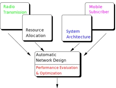
Figure 1: Integrated planning approach
only in a very late stage of the design process. The handling of this issue remains usually to the expertise of the network design engineer.
The demand-based and integrated approach overcomes this disadvantage by regarding the spatial teletraffic demand distribution in the service as a ma-jor input factor among the design constraints. The new approach is depicted in Figure 1. The main cellular design constraints are organized into four equally and parallel considered basic modules, cf. Tutschku et al. [22]: Radio Transmission, Mobile Subscriber, System Architecture, and Resource Man-agement. This structured set of input parameters is used by the integrated concept for the synthesis of a cellular configuration. The system configura-tion is generated by the Automatic Network Design Sequence.
In contrast to the conventional design method, the new approach starts with the analysis of the expected teletraffic demand within the considered
cover-age area, cf. Section 5. Due to the equal and parallel contribution of all basic modules, the new concept is capable to obey the interactions and depen-dencies between the design objectives. Hence, the capacity and teletraffic engineering objectives can be addressed early and in an appropriate way. Moreover, the new approach is able to find trade-offs between contrary ob-jectives, like high user coverage and equipment minimization. It is capable to achieve comprehensive optimized wireless network configurations. Addition-ally, the approach constitutes a forward-engineering technique and facilitates the application of automatic network design algorithms.
3
Traffic estimation
In mobile communication networks the teletraffic originating from the service area of the system can be described mainly by two traffic models which differ by their view of the network. a)The traffic source model, which is also often referred to as themobility model, describes the system as seen by the mobile unit. The traffic scenario is represented as a population of individual traffic sources performing a random walk through the service area and randomly generating demand for resources, i.e. the radio channels. An overview on these models is provided in Section 3.1. b) In contrast, the network traffic model of a mobile communication system describes the traffic as observed from the non-moving network elements, e.g. base stations or switches. This model characterizes the spatial and time-dependent distribution of the tele-traffic. The traffic intensityλis in general measured in call attempts per time unit and space unit ([calls/(sec·km2)]). Taking additionally the mean call
du-rationE[B] into account, the offered traffic isa =λ·E[B] (in [Erlang/km2]). This measure represents the amount of offered traffic in a defined area. Both traffic models are used in mobile communication system design. Par-ticularly the latter model is of principal interest when determining the lo-cation of the main facilities in a mobile network, i.e. the base stations and the switching centers. These components should be located close to the ex-pected traffic in order to increase the system efficiency. Therefore, we focus in Section 3.2 in greater detail on this type of models.
3.1
Traffic source models
Due to their capability to describe the user behavior in detail, traffic source models are usually applied for the characterization of the traffic in an in-dividual cell of a mobile network. Using these models, local performance measures like new call blocking probability orhandover blocking probability
can be derived from the mobility pattern. Additionally, these models can be used to calculate the subjective Quality-of-Service values for individual users.
Overview on traffic source models
A widely used single cell model was first introduced by Hong and Rappa-port [10]. Their model assumes a uniformly distributed mobile user density and a non-directed uniform velocity distribution of the mobiles. Under this premise, performance values like the mean channel holding time and the av-erage call origination rate in a cell can be computed.
A more accurate modeling of the calling behavior of users in a single cell was proposed by Tran-Gia and Mandjes [19]. The model considers a base station with a finite customer population and repeated attempts. The appealing characteristic of the model is the assumption of a small, finite users popula-tion. This is the typical case in real networks, cp. Section 4. However, the model is limited to a single cell and does not consider the spatial variation of the teletraffic within the service area.
El-Dolil et al. [4] characterized the mobile phone traffic on vehicular high-ways by assuming a one-dimensional mobility pattern. They derive the per-formance values by applying a stationary flow model for the vehicular traffic. An extended one-dimensional highway model with a non-uniform density dis-tribution, denoted as the highway PALM model, was investigated by Leung et al. [13]. For the traffic characterization, fluid flow models with time-nonhomogeneous and time-homogeneous traffic have been used, as well as an approximative stochastic traffic model.
A limited directed two-dimensional mobility model was investigated by Fos-chini et al. [5]. The model assumes a spatially homogeneous distribution of the demand and an isotropic mobility structure. Chlebus [2] investigated a mobility model with a homogeneous demand distribution but assumes a non-uniform velocity distribution. The traffic orientation is non-directed and uniformly distributed.
The application of these traffic source models in real network planning cases is strongly limited. Some models, like the highway PALM model give a deep insight on the impact of the terminal mobility on the cellular system
perfor-mance, however they are rather complex to be applied in real network design. Other models, like the one suggested by Hong and Rappaport [10], due to their simplification assumptions, can only be applied for the determination of the parameters in an isolated cell.
3.2
Traffic intensity
Since the cellular network planning process requires a comprehensive view of the expected load and since the traffic source models only focus on a single cell, a network teletraffic model has to be specified. Therefore, we define the traffic intensity function λ(t)(x, y). This function describes the number of call requests seen by the fixed network elements, in a unit area element at location (x, y) during time interval (t, t+ ∆t). The coordinates (x, y) of the area element are integer numbers. Due to the definition given above, the traffic intensity function is a matrix of traffic values representing the demand from area elements in the service region, cf. Figure 2(b). The traffic intensity
λ(t)(x, y) can be derived from the location probability and the call attempt rate of the mobile units.
Under the premise that this probabilityp(t)loc(χ, ψ) is known, the average
num-ber of mobile units #mob(t)(x, y) in a certain area element at timet is:
#mob(t)(x, y) = Z x+∆x x Z y+∆y y p(t)loc(χ, ψ)dψ, dχ . (1)
Here, p(t)loc(χ, ψ) is the probability that, if the system is viewed from the
outside, there is a mobile unit at location (χ, ψ). The location (χ, ψ) is a coordinate in R2 and ∆x×∆y is the size of the unit area element.
Using the assumption that every mobile unit has the same call attempt rate
r(t) at time t, the traffic intensity λ(t)(x, y) can be readily obtained:
λ(t)(x, y) = #mob(t)(x, y)r(t). (2)
Since in real world planning cases it is almost impossible to directly calcu-late the location probability p(t)loc(χ, ψ) from the mobility model, the traffic
intensity has to be derived from indirect statistical measures.
3.3
The geographic network traffic model
The offered traffic in a region can be estimated by the geographical and
demographical characteristics of the service area. Such a demand model relates factors like land use,population density,vehicular traffic, andincome per capita with the calling behavior of the mobile units. The model applies statistical assumptions on the relation of traffic and clutter type with the estimation of the demand. In the geographic network traffic model, the offered traffic A(t)geo(x, y) is the aggregation of the traffic originating from
these various factors:
A(t)geo(x, y) = X
all factorsi ai · δ
(t)
i (x, y), (3)
where ai =λi ·E[Bi] is the traffic generated by factor i in an arbitrary area
element of unit size, measured in Erlangs per area unit, λi the number of
call attempts per time unit and space unit initiated by factor i, E[Bi] is the
mean call duration of calls of type i, and δi(t)(x, y) is the assertion operator:
δi(t)(x, y) =
0 : traffic factor iis not true at location (x, y) 1 : traffic factor iis true at location (x, y)
So far, the planning of public communication systems uses geographic traffic models which have a large granularity. In these cases, a typicalunit area size
is in the order of square kilometers, i.e. in public cellular mobile systems this is the size of location areas, cf. Grasso et al. [8]. For the determination of the location of transmission facilities a much smaller value is required. Their locations have to be determined within a spatial resolution of one hundred meters. Thus, a unit area element size in the order of 100m×100m is here indicated.
Traffic parameters
The values forai, which are the traffic values originating from factoriper area
element, can be derived from measurements in an existing mobile network and by taking advantage of the known causal connection between the traffic and its origin. A first approach is to assume a highly non-linear relationship. A general structure to model this behavior is to use a parametric exponential function. In our proposed geographic model, the traffic-factor relationship is defined to be:
ai =c · bxi (5)
where c is constant andb is the base of the exponential function.
To reduce the complexity of the parameter determination we introduce the normalization constraint:
Atotal
Sservice area/sunit element =
X
all factorsi
ai, (6)
where Sservice area is the size of the service area, sunit element is the size of a unit area element, and Atotal is the total teletraffic in this region. The value of
Atotal can be measured in an operating cellular mobile network.
The structure of the geographical traffic model given in Eqn. 3 and Eqn. 5 appears to be simple. However, due to its structure the model can be adapted to the proper traffic parameters. This capability enables its application for mobile system planning.
Stationary geographic traffic model
The above proposed modelA(t)geo(x, y) includes also the temporal variation of
the traffic intensity in the service area. Since communication systems must be configured in such a way that they can accommodate the highest expected load, the time index t is usually dropped and the traffic models are reduced to stationary models describing the peak traffic. The maximum load is the value of the traffic during the busy hour, cf. Mouly and Pautet [15].
A pitfall for the network designer remains: the busy hour varies over time within the service area. In downtown areas the highest traffic usually occurs during business hours, whereas in suburban regions the busy hour is expected to be in the evening. Therefore, the network engineer has to decide how to weight the different traffic factors, i.e. how to obey the different market shares of various user groups in the traffic model of the network.
3.4
Traffic discretization and demand nodes
The core technique of the traffic characterization proposed in this paper is the representation of the spatial distribution of the demand for teletraffic by discrete points, denoted as demand nodes. Demand nodes are widely used
in economics for solving facility location problems, cf. Ghosh and McLaf-ferty [7].
Definition: A demand node represents the center of an area that contains a quantum of demand from teletraffic viewpoint, accounted in a fixed number of call requests per time unit.
The notion of demand nodes introduces a discretization of the demand in both space and demand. In consequence, the demand nodes are dense in areas of high traffic intensity and sparse in areas of low traffic intensity. To-gether with the time-independent geographic traffic model, the demand node concept constitutes, in the context of cellular network design, astatic popu-lation model for the description of the subscriber distribution.
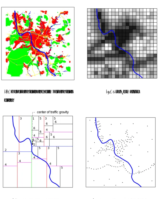
An illustration of the demand node concept is given in Figure 2: part (a) shows publicly available map data with land use information for the area around the city of W¨urzburg, Germany. The information was extracted from
ATKIS, the official topographical cartographical data base of the Bavar-ian land survey office, cf. [1]. The depicted region has an extension of 15km×15km. Figure 2(b) sketches the traffic intensity distribution in this area, characterized by the traffic matrix: dark squares represent an expected high demand for mobile service, bright values correspond to a low teletraffic intensity. Part (d) of Figure 2 depicts a simplified result of the demand dis-cretization. The demand nodes are dense in the city center and on highways, whereas they are sparse in rural areas.
In principle the two-dimensional teletraffic density matrix, cf. Figure 2(b), is sufficient to characterize the teletraffic distribution in the service area.
(a)Geographical and demographical data (b) Traffic matrix 5 2 2 4 4 4 4 3 1 5 3 5 4 4 5 5 3 3 5 5 6 6 6 6 6 6 6 6
center of traffic gravity
(c)Service area tessellation
. ... .. . . .. . . . . ... . . .. . . .. . . .. . .. . . . . . . .. . . . . ... . . . .. . . . . .. . . . . . . . . . . . . . . . . . . .... . . ... . . . .. . . . . . . . .... ....... . . . . . . . . . . . . . . . . . . . . . . . .. .. . .... . . . . . . . .. ..... . . . . . . .. .. . ... .. .... .. . . . ... . .
(d) Demand node distribution
Figure 2: Demand node concept
However, the application of the demand node representation decreases sig-nificantly the computational requirements in network design. Due to the use of discrete point representation, is not necessary any more in mobile
sys-tem design to calculate the field strength at every point in the area. It is adequate to compute the field strength values only at the location of the de-mand nodes, cf. Section 5. Moreover, the discrete presentation can be used to characterize the clustering effect of users in the service area. The demand node concept enables the evaluation of the impact of this user clumping on network performance, cf. Tran-Gia and Gerlich [18].
4
Traffic characterization
4.1
Traffic characterization procedure
Based on the estimation method introduced in the previous section, the traffic characterization has to compute the spatial traffic intensity and its discrete demand node representation from realistic data taken from available data bases. In order to handle this type of data, the complete characterization process comprises four sequential steps:
Step 1 Traffic model definition:
Identification of traffic factors and determination of the traffic parameters in the geographical traffic model.
Step 2 Data preprocessing:
Preprocessing of the information in the geographical and demo-graphical data base.
Step 3 Traffic estimation:
Calculation of the spatial traffic intensity matrix of the service region.
Step 4 Demand node generation:
Generation of the discrete demand node distribution by the ap-plication of clustering methods.
Traffic model definition
The definition of geographical traffic model inStep 1 of the characterization procedure is based on the arguments given in Section 3.3. A simple but accurate spatial geographic traffic model is the base for system optimization in the subsequent network design steps.
Data preprocessing
The data preprocessing in Step 2 is required since the data in geographical information systems are usually not collected with respect to mobile network
4
2
3 1
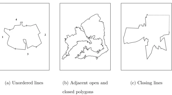
(a) Unordered lines (b) Adjacent open and closed polygons
(c) Closing lines
Figure 3: Original map information data and data preprocessing
planning. For example, ATKIS’ main objective is to maintain map informa-tion. It uses a vector format for storing its drawing objects.
To determine the clutter type of a certain location, one has to identify the land type of the area surrounding this point. This requires the detection of the closed polygon describing the shape of this area. Since maps are mostly printed on paper, the order of drawing the lines of a closed shape doesn’t matter, see Figure 3(a). To identify closed polygons, one has to check if every ending point of a line is a starting point of another one. If a closed polygon has been detected, the open lines are removed from the original base and replaced by its closed representation. Additionally, due to the map nature of the data, two adjacent area objects can be stored by a closed and an open polygon, see Figure 3(b). It also can happen that some data is missing, see Figure 3(c). In this case, line closing algorithms have to applied. After the preprocessing step only closed area objects remain in the data base and the
traffic characterization can proceed with the demand estimation.
Traffic estimation
Step 3 of the traffic characterization process uses the geographical traffic model defined in Step 1 for the estimation of the teletraffic demand per unit area element. The computed traffic values are stored in the traffic matrix. To obtain the traffic value on a certain unit area element, the procedure first determines the traffic factors which are valid for this element and then computes the matrix entry by applying Eqn. 3.
4.2
Demand node generation
The generation of the demand nodes inStep 4 of the characterization process is performed by aclustering method. Clustering algorithms are distinguished into two classes, cf. Jain and Dubes [11]: a)the Partitional Clustering meth-ods, which try to construct taxonomies between the properties of the data points, and b) the Hierarchical Clustering methods which derive the cluster centers by the agglomeration of input values.
The algorithm proposed for the demand generation is a recursive partitional clustering method. It is based on the idea to divide the service area until the teletraffic of every tessellation piece is below a threshold θ. Thus, the algo-rithm constructs a sequence of bisections of the service region. The demand node location is the center of gravity of the traffic weight of the tessellation pieces.
func-Algorithm 1 (Generate Demand Nodes)
variables:
dnode set global variable for the set of generated demand nodes orient orientation of partitioning line
θ traffic quantization value algorithm:
1 procgen dnodes(area, θ,orient = 0) ≡
2 begin
3 if(traffic(area)< θ)
4 thendnode set←center traffic(area);
5 return;
6 elseorient←(orient+ 90o)mod180o; /* turn partitioning line */
7 al=left area(area, orient);
8 ar=right area(area, orient);
9 gen dnodes(al, θ,orient); /* do the recursion */
10 gen dnodes(ar, θ,orient);
11 fi
12 end
Algorithm 1: Demand node generation
tionleft area() divides theareainto two rectangles with the same teletraffic and returns the left part of the bisection. The functionright area() returns the right piece. In every recursion step, the orientation of the partitioning line is turned by 90o. The recursion stops, if every rectangle represents a traffic amount less than the minimal quantization value θ. The function traffic() evaluates the amount of expected teletraffic demand in the area. An example for the bisection sequence of the algorithm is shown in
Fig-ure 2(c). The numbers next to the partitioning lines indicate the recursion depth. To make the example more vivid, not every partition line is depicted in the example. The upper left quadrant of the Figure 2(c) only shows the lines until the recursion depth 3, the lower left part only the lines until depth 4, the lower right quarter the lines until depth 5 and the upper right quadrant lines until depth 6.
The partitional clustering algorithm of Algorithm 1 is a fast but simple clus-tering method. However, its accuracy depends strongly on the quantization valueθ, which gives only an upper bound for the traffic represented by a single demand node. Moreover, since the algorithm constructs a sequence of right-angled bisections, the shape of the tessellation pieces is always rectangular. To overcome these drawbacks, we investigate also hierarchical agglomerative clustering algorithms. These methods are able to obtain tessellation pieces of arbitrary shape and of a predefined traffic value.
5
Automatic cellular network design
5.1
The ICEPT planning tool
To prove the capability of the demand estimation and to show the feasibility of the integrated and systematic design concept,ICEPT (Integrated Cellular network Planning Tool) - a prototype of a planning tool for cellular mo-bile networks was implemented at the University of W¨urzburg, cf. Tutschku et al. [23]. The tools’ core components are the automatic network design algo-rithmSCBPA (Set Cover Base Station Positioning Algorithm), cf. Tutschku [20],
and the traffic characterization procedure as described in Section 4.
The SCBPA algorithm is a Greedy heuristic which selects the optimal set of base stations that maximizes the proportion of covered traffic, i.e. the ratio of the demand nodes which measure a path loss on the forward/reverse link above the threshold of the link budget.
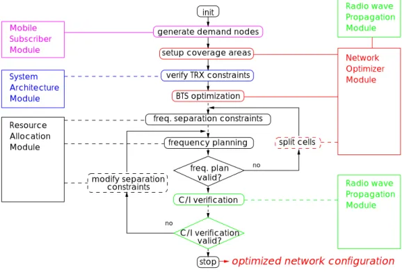
In the ICEPT prototype, the design constraints and objectives are imple-mented as exchangeable modules. These modules are indicated in Figure 4 by the names of the design aspects, like Radio Wave Propagation. ICEPT uses as radio wave propagation models the common Hata model, cf. Hata [9], and the COST231 model, cf. St¨uber [17].
Network Design Sequence
The network design sequence of ICEPT is depicted in Figure 4. In contrast to the conventional cellular design method, the demand-based approach of ICEPT starts with the traffic estimation. Therefore, the tool generates at first the demand node distribution of the planning region. Afterwards, it computes the coverage areas for all potential transmitter locations and con-figurations. In the next step, ICEPT checks whether the traffic and hardware constraints are obeyed at these potential sites or not. Invalid configurations are removed and are not considered in the optimization step. After complet-ing the verification, the SCBPA algorithm generates the cellular configuration by selecting a subset of transmitter configurations from the potential set that maximizes the coverage. The SCBPA algorithm considers during the selec-tion of the transmitters not only the demand coverage, it also minimizes the
Network Optimizer Resource Module Module Mobile Allocation Module Subscriber modify separation constraints split cells
optimized network configuration
freq. separation constraints
frequency planning freq. plan valid? C/I verification valid? C/I verification stop init
generate demand nodes
setup coverage areas
verify TRX constraints BTS optimization no no Radio wave Propagation Module Radio wave Propagation Module System Architecture Module
Figure 4: ICEPT’s network design sequence
carrier-to-interference (C/I) ratios, cf. Tutschku [21]. Subsequently, the tool computes the carrier separation constraints and constructs a frequency allo-cation plan. If the frequency alloallo-cation plan is valid, ICEPT verifies again C/I values of the configuration. In case the C/I constraints are not obeyed, the separation constraints have to be increased. If the C/I specifications are met, the network design stops with the output of the cellular radio network configuration.
5.2
Planning result
ICEPT was tested on the topography around the city center of W¨urzburg. The task was to find the optimal locations of nine transmitters in this terrain.
Figure 5: ICEPT planning result: base station locations
The result of the algorithm is depicted in Figure 5. The base station locations are marked by a diamond-shaped symbol (
). The lines indicate the convex hull around the set of demand nodes which are supplied by the base station. The SCBPA algorithm was able to obtain a 75% coverage of the teletraffic of the investigated area. The total computing time for the configuration, including the traffic characterization, was about 4min on a SUN Ultra 1/170.
6
Conclusion
This paper presented a new model for the characterization of the expected spatial demand distribution in mobile communication systems. The
pro-posed method considers the teletraffic from the viewpoint of the network. Its traffic estimation is based on the geographic traffic model, which obeys the geographical and demographical factors in the service area for the tele-traffic demand estimation. The characterization of the spatial distribution is facilitated by the application of discrete points, denoted as demand nodes. We demonstrated how the demand node pattern can be derived from the information in geographical data bases. Additionally it was outlined how the demand node representation enables the application of demand-based auto-matic mobile network design algorithms.
However, since in practical cellular system design often only rather insuffi-cient geographical and demographical information is available, it would be of great interest to generate demand node patterns artificially by the applica-tion of spatial point processes, like the processes described by Latouche and Ramaswami [12], Stoyan and Stoyan [16], and Cressie [3]. Furthermore, these reference processes could be used to evaluate different planning scenarios.
Future applications of the demand node concept are not limited solely to mobile communication systems. The concept can also be used in other net-work planning scenarios where transmission facilities have to be deployed in a service area, like in wireless access networks, wireline data networks, or
ADSL (Asymmetric Digital Subscriber Line) systems, cf. Maxwell [14]. The demand node concept facilitates a revenue-based system design.
The traffic characterization procedure introduced in Section 4 will soon be available as CUTE (CUstomer Traffic Estimation tool),
http://www.infosim-usa.com/CUTE/
Acknowledgment: The authors would like to thank Titus Leskien, Pe-ter Liebler, and Marius Heuler for their valuable programming support and Michael Wolfrath, Kenji Leibnitz and Oliver Rose for fruitful discussions during the course of this work.
References
[1] ATKIS. Amtliches Topographisches Kartographisches Informations Sys-tem; Bavarian land survey office, Munich, Germany, 1991.
[2] E. Chlebus. Analytical grade of service evaluation in cellular mobile system s with respect to subscribers’ velocity distribution. In Proc. 8th Australian Teletraffic Research Seminar, pages 90–101, 1993.
[3] N. Cressie. Statistic for Spatial Data. Wiley, New York, 1991.
[4] S. A. El-Dolil, W.-C. Wong, and R. Steele. Teletraffic performance of highway microcells with overlay macrocell. IEEE Journal on Selected
Areas in Communications, 7(1):71–78, January 1989.
[5] G. J. Foschini, B. Gopinath, and Z. Miljanic. Channel cost of mobility.
IEEE Transactions on Vehicular Technology, 42(4):414–424, November
1993.
[6] A. Gamst, E.-G. Zinn, R. Beck, and R. Simon. Cellular radio network planning. IEEE Aerospace and Electronic Systems Magazine, (1):8–11, February 1986.
[7] A. Ghosh and S. L. McLafferty.Location Strategies for Retail and Service
Firms. Heath, Lexington, MA, 1987.
[8] S. Grasso, F. Mercuri, G. Roso, and D. Tacchino. DEMON: A forecast-ing tool for demand evaluation of mobile network resources. In Proc. Networks ’96, pages 145–150, Sydney, Australia, 1996.
[9] M. Hata. Empirical formula for propagation loss in land mobile radio services. IEEE Transactions on Vehicular Technology, 29(3):317–325, August 1980.
[10] D. Hong and S. S. Rappaport. Traffic model and performance analysis for cellular mobile radio telephone systems with prioritized and nonprior-itized handoff procedures. IEEE Transactions on Vehicular Technology, VT–35(3):77–92, August 1986.
[11] A. K. Jain and R. C. Dubes. Algorithms for Clustering Data. Prentice Hall, Englewood Cliffs, NJ, 1988.
[12] G. Latouche and V. Ramaswami. Spatial point patterns of phase type. In Proceedings of the 15th International Teletraffic Congress - ITC 15, Washington DC. USA, 1997.
[13] K. K. Leung, W. A. Massey, and W. Whitt. Traffic models for wireless communication networks. IEEE Journal on Selected Areas in Commu-nications, 12(8):1353–1364, October 1994.
[14] K. Maxwell. Asymetric digital subscriber line: Interim technology for th next forty years. IEEE Communications Magazine, 34(10):100–106, 1996.
[15] M. Mouly and M.-B. Pautet. The GSM System for Mobile Communi-cations. published by the authors, ISBN: 2-9507190-0-7, 4, rue Elis´ee Reclus, F-91120 Palaiseau, France, 1992.
[16] D. Stoyan and H. Stoyan. Fraktale — Formen — Punktfelder: Methoden der Geometrie-Statistik. Akademie-Verlag, Berlin, 1992.
[17] G. L. St¨uber. Principles of Mobile Communication. Kluwer Academic Publishers, Boston, 1996.
[18] P. Tran-Gia and N. Gerlich. Impact of customer clustering on mobile network performance. Research Report Nr. 143, University of W¨urzburg, Institute of Computer Science, 1996.
[19] P. Tran-Gia and M. Mandjes. Modeling of customer retrial phenomenon in cellular mobile networks. IEEE Journal on Selected Areas in Com-munications, 15(8):1406–1414, 1997.
[20] K. Tutschku. Demand-based radio network planning of cellular commu-nication systems. InProceedings of the IEEE Infocom 98, San Francisco. USA, 1998. IEEE.
[21] K. Tutschku. Interference minimization using automatic design of cel-lular communication networks. In Proceedings of the IEEE/VTS 48th
[22] K. Tutschku, N. Gerlich, and P. Tran-Gia. An integrated approach to cellular network planning. In Proceedings of the 7th International
Network Planning Symposium (Networks 96), 1996.
[23] K. Tutschku, K. Leibnitz, and P. Tran-Gia. ICEPT - An integrated cellular network planning tool. In Proceedings of the IEEE/VTS 47th
Vehicular Technology Conference, Phoenix. USA, 1997.
[24] P. E. Wirth. The role of teletraffic modeling in the new communication paradigms. IEEE Communications Magazine, 35(8):86–93, 1997.