An Algorithm to Nowcast Lightning Initiation and Cessation in Real-time

An Algorithm to Nowcast Lightning Initiation and

Cessation in Real-time

Valliappa Lakshmanan

, Travis Smith

Abstract

Cloud-to-ground lightning data from the National Lightning Data Network (NLDN), satellite visible and radar-derived products are used to train a light-ning prediction algorithm. The radar reflectivity values are clustered to iden-tify storm and real-time geometric, lagrangian and scalar attributes of those storms are computed. A lightning density field is ”precast” to form the target decision field to be predicted using the computed attributes. Several days of data from the continental United States were chosen to obtain a seasonally and geographically diverse dataset for training. The trained system is used to predict lightning density and the predicted lightning density field is advected to produce a 30-minute nowcast field. The skill of the resulting algorithm is evaluated against a steady-state prediction with motion correction.

1. Introduction

Predicting the spatial and temporal location of cloud-to-ground lightning is a difficult prob-lem. Predicting lightning in time is tied to problems of determining convective initiation. Predicting the location of cloud-to-ground lightning within an electrified storm is subject to knowledge of how lightning travels withins the storm.

Yet, predicting lighting accurately in both space and time is important because light-ning is a potent weather-related hazard. Thus, a short-term (0-1 hour) warlight-ning for in-tense cloud-to-ground lightning has the potential to become a very valuable U.S. National Weather Service product.

∗_{Corresponding author: V Lakshmanan, 120 David L. Boren Blvd, Norman OK 73072;}

A variety of rules of thumb have been developed at various forecast offices to alert the public of the potential of “excessive lightning”. An application to predict lightning, from model forecasts, as an extension of convective activity have been developed, for example by Keller (2004). We, on the other hand, are interested in time frames of less than an hour. Therefore, we formulate the lightning prediction problem as a spatio-temporal predicition problem based on radar-observed inputs. At a particular location, we seek to estimate the probability that there will be a lightning strike at that position in the next 30 minutes. Since lightning is an almost instantaneous event, the probability of lightning is also estimated in a spatio-temporal sense: a particular location is said to have experienced lightning if there is a lightning strike within a given distance of that location within the past 15 minutes. This spatio-temporal defintion of lightning activity is represented by a lightning density grid.

The lightning density grid is a two-dimensional grid that has a resolution of 0.01 de-grees in latitude and longitude (approximately 1km x 1km at midlatitudes). The remapping of lightning source data into lightning density grids is achieved using temporal averaging and spatial smoothing. All the source data that impacts a grid cell over a given time period are used to determine the lightning density at a grid cell. Spatially, we let each source impact not just the grid cell into which it falls, but all grid cells within a given radius (using a Cressman Cressman (1959) neighborhood function to determine the weight of impact). One advantage of cloud-to-ground lightning is that it is a hazard that is observed in real-time. There is no similar real-time source of information on other severe weather hazards such as hail. Thus, it is possible to consider creating a data mining approach to predict cloud-to-ground lightning. If a system can be trained on input spatial grids of reflectivity and VIL at t−30min to predict the cloud-to-ground lightning activity that is

observed at t0, it should be possible to use that system on the set of input spatial grids

at t0 to predict the lightning activity at t30min. Indeed, that was the approach undertaken

by Lakshmanan and Stumpf (2005) where the aforementioned model was created in real-time using radial basis functions which have the benefit of providing a non-linear response while remaining extremely fast to train.

Unfortunately, the approach of using spatial grids directly did not work very well. There were two key reasons. Firstly, storms move. VIL at xi, yi, t−30min was an indicator of

lightning activity not at xi, yi, t0 but at xi +uiδt, yi +viδt, t0 where ui, vi is the motion of

the storm atxi, yi. If that was the only problem, then the target lightning field at t0 could

be advected backwards before training the engine using inputs and outputs at xi, yi. A

second problem is that while reflectivity at−10o_{C was a leading indicator, it was a leading}

indicator of lightning somewhere within the storm, not neccessarily at the location of the overshooting top. In other words, lightning activity was not limited to the core of the storm, but often occured in the anvil region where the radar reflectivity did not overshoot.

input-output mapping has been successfully employed at a 22 km resolution to train a neural network (Burrows et al. 2005). However, at the approximately 1kmresolution that we would like to address, a straight-forward input to output mapping at every grid point will not work. Instead, it is necessary to consider storms as entities and train the model with storm properties, not just pixel values.

2. Method

Cloud-to-ground strike locations from the National Lightning Detection Network (NLDN) were averaged in space (3 km radius) and time (15 minutes) to create a lightning density grid i.e. the value of the grid at any point was an exponentially weighted number of strikes within 15 minutes and 3 km of the point with farther away flashes receiving less weight.

When creating 3D grids of reflectivity from multiple radars (Lakshmanan et al. 2006), we usually map the reflectivity values to constant altitudes above mean sea level. By integrating numerical model data, it is possible to obtain an estimate of isotherm heights – at time intervals of less than an hour, this information is quite reliable. Thus, it is possible to compute the reflectivity value from multiple radars and interpolate it to points not on a constant altitude plane, but on a constant temperature level. This information, updated every minute in real-time, is valuable for forecasting lightning. Following Hondl and Eilts (1994); Watson et al. (1995), we considered the following fields as potential predictors of future cloud-to-ground lightning activity:

1. Reflectivity isotherm values at0o_C,−10o_{C and−20}o_C.

2. Vertical Integrated Liquid (VIL), estimated from multiple radars (Greene and Clark 1972; Kitzmiller et al. 1995).

3. Layer averages of reflectivity between−20o_{C and0}o_C.

4. Maximum VIL and Reflectivity of the storm over its life cycle 5. Increase over time of VIL and Reflectivity isotherms

6. Size and aspect ratio of the storm 7. Speed at which the storm is moving 8. Current lighting density

The motion is estimated using the technique described in (Lakshmanan et al. 2003) and spatial and temporal attributes are extracted using the technique described in (Lak-shmanan and Smith 2008). The t30min lightning density grid was advected backward 30

minutes and used as one of the inputs to the attribute extraction algorithm. These meth-ods are summarized in the rest of this section.

The technique consists of the following steps: 1. identify storms from remotely sensed images 2. estimate the motion of these storms

3. use the spatial extent of the storms and their movement to extract geometric, spatial and temporal properties of the storms

4. In training, use observed lightning density from 30 minutes later advected backwards by 30 minutes as the ”target” or ideal lightning density. Accumulate all such training ”patterns” and train a neural network to carry out the prediction

5. In real-time, provide the geometric, spatial and temporal properties of the storms to the neural network to generate a predicted lighting density. Advect this predicted lighting density field forward by 30 minutes to create nowcast

Extracting storm attributes requires a general-purpose definition of a storm that is amenable to automated storm identification. Lakshmanan et al. (2008) define a storm in weather imagery as a region of high intensity separated from other areas of high in-tensity. A storm in their formalism consists of a group of pixels that meet a size crite-rion (”saliency”), whose intensity values are greater than a value critecrite-rion (”minimum”) and whose region of support (”foothills”) is determined by the highest intensity within the group. The ”intensity” in this case is a multi-radar-derived composite i.e. the maximum radar-observed reflectivity regardless of height at a location. The clustering is set up as an expectation-minimization problem, with two opposing criteria for each pixel so that the cost of assigning a pixel to thekth cluster is:

E(k) =λdm(k) + (1−λ)dc(k) 0≤λ≤1 (1)

The first criterion assigns a cost dm(k) to the difference in intensity between the pixel

intensity (Ixy) and the mean intensity of the kth cluster (µk) so that pixels tend to belong

to the cluster they are closest to in value space: dm(k) =kµk−Ixy kThe second criterion

assigns a costdc(k)defined as the number of neighboring pixels that do not belong to the

kth_{cluster: d}

as their neighbors. Sij is the currently assigned cluster to the pixel ati, j andδis the Dirac

delta function. Thus, the clustering step balances the dual goals of self-similarity (dm(k))

and spatial coherence (dc(k)).

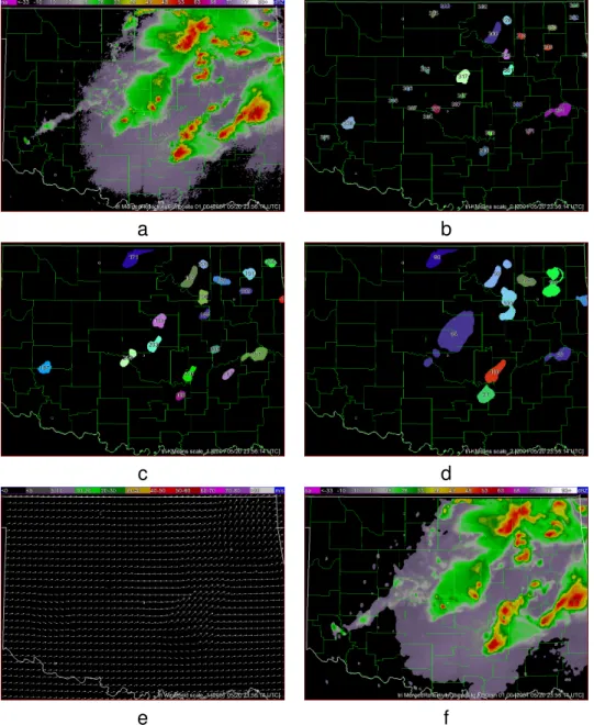
Here, the identification of a storm turns on the size criterion starting from the clusters. These clusters can be combined in descending order of intensity to fit larger and larger size criteria, thus making it possible to use multiple size criteria to achieve hierarchical, multi-scale storm identification (See Figure 1). Doing it this way also yields clusters that are nested partitions, i.e., the storms at more detailed scales are wholly contained within storms at coarser scales.

Clusters identified from the multi-radar composite field at a saliency of 100 km2 _were

used for lighting nowcasting. Lakshmanan et al. (2003) provides a way to obtain high-quality motion estimates, retain the ability to associate motion with storm entities and avoid association error. Storms are identified in the current frame and associated, not with storms in the previous frame, but with the image in the previous frame. Thus, movement is associated not on rectangular subgrids but on subgrids that have the shape and size of the current cluster. Even if a storm has merged or split between the two frames, the motion estimate will correspond to the part of image in the previous frame that the current cluster corresponds to. As long as storms don’t grow or evolve too dramatically in the intervening time period, this cluster-to-image matching side-steps association errors and provides high-quality motion estimates because the motion estimate corresponds to a relatively large group of pixels (See Figure 1e,f). Motion estimates are estimated over the entire area of interest by interpolating spatially between the motion estimates corresponding to each storm. Motion estimates are also smoothed temporally over time using a constant-acceleration Kalman filters. This yields a motion estimate over the entire domain.

Once clusters have been identified and their motion estimated, geometric, spatial and temporal properties of the clusters can be extracted. The number of pixels in each iden-tified cluster is indicative of the size of the cluster. Because the input grids were mapped to an earth-relative coordinate system, the size in pixels can be converted into a size in kilometers.

If the cluster consists of pixelsx, y, then an ellipse can be fit to the cluster’s pixels. The best fit ellipse contains axes of lengthsa andband orientationφwhere Jain (1989):

a= 2qvx+vy+ (vx−vy)2+ 4∗v2xy b= 2qvx+vy −(vx−vy)2−4∗v2xy φ=tan−1 a2/4−vxy (√a2_/4−v x)2+vy2 /_√ vxy (a2_/4−v2 x)2+vxy2 (2)

a b

c d

e f

Figure 1: Multi-scale hierarchical clustering to identify storms and estimate motion. (a) Reflectivity composite field being clustered. The data are over Oklahoma on May 20, 2001 and depict an area of approximately500km×300km(b) Storms identified at a20km2

saliency. Different storms are colored differently. (c,d) Storms identified at 160km2 and

480km2 _{scales. (e) Motion is estimated by matching clusters in the current frame (160km}2

scale shown) to the entire image at the previous image, thus avoiding both association errors and the aperture problem (f) Using the motion estimate to advect the current field foward by 30 minutes

withvx,vy andvxy given by: vx = NΣx 2_−(Σx)2 N2_−N vy = NΣy 2_−(Σy)2 N2_−N vxy = NΣ_Nxy2−Σ_−NxΣy (3)

The ratiomax(a, b)/min(a, b)can be used as a measure of the aspect ratio of the cluster, with a ratio near1indicative of a circular storm and larger numbers indicative of elongated storms.

Multi-radar spatial grids of VIL and reflectivity isotherms are created using the tech-niques described by Lakshmanan et al. (2006). Given a spatial grid of VIL, the maximum VIL within thejth cluster could be expressed as:

V ILclusterj =maxi(V ILxi,yi|xi, yiclusterj) (4)

Thus, spatial properties of thejth_{cluster can be extracted by computing scalar statistical}

properties over all the pixels xi, yi clusterj on spatial grids that have been remapped to

the extent and resolution of the clustered grid.

A potential indicator for lightning initiation/decay is the rate of increase or decrease of VIL. Assume that a motion estimate is available over the entire domain so that the motion atxi, yi is ui, vi. Then, the temporal property that captures the change in a spatial

property, VIL for thejth_{cluster can be obtained by projecting the pixels that belong to the}

cluster backwards in time and recomputing the spatial property on the earlier frame of the sequence:

δV IL,clusterj = maxi(V ILt0,xi,yi|xi, yi clusterj, t0)−

maxi(V ILt−1,xi−ui∗(t0−t−1,yi−vi∗(t0−t−1)|

xi, yi clusterj, t0))

(5)

It should be noted that this technique relies only on the clustering of the current field, and not on the clustering of the previous frame. The assumption, instead, is that the pixels

xi, yi that are part of clusterj will have moved with the same speed and direction from the

previous frame. Therefore, this technique handles morphological operations such as splits and mergers well, since it does not require clustering of the previous frame – instead, just the corresponding part(s) of the previous grid are used. However, this technique assumes that there has not been significant spatial growth or decay of the storm between the time frames. If, for example, there has been decay, then δM ESH,clusterj will reflect only the

changes within the core of the storm (since the cluster att0 will be smaller than the entity

int−1). On the other hand, if there has been growth, then statistics are computed over a

slightly larger area. Because the maximum VIL is typically located well within the core of the storm, this may not matter.

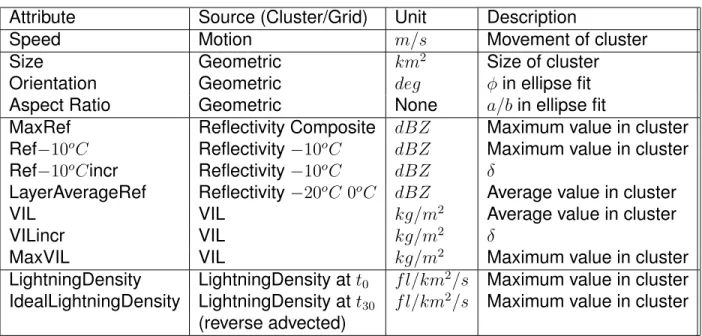
Attribute Source (Cluster/Grid) Unit Description

Speed Motion m/s Movement of cluster Size Geometric km2 Size of cluster Orientation Geometric deg φin ellipse fit Aspect Ratio Geometric None a/bin ellipse fit

MaxRef Reflectivity Composite dBZ Maximum value in cluster Ref−10oC Reflectivity−10oC dBZ Maximum value in cluster Ref−10o_{Cincr Reflectivity−10}o_{C dBZ δ}

LayerAverageRef Reflectivity−20o_{C 0}o_{C dBZ Average value in cluster}

VIL VIL kg/m2 Average value in cluster

VILincr VIL kg/m2 _δ

MaxVIL VIL kg/m2 _{Maximum value in cluster}

LightningDensity LightningDensity att0 f l/km2/s Maximum value in cluster

IdealLightningDensity LightningDensity att30 f l/km2/s Maximum value in cluster

(reverse advected)

Table 1: Attributes extracted from clusters for the lightning prediction algorithm. The units of lightning density are flashes per square kilometer per second.

3. Result

The full list of attributes used for training are listed in Table 1). These were arrived at from the full list of attributes following remove-one feature selection i.e. the full training was carried out after removing one of the features. If the performance of the resulting neural network (on a validation set) did not deteoriate significantly, the feature was permanently removed.

The neural network was trained using spatial (1km resolution every 5 minutes) grids over the continental United States on six days between April and September, 2008: April 10, May 14, June 13, July 1, August 20 and Sep. 111The resulting patterns were randomly divided into 3 sets of 50%, 25% and 25% which were used for training, validation and testing respectively.

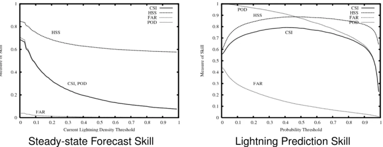
A neural network with one hidden layer consisting of 8 nodes was trained on the train-ing set ustrain-ing ridge regression Riedmiller and Braun (1993), with the validation set utilized for early stopping. The skill of the resulting neural network on the independent test set is shown in Figure 2. If the output of the trained neural network is thresholded at 0.41,

1_{These days were selected because they had relatively widespread lightning activity and because we}

Steady-state Forecast Skill Lightning Prediction Skill

Figure 2: Skill of steady-state method and trained neural network at predicting lightning activity 30 minutes into the future. Critical Success Index (CSI), Heidke Skill Score (HSS), Probability of Detection (POD) and False Alarm Rate (FAR) are shown. The current lightning density field was advected to create ”steady-state” forecasts. The steady-state method has a maximum CSI of 0.69 if the advected field is thresholded at zero. The neural network attains its maximum CSI of 0.79 when its output is thresholded at 0.41.

the algorithm has a Critical Success Index (CSI: Donaldson et al. (1975)) of 0.79 when predicting lightning activity 30 minutes ahead. This corresponds to a Heidke Skill Score (HSS: Heidke (1926)) of 0.89, a Probability of Detection (POD) of 0.91 and a False Alarm Rate (FAR) of 0.14. By way of contrast, simply advecting the current lightning density field and thresholding it at zero attains a CSI of 0.69, HSS of 0.85, POD of 0.71 and FAR of 0.04. The difference in skill is on the order of 0.10 in CSI and can be explained by the ability to predict initiation of lightning (on the order of 0.2 in probability of detection).

In real-time, the neural network can be employed to predict the lightning activity as-sociated with a storm. This probability can be distributed within the extent of the storm and then advected forward in time to yield the probability of cloud-to-ground lightning at a particular point 30 minutes in the future.

The authors are continuing to collect data, and will retrain the system on a year’s worth of geospatial grids (the current training set was limited to the warm season only). At that time, it is expected that testing will be expanded to a larger dataset. Also, it is expected that other forecast time periods (besides the 30 minutes used in this illustration) will be of interest. A clustering saliency of100km2 was arbitrarily chosen here – it is to be expected that a different clustering saliency may provide superior skill and that different forecast

Acknowledgements

Funding for this research was provided under NOAA-OU Cooperative Agreement NA17RJ1227, Engineering Research Centers Program (NSF 0313747).

The attribute-extraction algorithm described in this paper has been implemented within the Warning Decision Support System Integrated Information (WDSSII; Lakshmanan et al. (2007)) as the w2segmotionll process. It is available for download at www.wdssii.org.

References

Burrows, W., C. Price, and L. Wilson, 2005: Warm season lightning probability prediction for Canada and the northern United States.Weather and Forecasting,20, 971–988. Cressman, G., 1959: An operational objective analysis scheme. Mon. Wea. Rev., 87,

367–374.

Donaldson, R., R. Dyer, and M. Kraus, 1975: An objective evaluator of techniques for predicting severe weather events.Preprints, Ninth Conf. on Severe Local Storms, Amer. Meteor. Soc., Norman, OK, 321–326.

Greene, D. R. and R. A. Clark, 1972: Vertically integrated liquid water – A new analysis tool.Mon. Wea. Rev.,100, 548–552.

Heidke, P., 1926: Berechnung des erfolges und der gute der windstarkvorhersagen im sturmwarnungsdienst.Geogr. Ann.,8, 301–349.

Hondl, K. and M. Eilts, 1994: Doppler radar signatures of developing thunderstorms and their potential to indicate the onset of cloud-to-ground lightning.Monthly Weather Re-view,122, 1818–1836.

Jain, A., 1989: Fundamentals of Digital Image Processing. Prentice Hall, Englewood Cliffs, New Jersey.

Keller, D., 2004: Forecasting cloud-to-ground lightning data with AFWA-MM5 model data using the bolt of lightning technique (BOLT) algorithm.Preprints, 22nd Conf. on Severe Local Storms.

Kitzmiller, D. H., W. E. McGovern, and R. F. Saffle, 1995: The WSR-88D severe weather potential algorithm.Wea. Forecasting.,10, 141–159.

Lakshmanan, V., K. Hondl, and R. Rabin, 2008: An efficient, general-purpose technique for identifying storm cells in geospatial images.J. Ocean. Atmos. Tech.,In Press. Lakshmanan, V., R. Rabin, and V. DeBrunner, 2003: Multiscale storm identification and

forecast.J. Atm. Res.,67, 367–380.

Lakshmanan, V. and T. Smith, 2008: Data mining storm attributes from spatial grids. J. Ocea. and Atmos. Tech., Under review.

Lakshmanan, V., T. Smith, K. Hondl, G. J. Stumpf, and A. Witt, 2006: A real-time, three dimensional, rapidly updating, heterogeneous radar merger technique for reflectivity, velocity and derived products.Weather and Forecasting,21, 802–823.

Lakshmanan, V., T. Smith, G. J. Stumpf, and K. Hondl, 2007: The warning decision sup-port system – integrated information.Weather and Forecasting,22, 596–612.

Lakshmanan, V. and G. Stumpf, 2005: A real-time learning technique to predict cloud-to-ground lightning.Preprints, Fourth Conference on Artificial Intelligence Applications to Environmental Science, Amer. Meteor. Soc., San Diego, J5.6.

Riedmiller, M. and H. Braun, 1993: A direct adaptive method for faster backpropagation learning: The RPROP algorithm.Proc. IEEE Conf. on Neural Networks.

Watson, A., R. Holle, and R. Lopez, 1995: Lightning from two national detection networks related to vertically integrated liquid and echo-top information from WSR-88D radar.