Bayesian Variable Selection with Applications to Neuroimaging Data

(1)

Doctoral Dissertations University of Connecticut Graduate School

8-27-2018

Bayesian Variable Selection with Applications to

Neuroimaging Data

Shariq Mohammed

University of Connecticut - Storrs, [email protected]

Follow this and additional works at:https://opencommons.uconn.edu/dissertations

Recommended Citation

Mohammed, Shariq, "Bayesian Variable Selection with Applications to Neuroimaging Data" (2018).Doctoral Dissertations. 1893.

(2)

Applications to Neuroimaging Data

Shariq Mohammed, Ph.D. University of Connecticut, 2018

ABSTRACT

In this dissertation, we discuss Bayesian modeling approaches for identifying brain

re-gions that respond to certain stimulus and use them to classify subjects. We specifically

deal with multi-subject electroencephalography (EEG) data where the responses are

binary, and the covariates are matrices, with measurements taken for each subject at

different locations across multiple time points. EEG data has a complex structure with

both spatial and temporal attributes to it. We use a divide and conquer strategy to build

multiple local models, that is, one model at each time point separately both, to avoid

the curse of dimensionality and to achieve computational feasibility. Within each local

model, we use Bayesian variable selection approaches to identify the locations which

respond to a stimulus. We use continuous spike and slab prior, which has inherent

vari-able selection properties. We initially demonstrate the local Bayesian modeling approach

which is computationally inexpensive, where the estimation for each local modeling could

be conducted in parallel. We use MCMC sampling procedures for parameter estimation.

(3)

complexity parameter built within the model. A prediction strategy is built utilizing

the temporal structure between local models. The spatial correlation is incorporated

within the local Bayesian modeling to improve the inference. The temporal

character-istic of the data is incorporated through the prior structure by learning from the local

models estimated at previous time points. Variable selection is done via clustering of

the locations based on their activation time. We then use a weighted prediction strategy

to pool information from the local spatial models to make a final prediction. Since the

EEG data has both spatial and temporal correlations acting simultaneously, we enrich

our local Bayesian modeling by incorporating both correlations through a Kronecker

product of the spatial and temporal correlation structures. We develop a highly scalable

estimation approach to deal with the ultra-huge number of parameters in the model.

We demonstrate the efficiency of estimation using the scalable algorithm by performing

simulation studies. We also study the performance of these models through a case study

(4)

Applications to Neuroimaging Data

Shariq Mohammed

B.Math.(Hons.), Indian Statistical Institute, 2012 M.Sc., Chennai Mathematical Institute, 2014

M.S., University of Connecticut, 2017

A Dissertation

Submitted in Partial Fulfillment of the Requirements for the Degree of

Doctor of Philosophy at the

University of Connecticut

(5)

Copyright by

Shariq Mohammed

(6)

APPROVAL PAGE

Doctor of Philosophy Dissertation

Bayesian Variable Selection with Applications to

Neuroimaging Data

Presented by

Shariq Mohammed, B.Math.(Hons.), M.Sc., M.S.

Major Co-Advisor Dr. Dipak K. Dey Major Co-Advisor Dr. Yuping Zhang Associate Advisor Dr. Ming-Hui Chen Associate Advisor Dr. Haim Bar University of Connecticut 2018

(7)

Acknowledgments

I would like to extend my deepest gratitude to my advisor Professor Dipak K. Dey

for his constant support and guidance. I am continually impressed by his dedication,

enthusiasm and positivity. Apart from being an amazing advisor, he has also been

extremely supportive of both my academic and non-academic endeavors. I am also

grateful to his wonderful wife, Rita Dey, who has been extremely gracious and helpful.

Both will always remain close to my heart and will be missed.

I would like to thank my co-advisor, Professor Yuping Zhang for supporting and

guiding me, and being very patient throughout my PhD. I would also like to extend my

thanks to my associate advisors, Professor Ming-Hui Chen and Professor Haim Bar for

their insightful suggestions in improving my work. I am grateful to Professor Kun Chen

for motivating and guiding me whenever I sought his help, without any reservations.

I am grateful to the Department of Statistics for all the teaching opportunities and

financial support through fellowships. I thank all the faculty in the department,

espe-cially the ones I have taken courses from, for motivating and kindling my interest in

Statistics. I am fortunate to have interacted with my fellow graduate students, and

heartily thank them for being there throughout this long journey. I also extend my

thanks to Megan, Tracy and Anthony for their cheerful smiles and phenomenal support

(8)

I would also like to acknowledge University of Connecticut and Travelers Insurance,

for supporting the research through grants, both for this dissertation and otherwise.

A special thanks to my teacher, academic brother and friend, Sourish Das, for

be-lieving in my abilities and showing the right direction.

A big thanks to all the friends I have made here, miles away from home. I am

fortunate to have met these awesome people at UConn and will cherish all the moments.

Special thanks to my other friends, in the US and from back home, who have been

there for me through all the times, and dealt with much of my unnecessary ranting, but

still stand by me and let me be myself. I would specifically like to thank Irfan, Ankit,

Debrishi and Aritra for their constant support in both personal and academic fronts.

Lastly, wherever I stand in my career, it is because of the two incredible people

-Shabeer Ahmed (Papaji, my father) and Kausar Banu (Maa, my mother). There are

no words I can use to thank them enough, for all the sacrifices they have made and all

that they have been through, to make me and Shaheer (my brother) the people we are.

I could not have asked for a better person than Shaheer, as a brother. To Maa, Papaji

and Shaheer - I love you and am extremely lucky to have you in my life. I would also

(9)

(10)

List of Tables

1 Simulation results showing the mean prediction error and the average

number of locations selected along with their respective standard

devia-tions - in the case of small mean complexity 0<w <¯ 0.2. . . 35

2 Simulation results showing the mean prediction error and the average

number of locations selected along with their respective standard

devia-tions - in the case of moderate mean complexity 0.3<w <¯ 0.5. . . 35

3 Prediction rates for EEG data. . . 39

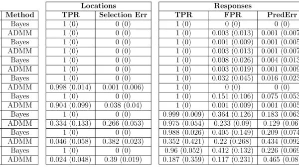
4 Average true positive rate and selection error are shown, along with the

standard error across fifty replications. Error rates for response prediction

are also presented. Results shown for high, medium, and low SNR values

with number of locations as 25. . . 63

(14)

with number of locations as 100. . . 64

7 Error rates from multiple fivefold cross-validations on the EEG data using

local Bayesian modeling approach and the local aggregate modeling (Hu

and Allen [2015]). . . 69

8 Simulation results for the comparison of exact and scalable algorithms

under different settings of L and τ. The average time taken for both

algorithms under each setting is given along with the number of times the

scalable algorithm is faster than the exact one. Mean prediction error on

(15)

List of Figures

1 Example of an EEG cap with electrodes (Source: dreamstime.com). . . . 7

2 |βˆ|for the model withL= 25, τ = 150 andw= 0.5. The panel on the top

shows three parameters whose true values are non-zero and the bottom

panel shows three parameters whose true values are zero. . . 36

3 MCMC samples of the β₂ (L= 25, τ = 150, and w= 0.5) . . . 37

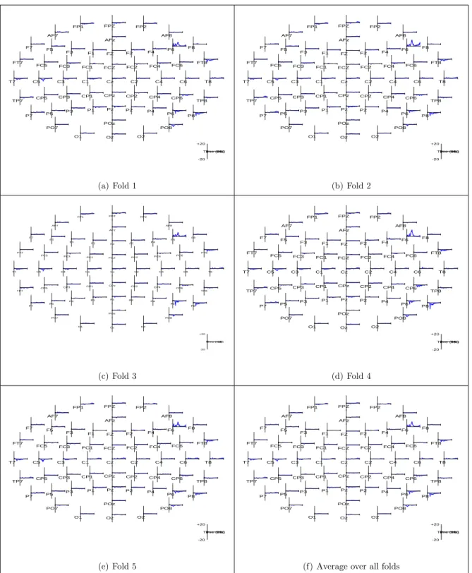
4 Variable selection from local Bayesian modeling using fivefold cross-validation.

The Figures 4(a)-4(e) show ˆβ for each of the five folds. Estimates shown

are obtained using Wcut thresholding method. Figure 4(f) shows the

parameter estimates ˆβ averaged over all five folds. . . 40

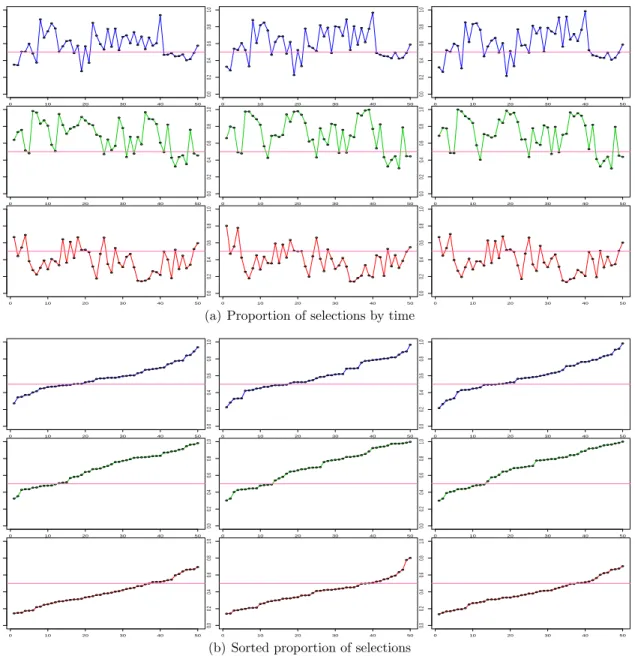
5 Proportion of selectionsp_l are shown in Figure 5(a) as a time series plot

for nine locations across 50 time points. Figure 5(b) shows the sorted

proportion of selections ˜p_l for the same nine locations. . . 56

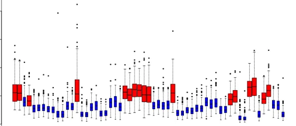
6 Boxplots of observed signal-to-noise ratio for each location and estimates

of coefficients corresponding to locations based on local Bayesian modeling. 68

7 Mean estimated coefficients (not scaled) from local Bayesian modeling

using fivefold cross-validation, shown for the locations which are selected

(16)

8 Estimated local prediction probabilities from a specific fivefold

cross-validation on the EEG data. Each row corresponds to cross-validation data

from one distinct fold. The left (right) column corresponds to subjects

whose true response is y = 1(0). The solid (blue) lines represent ˆy = 1

and the dashed (red) represent ˆy = 0. . . 71

9 Topographic plot of the estimates ˆβ averaged out from each run across

(17)

Chapter 1

Introduction

Recent technological advances in the field of biomedical sciences have led to the

genera-tion of huge amounts of data. It is very common to encounter data with high dimensions,

where the covariates could be matrices or even tensors, instead of the usual vector of

covariates. In such cases, the data has multiple correlation structures acting

simulta-neously and can provide insight into the underlying structure when integrated into the

modeling approaches. With spectacular evolution of data acquisition and storage

facil-ities, along with big memory and computational capabilities of modern technologies, it

is also very often that we encounter the problem of having a huge number of predictors

compared to the observations. With such immense technological advances and

improv-ing capabilities of machines to extract and store huge amounts of data, it has become

necessary to exploit the structure within the data, to develop procedures for efficient

sta-tistical analysis. Handling such massive data to produce meaningful stasta-tistical inference

is a challenge, both in terms of the intricate mathematical modeling by incorporating

the structural information of the underlying biology, as well as the heavy computational

(18)

Among the many statistical applications in the field of biological research, analysis of

the functioning of complex structure of the brain has gained immense importance in the

recent times. There has been a recent trend of promoting interdisciplinary studies for

the science of mind and its realization in biological and artificial systems. Consequently,

the need of neuroscientific, behavioral, and theoretical research in the brain and

cog-nitive sciences has become extremely pertinent. Some of the interdisciplinary research

includes language plasticity, neurobiology of language, dynamical systems science

(mod-eling systems that undergo continuous change), language and logic, philosophy of mind,

evolution of communication, language acquisition, learning, reading, and communication

disorders, neurophysiology, behavioral neuroscience, and molecular genetic neuroscience,

among others.

With fast improving imaging techniques, it is very much feasible to extract data

at extremely granular levels leading to its richness. However, due to the cost involved

with such procedures, we often do not obtain neuroimaging data for a large number

of subjects. This leads to a problem of dealing with ultra-high number of covariates

compared to those of the observations. To address the issue of such high-dimensionality

we are prompted to use efficient modeling procedures incorporating variable selection. In

terms of modeling multi-subject neuroimaging data, variable selection can be interpreted

as spatial clustering of the regions in the brain from where significant electrical activity

emanates. Often, variable selection techniques are used within the modeling to discard

(19)

to understand the underlying process to a large extent. Also, using the covariates to

learn about the characteristics of the observations in the data, is of equal importance.

In this dissertation, we consider a multi-subject neuroimaging data as a motivating

example, where the data is observed for two categories of subjects originating from an

underlying experiment. We address the issue of high-dimensionality by incorporating

variable selection techniques into the modeling. We also use the spatial clustering

gen-erated to be able differentiate between the categories with reasonably high precision,

while still being able to understand the underlying process of the electrical activity. In

section 1.1, we discuss a few variable selection strategies studied in different scientific

applications. We then briefly describe, in section 1.2, the data collection procedure of

electroencephalography along with its structure. In section 1.3 we give an outline of how

the dissertation is organized.

1.1

Variable Selection

Variable and feature selection have taken a center-stage in the areas of application for

which datasets with massive number of covariates are available. Some of these areas

include gene expression analysis, text processing of internet documents, and

combina-torial chemistry, bioinformatics and biomedical studies, among many others. Generally,

the objective of variable selection is threefold: (i) to improve the predictive performance

(20)

provide a better understanding of the underlying process that generated the data. In

the machine learning literature, a lot of approaches have been developed to address

such optimality issues. A basic review of the concepts of feature construction, feature

ranking, multivariate feature selection, efficient search methods, and feature validity

as-sessment methods are given in Guyon and Elisseeff [2003]; and a survey on different

varaible selection algorithms is provided in Chandrashekar and Sahin [2014].

In the context of statistical modeling, one of the crucial questions to address is

the choice of an optimal model from a set of plausible models. When we encounter

significantly higher number of covariates compared to those of the observations (which

is the curse of high-dimensionality with p n), then incorporating variable selection

into the modeling becomes inevitable. One of the most popular techniques called Lasso

was proposed by Tibshirani [1996] which is a penalized least squares method imposing

anL1-penalty on the regression coefficients. As a consequence of usingL1-penalty, lasso

simultaneously obtains both continuous shrinkage and automatic variable selection. This

was later extended by Zou and Hastie [2005] via elastic net, which encouraged grouping

of covariates by facilitating strongly correlated predictors to be in or out of the model

simultaneously. Many other penalized likelihood approaches via regularization are used

for variable selection. Based on the type of penalties considered, efficient algorithms for

estimation have also been developed such as Friedman et al. [2010] and Fan and Li [2001],

among many others. Other dimension reduction techniques such as principal component

(21)

ideal when the interpretation of the statistical inference on individual variable/feature

is relevant in the context of the application.

Instead of directly searching for single optimal model, the task of model selection

in the Bayesian framework is done via parameter estimation. Bayesian variable

selec-tion methodologies usually depend on the properties or characteristics desired from the

model. The degree of sparseness required from the model can be input using an

optimal-ity criterion into the prior, which from a decision theoretic perspective could be viewed as

a loss function (Burnham and Anderson [2002]). Using indicator variables as parameters,

Kuo and Mallick [1998] introduced a Bayesian variable selection approach by

incorpo-rating all possible subsets of predictors to the usual regression equation. Dellaportas

et al. [2002] suggest an alternative model, called Gibbs Variable Selection (GVS), which

extends a general idea of Carlin and Chib [1995] by sampling from a pseudo prior which

has minimal effect on the posterior. Stochastic search variable selection approaches were

introduced through spike and slab priors by George and McCulloch [1993] and extended

to the multivariate case by Brown et al. [1998]. The spike and slab priors were studied

more extensively and extended to rescaled and continuous spike and slab prior by

Ish-waran and Rao [2005]. Other approaches include adaptive shrinkage through Jeffrey’s

prior (Hobert and Casella [1996]) and the Bayesian lasso via the Laplacian shrinkage

(Park and Casella [2008]). Model space approaches include reversible jump Markov chain

Monte Carlo (Green [1995]) and the composite model space (Godsill [2001]). O’Hara

(22)

Bayesian variable selection strategies. Our focus through this dissertation would be on

the spike and slab prior and its variants.

1.2

Electroencephalography (EEG)

Understanding how the human brain works has always been of interest and studied by

scientists, psychologists, and statisticians for a long time. These types of data arise

from various applications in neuroimaging such as magnetic resonance imaging (MRI),

functional MRI (fMRI), electroencephalography (EEG) and magnetoencephalography

(MEG), and other medical imaging procedures such as mammography and ultrasound

imaging. Many attempts have been made for the statistical analysis of such

neuroimag-ing data. Smith and Fahrmeir [2007] use Bayesian variable selection and model averagneuroimag-ing

for a series of regressions located on a lattice. Ising prior is used to spatially smooth the

indicator variables representing whether the variable is zero or not in each regression.

Other recent Bayesian modeling approaches with applications to fMRI data include Lee

et al. [2014]. Based on Bayesian model selection and generative embedding, Stephan

et al. [2017] reviewed single patient analysis and prediction strategies, and developed

generative models for inferring individual disease mechanisms in psychiatry and

neu-rology. Frequentist methods analyzing the data as graphical networks (Ginestet et al.

[2017]) aim at answering questions such as difference in networks between categories of

(23)

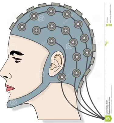
Figure 1: Example of an EEG cap with electrodes (Source: dreamstime.com).

EEG is a noninvasive technology to record the dynamic whole-brain electrical activity,

generated by the synchronized activity of thousands of neurons (in voltage). These

measurements are recorded through the electrodes placed on the scalp surface as shown

in Figure 1. EEG also provides excellent time resolution, allowing us to analyze which

brain areas are active at a certain time. The main objective of EEG is to extract the

spatial and temporal correlations in the brain activity and functional complexity. EEG

analysis has been widely studied as a part of neuroscience, neural engineering, and

clinical studies. Analyzing the electrical activity in the brain caused due to response to

a certain stimulus entails another major challenge of having to deal with low

(24)

A problem of major significance in the study of human brain is the localization of

functional regions in the human brain. Determination of current sources within the brain

is called source localization or the EEG inverse problem. Many scientists in the field of

both clinical and computational neuroscience are interested in addressing this problem.

In terms of statistical modeling, the electrical activity recorded for each subject from

different locations on the brain could be considered as covariates. Since the electrical

activity is recorded at different locations at multiple time points, the subject level

co-variates can be considered as a matrix with an inherent complex correlation structure.

The problem has gained a lot of attention in the neurophysiology and signal processing

community. A survey on the solution of the inverse problem using existing methods in

EEG source localization, is given in Grech et al. [2008] and Jatoi et al. [2014].

Handling such data using classical statistical and machine learning approaches might

be computationally inefficient or might compromise on the correlation structure within

the modeling framework. In such cases, often we have the scenario of p n, due to

which the curse of dimensionality is acute and there are insufficient degrees of freedom

to estimate all the parameters within the model. In multi-subject EEG data, we have

measurements of electrical activity in the brain taken at multiple locations across time,

for each subject. This implies that the subject level covariates are matrices, instead

of vectors, and therefore the multi-subject EEG data is a tensor. Recent statistical

advances have addressed the problem of handling tensor data. Zhou et al. [2013] have

(25)

the covariates by reducing the ultra-high dimensionality to a manageable level. More

recently, classification problems have been addressed through logistic tensor regression

by Tan et al. [2012], with applications to facial image recognition and motion data.

However, in this dissertation, to analyze such high-dimensional and structural data, we

discuss a Bayesian approach. We use a divide and conquer strategy to build multiple

models to achieve computational efficiency. Specifically, in the case where p n, it

is appealing to incorporate Bayesian strategies as it combines prior information with

the data, within a decision theoretic framework. Small sample Bayesian modeling also

provides inferences that are conditional on the data and are exact, without reliance

on asymptotic approximation. To address the problem of identifying the active brain

regions is analogous to doing variable selection or spatial clustering of different regions

of the brain.

The data we consider throughout this dissertation arises from a large study to

exam-ine EEG correlates of genetic predisposition to alcoholism. Electrical activity is measured

through electrodes placed on the scalps of the subjects which were sampled at a high

fre-quency. Two groups of subjects, alcoholic and control were exposed to pictures of objects

as visual stimuli from the Snodgrass and Vanderwart [1980] picture set. The data

collec-tion process is described in more detail in Zhang et al. [1995]. The complete version of the

data set is publicly available at https://archive.ics.uci.edu/ml/datasets/eeg+database.

We mainly work with the cleaned version of this dataset provided in the supplementary

(26)

1.3

Dissertation Outline

In this dissertation, we address the problem of understanding the extremely complex

structured EEG data through Bayesian approaches. We incorporate variable selection

strategies into the prior structure to identify the regions of interest in the brain. We also

deal with the computational complexity issues by using divide and conquer strategies

within the modeling to make the estimation and inference feasible.

In Chapter 2, we present a Bayesian variable selection method to identify the active

regions in the brain as a response to a certain stimulus. We build binary classification

models of subject-level responses using binary regression with Gaussian models on the

latent variables. We also study the scaled normal priors on the latent variables, as they

cover a large family of distributions. We use the continuous spike and slab priors to

in-corporate variable selection within the modeling. Due to the computational complexity,

we build many local (at different time points) models and make predictions by

utiliz-ing the temporal structure between the local models. We perform a two-stage variable

selection for each of these local models. We demonstrate the effectiveness of such

model-ing through the results of a simulation study. We then present the performance of these

models on multi-subject neuroimaging (EEG) data to study the effects on the functional

states of frontal cortex and parietal lobe for chronic exposure of alcohol. We also discuss

(27)

In Chapter 3, we develop a similar Bayesian approach for the analysis of

high-dimensional neuroimaging data. Unlike the assumptions in Chapter 2, we incorporate

spatial correlation structures within the modeling to improve the inference. We

specifi-cally deal with EEG data, where we have a matrix of covariates corresponding to each

subject from either the alcoholic or control group. The matrix covariates have a natural

spatial correlation based on the locations of the brain. We employ a divide and

con-quer strategy by building multiple local Bayesian models at each time point separately.

We incorporate the spatial structure through the structured spike and slab prior, which

has inherent variable selection properties. We also have temporal correlation within the

covariates as the measurements are taken over time. This temporal structure is

incor-porated within the prior by learning from the local model from the previous time point.

We pool all the information from the local models and use a weighted average to design

a prediction method. We perform some simulation studies to show the efficiency of our

approach and demonstrate the local Bayesian modeling with a case study on EEG data.

We also discuss some crucial advantages of using the local modeling approach on such

high-dimensional data with low signal-to-noise ratio.

Motivated by the results from the local Bayesian modeling in Chapter 2 and 3, we

further develop the modeling strategies. In Chapter 2 we have an appealing

compu-tational advantage of estimating the local models in parallel. Whereas in Chapter 3,

having incorporated the spatial correlation, we learn from the local model at previously

(28)

same problem of binary classification of neuroimaging data with matrix valued

covari-ates, but we now incorporate both spatial and temporal correlations simultaneously

within the local Bayesian modeling approach. The spatio-temporal correlation structure

is incorporated through the Kronecker product of the spatial and temporal covariance

structures into the continuous spike and slab prior. We then address the computational

complexities arising from such modeling structure to achieve feasible estimation

proce-dures. We develop a highly scalable estimation procedure based on MCMC sampling

to completely avoid large matrix inversions and huge sequential estimations. The

scal-ability is achieved by incorporating a likelihood approximation and predictive inference

strategy within the sampling procedure. We describe both the exact estimation using

Gibbs sampling and the scalable estimation algorithms. We then do a simulation study

to compare the performance of the exact and scalable algorithms in terms of variable

se-lection, prediction and computation time. The main advantage of the scalable algorithm

is that the computation time is reduced, as the computations for all the spatio-temporal

parameters need not be done sequentially, which would be the case if we used the

ex-act estimation algorithm. We then use the spatio-temporal modeling along with the

scalable estimation algorithm to study a multi-subject neuroimaging data through an

EEG case study. We draw comparisons of the results based on independent local

mod-eling from Chapter 2, the spatial structured local modmod-eling from Chapter 3, and the

spatio-temporal modeling of Chapter 4. We end the dissertation with a discussion, some

(29)

Chapter 2

Local Modeling of EEG Data Using

Continuous Spike and Slab Prior

2.1

Introduction

In this chapter, as a motivating example, we deal with multi-subject neuroimaging data

through a case study on electroencephalography (EEG), one of the popular noninvasive

brain-imaging techniques which monitors electrical activity in the brain. The main

ob-jective of EEG analysis is to extract information from brain in a spatio-temporal pattern

and learn about the functional connectivity between different brain areas as a response

to certain stimulus. Understanding such patterns through an automated procedure is

of extreme importance in many areas of neuroscience research, including in the study of

neurophysiological oscillations associated with normal brain functions and the changes

in these processes caused by diseases or through interventions. This understanding is

also crucial in the development of brain-computer interfaces and clinical investigations.

(30)

and high-dimensionality pose great challenges in building efficient statistical models.

We focus on identifying brain regions associated with the response to a certain

stim-ulus, by classifying the disease status based on the neuroimaging data. There have

been several methods proposed to handle data where the subject-level covariates are

matrices. The most common approach to handle such data is by vectorizing the matrix

of covariates, which clearly lands us into a high-dimensionality problem. Voxel-based

methods (Worsley et al. [2004]) have been proposed, where the image data at each voxel

is considered as a response and clinical variables as predictors, to generate a statistical

parametric map of test statistics or p-values across all voxels. Another approach (Caffo

et al. [2010]) is to first reduce the dimensions through methods such as principal

compo-nent analysis (PCA) and then fit the models based on the reduced dimensions obtained.

However, it is well known that the dimensions obtained through PCA might not be easily

interpretable. Several frequentist approaches have proposed regularization methods for

matrix GLMs by using low-rank constraints, penalties or low-rank structured coefficient

models (Zhou et al. [2013], Zhou and Li [2014]) or placing two-way penalties on the

covariance matrix (Tian et al. [2012]) or local aggregate modeling using spatio-temporal

penalties (Hu and Allen [2015]). In this chapter, we discuss a Bayesian approach to

ana-lyze such high-dimensional data by exploiting its inherent structure, using a divide and

conquer strategy to build multiple models with computational efficiency. Bayesian

anal-ysis combines prior information with the data in a natural and principled way, within

(31)

analogous to that of doing variable selection or spatial clustering on the regions. We

will use one of the popular variable selection priors - continuous spike and slab prior

(Ishwaran and Rao [2005]) to incorporate variable selection within our modeling setup.

In section 2.2, we introduce the notation we use, discuss the structure of the data in

detail, and give a brief overview of our modeling strategy. In section 2.3, we begin our

analysis by considering the local aggregate modeling (Hu and Allen [2015] and discuss its

interpretation from a Bayesian perspective, along with its computational challenges. In

section 2.4, we propose local Bayesian modeling using the spike and slab prior (Ishwaran

and Rao [2005]). We consider normal prior (section 2.4.1) on the latent variable in the

model and then extend it to scale mixture of normal priors (section 2.4.2). We also

discuss the parameter estimation using Gibbs sampling along with the advantages of our

modeling setup. In section 2.5, we propose a two-stage variable selection strategy where

the first stage variable selection is done by thresholding and the second stage by analyzing

the consistency of selections from the first stage. Our prediction method, as described

in section 2.6, incorporates the temporal pattern within the modeling framework. In

section 2.7, we show the results from a simulation study where we test the performance

of our models for varying number of parameters (across both the dimensions of the

covariates). In section 2.8, we apply our local Bayesian modeling to the multi-subject

neuroimaging data through a case study on the EEG data, and present our analysis

of the reaction of the brain regions to visual stimulus. In section 2.9, we give a short

(32)

2.2

Data and Notation

We start with some notation which we will use throughout this dissertation. We denote

tensors by X, matrices by X, vectors by x, and scalars by x. Let vec(X)∈_Rnp _{be the}

vectorized version ofX∈_Rn×p_{, and let the matricized version of the tensor}_X _∈

Rn×p×q

be written as X(1) ∈Rn×pq along the first mode and similarly for other modes.

Let y ∈ {0,1}n _{be the vector of subject-level binary responses. For} _n _independent

subjects, L locations on the brain and τ time points, let Xn×L×τ be the tensor of pre-dictors from the EEG data. These prepre-dictors are continuous variables as EEG measures

the change in voltage resulting from ionic current within the neurons of the brain.

An elementary approach is to start by assuming that (y,X) follows a matrix gen-eralized linear model (matrix GLM) as g(µ) = α+X(1)vec(B), where µ =E(y|X) is

the conditional mean response,g(.) is the canonical link function,α∈_Ris the intercept

term, and the coefficient matrix given asB= [β₁, . . . ,β_L]∈_Rτ×L_{. Unfortunately, these}

matrix GLM models are ultra-high dimensional statistical problems where n is of the

order of tens or hundreds and Lτ is of the order of tens of thousands to even millions,

creating a pn situation.

To achieve computational efficiency of the algorithm, Hu and Allen [2015] propose

local aggregate modeling approach, which shall be discussed in section 2.3. In the local

aggregate modeling, GLMs are fit at each location separately and then an ensemble

(33)

model at any location, the number of covariates corresponding to each subject would

be τ. The number of time points at which the measurements are collected in the EEG

data could be very large compared to the number of subjects, as it depends on the

frequency used during the data collection process. For example, if the data is collected

at a frequency of 256 Hz for a duration of 5 seconds, then we would have a total of

256 ×5 = 1280 measurements for each location and each subject. In contrast, even

the high-density EEG sensors do not have more than a couple of hundreds of channels

(locations). Hence, we propose to build local models at each time point separately, where

the subject-level covariates for each local model would be the measurements at different

locations at that particular time point, as shown in (2.2.1). That is, we use Xt ∈Rn×L

as the covariates at time pointt. We then incorporate the variable selection through the

prior structure within our local Bayesian modeling.

response z }| {          y1 .. . yn          n×1 ∼ Time 1 z }| {          X1          n×L   β1    L×1 Time 2 z }| {          X2          n×L   β2    L×1 . . . Timeτ z }| {          Xτ          n×L   βτ    L×1 (2.2.1)

(34)

2.3

Local Aggregate Modeling Extension

In the local aggregate modeling approach (Hu and Allen [2015]), one models the

multi-subject binary response vector from the EEG data at each location separately through

local GLMs: g(µ_l) = αl+Xlβl, ∀l = 1, . . . , L, where Xl ∈Rn×τ is the data at location

l,µ_l=E(y|Xl) is the local conditional mean andαl is the local intercept. An ensemble

of these local models is built using the regularization

min α,B L X l=1 h l(y;αl+Xlβl) +λ sm locβ T l Ωβl+λ sp loc||βl||2 i +λaggtr(BGBT), (2.3.1)

whereΩ is the second order difference matrix penalizing the squared distances between

coefficients at adjacent time points, G=D−W is the Laplacian matrix with D as the

degree matrix for the locations and W as the adjacency matrix of the weights assigned

to the edges between two connected locations. The quantities λsm_loc, λsp_loc and λagg are the

tuning parameters for local smoothing, local separability, and aggregation respectively

and ||.||2 denotes theL2-norm. The term

L P l=1

||β_l||2 treats coefficients at each location as

a group and zeros out all elements of β_l and is similar to group lasso, as it is separable

in locations.

We now consider the penalty terms in the minimization problem in equation (2.3.1)

(35)

from a Bayesian perspective. For the location penalty, we have L X l=1 λsm_locβT_l Ωβ_l+λsp_loc||β_l||2 = L X l=1 βT_l λsm_locΩ+λsp_locIτ β_l, where (λsm locΩ+λ sp

locIτ) is clearly a positive definite matrix (hereIτ is the identity matrix of dimensionτ). From a Bayesian perspective, this can be thought of as having Gaussian

priors on β_l such that

β_liid∼ N 0,(λ_locsmΩ+λsp_locIτ)−1

, ∀ l = 1, . . . , L. (2.3.2)

For the aggregation penalty, we have (see Appendix A.1)

L X l=1 λaggtr(BGBT) = 1 2 τ X t=1 βT_t. λagg(D−W) β_t.,

where for each t = 1, . . . , T, βT_t. = (β_t₁, . . . ,β_lt) is the vector of coefficients from B

corresponding to time point t, N(l) is the set of all neighbors of the location l, and

G = D−W is the Laplacian matrix as mentioned earlier. G is positive semidefinite,

which restricts us from considering independent Gaussian priors on β_t..

We could address this by adding an extra separability penalty term in (2.3.1) for the

aggregation part, which would then make it

L X l=1 λsm_aggtr(BGBT) + τ X t=1 λsp_agg||β_t.||2 = τ X t=1 βT_t.(λsm_aggG+λsp_aggIL)β_t.,

(36)

where λsm_agg and λsp_agg are the tuning parameters for smoothing and separability (similar

to what we had for locations earlier) in the temporal dimension respectively. The matrix

(λsm

aggG+λspaggIL) is positive definite whenIL is the identity matrix of dimension L, and we can consider it as a prior on time points as follows:

β_t. iid∼N 0,(λ_aggsmG+λsp_aggIL)−1

, ∀t = 1, . . . , τ. (2.3.3)

The prior specifications given in (2.3.2) and (2.3.3) are essentially priors on the

columns and rows of the coefficient matrix B. In (2.3.2), if the locations are

indepen-dent, then the temporal structure is exploited using a second order difference matrix

Ω. Similarly, assuming independence across the time points in (2.3.3), the spatial

de-pendence between locations is exploited. These can be implemented as simple Gaussian

priors to do the estimation. But these priors just by themselves do not possess any

variable selection properties. Owing to the large number of locations or time points, we

are motivated to use priors with inherent variable selection properties. The structure

of connections in the human nervous system is extremely complex, and we might not

always have access to the degree matrix D and adjacency matrix W, in which case

the number of parameters to estimate increases rapidly. With these considerations, we

propose a hierarchical Bayesian model using spike and slab priors in the next section.

Spike and slab priors have inherent variable selection properties, where each component

(37)

2.4

Spike and Slab Prior with Latent Variable

In the EEG data described in section 2.2, the number of subjects n is of the order of

hundreds whereas, the number of predictors Lτ is of the order of tens of thousands. If

we consider a Bayesian model with y as the binary response variable and X(1) as the

n ×Lτ matrix of predictors, then we encounter the problem of Lτ n. In such a

case, Bayesian modeling for variable selection has limitations as it is computationally

infeasible to visit all 2Lτ models in the MCMC chain.

To surpass the Lτ n issue, we propose local Bayesian modeling, which fits local

models at each time point separately. As our response is binary, we use latent variable

regression (Albert and Chib [1993]) with spike and slab prior on the coefficient vectors.

Let us denote Y = [y₁, . . . ,y_τ] ∈ {0,1}n×τ _{as the matrix of the collection of response}

vectors and Z = [z1, . . . ,zτ] ∈ Rn×τ as the matrix of latent vectors, where yt is the

response vector at time point t and zt is the latent variable vector corresponding to

the time point t. Although we use the notation y_t for the binary response vector at

time point t, note that y₁ = y₂ = . . .=y_τ. In this section, we propose local Bayesian

modeling with normal link as well as scale mixture of normal link on the latent variable.

The scale mixture of normal link covers a wide variety of family of distributions, of

which normal link would become a special case. In particular, we consider the Student’s

(38)

2.4.1

Normal Link

For each time point t ∈ {1, . . . , τ} and for each i= 1, . . . , n, we defineyit = 1 if zit >0

and yit= 0 otherwise. If the zt are modeled as

zt|βt∼N(Xtβt,In), (2.4.1)

then it can be easily shown that yit are independent Bernoulli random variables with

pit = P(yit = 1) = Φ(xTitβt), where xTit is the ith row of the matrix Xt and Φ(.) is

the cumulative distribution function of standard normal distribution. We now consider

the spike and slab prior (Ishwaran and Rao [2005]) on the coefficient vector βT_t =

(β1t, . . . , βLt) as follows: βlt|ζlt, νlt2 ind ∼ N(0, ζltνlt2) (2.4.2) ζlt|v0, wt iid ∼ (1−wt)δv0(.) +wtδ1(.) (2.4.3) ν_lt−2|a1, a2 iid ∼ Gamma(a1, a2) (2.4.4) wt ∼ U(0,1), (2.4.5)

where ζltνlt2 is the hypervariance with ζlt as an indicator taking one of the two values

1 or v0. For a real number c, δc(.) is the discrete measure concentrated at c. Here,

v0 (a small quantity near zero), a1 and a2 (shape and rate parameters of a gamma

(39)

spike at v0 and a right-continuous tail (Ishwaran and Rao [2005]). The parameter wt is

the complexity parameter dealing with the size of the models (which is the number of

nonzero coefficients inβ_t). Its value controls the probability ofβltbeing chosen (ζlt= 1)

or not (ζlt=v0).

Let ζT_t = (ζlt, . . . , ζlt), ν−t2 T

= (ν_lt−2, . . . , ν_tl−2) and assume γlt = ζltνlt2. Let Γt =

diag(γ_t), where γT_t = (γ1t, . . . , γLt). See Appendix A.2 for the posterior density of

zt,βt,ζt,ν

−2

t and wt. Given yt (note that yt = y for all t ∈ {1, . . . , τ}), the full conditional distributions of zit,βt, ζlt, νlt−2 and wt are given as:

1. zitare independent withzit|βt ind

∼ N(xT_itβ_t,1) truncated at the left by zero ifyit= 1,

and zit|βt ind

∼ N(xT

itβt,1) truncated at the right by zero if yit= 0.

2. β_t|zt,γt∼N(ΣtXTtzt,Σt), where Σt= (XtTXt+Γ−t1) −1_. 3. ζlt|βlt, νlt2, wt ind ∼ w1,l,t w1,l,t+w2,l,tδv0(.) + w2,l,t w1,l,t+w2,l,tδ1(.), where w1,l,t= (1−wt) 1 √ v0 exp− β 2 lt 2v0ν_lt2 and w2,l,t =wt exp − β 2 lt 2ν2 lt . 4. ν_lt−2|βlt, ζlt ind ∼ Gammaa1+1₂, a2 + β2_lt 2ζlt . 5. wt|(ζ1t, . . . , ζLt)∼Beta 1 + #{l|ζlt = 1},1 + #{l|ζlt =v0} .

We see that the posterior distributions of all the parameters are from standard

distribu-tions and hence we can use Gibbs sampling for the estimation within each local model.

(40)

4 and 5 as numbered above. We start withβ_tequal to the parameter estimate from a

lo-gistic regression model whenXtis regressed ony. For a few time points, the coefficients

might yield a singular covariance structure of posterior distributions within the MCMC

chain. For such time points, we start with the initial value of β_t as a zero vector. We

choose an initial value for the complexity parameter as w_t(0) and the initial value ofζ_t is

generated asL independent samples from a discrete distribution which generates 1 with

probabilityw(0)_t and v0 with probability 1−w (0)

t . The initial value ofνlt2 is chosen as the mode of its prior distribution which is a2/(a1 + 1), wherea1 >2 for all l = 1, . . . , L.

2.4.2

Scale Mixture of Normal Link

By introducing latent variables, the probit regression on the binary response vector y_t

has an underlying normal regression on zt. To incorporate heavier tails in the prior

specification for the latent vector in (2.4.1), instead of a normal link we consider the

scale mixture of normal link

zt|βt,Ct∼N(Xtβt,Ct), (2.4.6)

where Ct = ctIn with ct as the scaling factor. If the scaling factor is fixed, the full

conditional distributions of zit and βt are given as

• zit are independent with zit|βt, ct ind

∼ N(xT

itβt, ct) truncated at the left by zero if

yit = 1, and zit|βt, ct ind

∼ N(xT

(41)

• β_t|zt,γt∼N(ΣtXTtC

−1

t zt,Σt) where Σt = (XTtC

−1

t Xt+Γ−t1)−1.

The full conditionals of the other parameters remain the same as in the normal link case

in section 2.4.1.

Now let us consider ct as an arbitrary scaling factor, and consider the prior c−t1 ∼

Gamma(q₂,q₂), where q₂ is the value for the scale and rate parameters of gamma density.

The full conditionals of zlt,βt, ζlt, νlt−2 and wt are the same as the full conditionals of

these parameters in the fixed scaling factor case. The full conditional distribution of ct

is given by c−_t1|zt,βt∼Gamma n+q 2 , q 2+ 1 2 n P i=1 [zit−xTitβt]2

. The Gibbs sampler for the

scale mixture of normal prior is implemented in a similar way as for the normal prior.

We start with the same initial values as in the normal prior case. Here, the initial value

of Ct can be considered as the identity matrix In.

It is well-known that considering the prior distribution on the latent variable as

zit|βt, ct ∼ N(xTitβt, ct) with a prior on the scaling factor as c

−1 t ∼ Gamma( q 2, q 2) is

equivalent to having the prior zit|βt ind

∼ tq(xTitβt,1) that gives a link function from

Stu-dent’stdistribution withqdegrees of freedom andxT

itβtas its location parameter. There are several advantages of considering t link in the model. It provides flexibility in

mod-eling: by varying the degrees of freedom (heavy or thin tailed), we can choose the value

for q which supports the data better. Also, a Student’st distribution with appropriate

degrees of freedom approximates a logistic distribution (Mudholkar and George [1978],

Kim et al. [2007]). Hence, we can also compare the performance of the model under a

(42)

Let us consider the prior on the scaling factor with different scale and rate

param-eters, such as c−_t1 ∼Gamma(q1

2, q2 2), where q1 2 and q2

2 are the scale and rate parameters

of gamma density, respectively. This prior on the scaling factor in conjunction with

zit|βt, ct∼N(xTitβt, ct) as the prior distribution on the latent variables, is equivalent to

having a generalized t-distribution (Arellano-Valle and Bolfarine [1995]) with q1 as the

shape parameter or degrees of freedom,q2 as the scale parameter andxTitβtas its location

parameter. When the scale and rate parameters are the same, i.e., when q1 = q2 = q,

then we have a Student’s t-distribution as a special case of a generalized t-distribution,

as seen before. For a binary response dataset, if the probability approaches 0 or 1 at a

faster rate than a probit link, then a generalized t-link may fit the data better than a

Student’s t-link. In section 2.7 and 2.8, we shall present results corresponding to t-link.

2.5

Two-Stage Variable Selection

We fit local Bayesian models for each time point as specified in section 2.4. Note that

we can obtain exact zero coefficients when we use the frequentist variable selection

approaches via regularization. However, when we use MCMC methods to obtain samples

from posterior distributions, we do not obtain exact zero estimates after shrinkage. In

this section, we discuss thresholding criteria for estimates from our Bayesian model. If

the covariates of local models at each time point are locations, then thresholding the

(43)

We propose a two-stage variable selection strategy as follows: (i) by using thresholding

methods in the first-stage to force point estimates with smaller magnitudes to zero, and

(ii) in the second-stage, we analyze the spacings of the binary sequence obtained from

the first-stage to determine the final selection of locations.

2.5.1

First-Stage Variable Selection

In our problem, we focus on the estimation of theβ_t, which are the parameter estimates

corresponding to the locations. As the posterior distribution of β_t is a multivariate

normal distribution, we consider its posterior mean ˆβ_t as the estimate of β_t and

appro-priately threshold them to do the variable selection. The posterior mean obtained using

the spike and slab prior shrinks the null coefficients, while the larger coefficient values

are retained with higher magnitude. We could consider different thresholds to obtain

the final estimates. For the rescaled spike and slab model, as described in Ishwaran and

Rao [2005], the Zcut method, which is a hard shrinkage rule, is considered as a threshold

rule to force the coefficients to be zero. They also show that, when compared with OLS,

the Zcut method has an oracle like misclassification property. In the Zcut method the

coefficients are set to zero by treating the posterior mean values as N(0,1) statistics

and comparing them with appropriate thresholds from a standard normal distribution.

Using the formal definition (Ishwaran and Rao [2005]), the Zcut estimates (the set of

(44)

β_tZ ={βˆlt:|βˆlt|> zα/2}, (2.5.1)

where ˆβ_t = ( ˆβ1t, . . . ,βˆLt) are the posterior mean estimates from the spike and slab model,

α is a fixed user-specified value and |.| denotes the absolute value. All the remaining

coefficients which do not pass the criteria in (2.5.1) are set to zero.

Taking a cue from the Zcut method, we formulate another way of thresholding using

ˆ

wt, the posterior mean of the complexity parameterwt. We rank the posterior means ˆβt

in the decreasing order of their absolute values and choose the first bLwˆtc coefficients as

the nonzero coefficients and set the rest of them to zero. We refer to this as the Wcut

method where the coefficients are set zero or nonzero as follows:

βW_t ={βˆlt: rank |βˆlt|

<bLwˆtc}, (2.5.2)

where rank(xi) is the rank of xi, and bxcdenotes the floor function. If a predetermined

constant is used as a threshold, then the set of nonzero coefficients are βC_t = {βˆlt :

|βˆlt|> k}. We refer to it as the Ccut thresholding criteria, of which the Zcut method is

a special case.

Using any of the above thresholding methods, at each time point t, we obtain a set

of variables with nonzero coefficients and the rest of the variables are set to zero. When

the covariates are locations, these two sets of coefficients can be considered as a spatial

(45)

different spatial clusters for each of those local models. That is, the set of variables

selected by local models might not be the same across all the time points, as the signal

in the data might not remain throughout the duration, and the brain regions responding

to a stimulus might change with time. Hence, we propose to use the union of all the

variables selected for each of the local models. After fitting the spike and slab model for

each time point, the set of covariates selected by Zcut, Wcut, and Ccut in the first-stage

variable selection are given by βZ, βW, and βC respectively, where

βm =βm₁ ∪βm₂ ∪. . .∪βm_τ with m =Z, W, or C. (2.5.3)

Because of the large number of time points, taking a union of locations selected at each

time point might not be very efficient. We resort to a second-stage of variable selection

using the selection information of locations from the first-stage. We analyze the pattern

of selection of each location to determine its final selection status.

We shall present our simulation results for both Zcut and Wcut thresholding

meth-ods. For brevity we will consider Wcut as our thresholding method for the first-stage

variable selection throughout this chapter, unless specified otherwise.

2.5.2

Second-Stage Variable Selection

After the first-stage variable selection, coefficients of each location can be looked at as a

(46)

selected by the local model at time t and ˆβlt 6= 0 indicates selection. For each location

we can consider a binary sequence of indicators across all time points. We analyze the

spacings of this binary sequence (Albert [2013]) to perform the second-stage variable

selection. Consider a binary (0 or 1) sequence of indicators withR ones in the sequence

and the rest zeros. For simplicity of notation, let us assume that for some location,

the spacings e1, . . . , eR+1, denote the number of times that location was not selected

between two consecutive selections. We consider a Bayes factor test statistic by modeling

er with a geometric distribution. We assume that e1, . . . , eR+1 are independent, where

er is geometric with selection probability ur, that is, f(er|ur) = (1−ur)erur for er =

0,1,2, . . .. We consider two models: a passive model and an active model. We assume

that the location is passive if u1 = . . . = uR+1 = u, indicating that the location is

being randomly selected and doesn’t have a consistent behavior as it would if it was

being selected consecutively. In this model, the spacings are independent and identically

distributed according to a geometric distribution with parameter u. We then consider

an improper prior g(u) = 1/(u(1− u)) on the constant selection probability. Let us

denote this passive model by M. For the active model, we assume that the selection

probabilities vary across the time points - if a location is being selected at a time point,

then it should have a streaky behavior by being selected in the consecutive time points.

We assume that the selection probabilities have a beta distribution (re-parameterized)

with mean parametermand precision parameterK, whereK =a+b, anda,bare shape

(47)

that the mean parameter has a non-informative prior proportional to 1/(m(1−m)). We

denote this model as MK. More details of the passive (streaky) and active (consistent)

models are provided in Albert [2013]. We define the Bayes factor in support of the active

model MK, over the passive model as

BFK =

f(e|MK)

f(e|M) ,

where f(e|H) denotes the marginal model of the spacings given model H. Since

speci-fying the value of K is crucial and difficult to access, we compute the test statistic for a

range of values ofK and define the statistic log BF = max

K log BFK. The statistic log BF is a measure of evidence in support of the location being selected. For computations, we

use the BayesTestStreak package in R, developed by Albert [2013].

Letel be the spacings corresponding to the binary sequence of indicators for location

l. We compute the Bayes factor test statistic BFKl corresponding the the spacingsel. In

the second-stage variable selection, we select all those locations for which BFKl >BF0,

where BF0 is an appropriate threshold, to identify the locations which have an indication

of being active. The coefficients of all the locations not selected are set to zero.

2.6

Prediction

Once we obtain the estimates after the two-stage variable selection, we assign the

re-sponse for the ith _{subject as 1 with probability Φ(}_xT

(48)

1−Φ(xT_itβˆ_t/ˆct), where Φ(.) is the cumulative distribution function of a standard normal

distribution. We now have a local prediction vector for each local model at time point

t. As these local prediction vectors could be different at different time points, we

pro-pose to predict the subject-level responses as the class indicator with the longest length

of run for the subject i. When the response is binary (class A and B), we assign the

subject-level response as class A when the length of the longest run of class A is higher

than that of the length of the longest run of class B.

Depending on the subject and the stimulus, the neurons might react to a stimulus

after a certain reaction time and for a duration of time interval. Assigning a class for

predicting a subject-level response based on the length of the longest run will be able

to capture this behavior when making the final predictions. It also accounts for the

temporal structure within the local models. This way of prediction is preferable as

opposed to aggregating the local predictions at different time points, as it accounts for

the temporal aspect of the modeling.

2.7

Simulation Study

To better understand the performance of our local Bayesian modeling, we present the

results of our modeling on simulated examples of data. It is computationally

challeng-ing to simulate data inspired by the spatio-temporal neuroimagchalleng-ing data. As in most

(49)

and then using the true coefficients β0_t to generate y_t would not be appropriate. In our

scenario of EEG data, the subjects are fixed and as a consequence, the response vector

for the local modeling at the time point t is given by y_t = y for all t = 1, . . . , τ. To

address this issue, we first generate a response vector y ∈ _RN _{from a Bernoulli}

distri-bution with a predetermined probability. We generate Ut ∈ RN0×L at each time point

t, where N0 > N. ChoosingN0 sufficiently large and using the response y, we generate

the rows of Xt∈RN×L by sampling from the rows ofUt such that Xtβ0t corresponds to

the response vector y. For the simulations, from the N rows, we consider n(< N) rows

for the training dataset and the remaining (N −n) as the test dataset.

The true complexity of each local model varies based on β0_t for each time point t. In

this simulation study, we consider two cases based on the mean complexity parameter,

¯

w=

τ P t=1

wt/τ: one in which the true value of the mean complexity is small (0<w <¯ 0.2)

and the other in which it is moderate (0.3 < w <¯ 0.5). To generate the parameters

with the chosen mean complexity parameter, we first fix a value w, and generate the

indicator vector ζ_t by simulating from a discrete distribution taking values as 1 or v0

with probability w and (1−w), respectively. To incorporate the spatial structure in

the data, we consider theζ_t by sorting it in a decreasing order, as this would guarantee

that the same set of locations be selected across different time points. This type of

sorting creates two clusters within the locations. The first few locations (in the indexing

order) as the first cluster and the remaining as the second cluster. We then consider

(50)

generate the trueβ_tfrom a multivariate normal distribution with mean0and covariance

matrix Γt, where Γt = diag(ζ1tν12t, . . . , ζLtνLt2 ). We choose w such that ¯w complies with

the constraints in each case.

In both the small mean complexity (0<w <¯ 0.2) case and the moderate mean

com-plexity (0.3<w <¯ 0.5) case, we consider the number of locations as L= 25,50, and 75

and the number of time points as τ = 50,150, and 250. In each case, we have nine

combinations with the above choices of L and τ. We demonstrate results for the

mod-els with scale mixture of normal priors on the latent variables. In both the small and

moderate mean complexity cases, when L = 25,50, and 75 we consider the degrees of

freedom of the Student’s t prior as q= 1. The probability of the Bernoulli distribution

to generate y is considered as 77/122, in accordance with the neuroimaging data, to

maintain the proportion of subjects with a particular characteristic in these types of

data. We consider 122 (= N) observations with 100 (= n) observations in the training

dataset and the rest of them in the test dataset.

We present the simulation results (mean prediction error and average #L selected

with their standard deviations) from the local Bayesian modeling with variable selection

and prediction as described in previous sections. Table 1 shows results where the mean

complexity parameter is small with 0 < w <¯ 0.2. Results of the variable selection are

shown for both the Zcut and Wcut thresholding methods. Similarly, Table 2 shows

results where the mean complexity parameter is moderate with 0.3 < w <¯ 0.5. From

(51)

Z Cut W Cut

L τ Prediction Error #L Selected Prediction Error #L Selected

25 50 22.64% (19.03) 1.60 (1.36) 11.36% (17.50) 6.58 (2.37) 150 16.45% (16.63) 1.78 (1.25) 7.09% (14.02) 8.36 (2.24) 250 10.18% (14.71) 2.02 (1.12) 5.27% (14.15) 9.52 (2.71) 50 50 36.09% (15.43) 1.94 (1.57) 3.73% (6.67) 12.48 (3.74) 150 17.46% (14.53) 2.82 (1.51) 1.45% (4.05) 16.26 (3.07) 250 12.27% (11.40) 3.24 (1.65) 1.18% (4.39) 17.62 (3.06) 75 50 34.45% (12.46) 3.08 (1.44) 5.82% (7.57) 20.46 (4.67) 150 24.27% (11.96) 3.74 (1.82) 1.46% (3.72) 25.94 (4.49) 250 17.27% (10.22) 4.52 (1.78) 1.18% (7.10) 26.84 (5.20)

Table 1: Simulation results showing the mean prediction error and the average number of locations selected along with their respective standard deviations - in the case of small mean complexity 0<w <¯ 0.2.

in terms of variable selection and prediction error. This is reasonable as the Wcut

thresholding method is based on the posterior samples of the complexity parameter

w, whereas the Zcut method is a thresholding method based on the standard normal

distribution irrespective of the assumptions within the model.

Z Cut W Cut

L τ Prediction Error #L Selected Prediction Error #L Selected

25 50 31.64% (11.06) 2.54 (1.55) 5.82% (9.14) 7.56 (2.31) 150 23.46% (15.13) 3.06 (1.62) 4.27% (11.74) 9.08 (2.58) 250 17.09% (14.82) 3.50 (1.37) 0.09% (0.64) 10.36 (2.55) 50 50 34.00% (9.55) 5.20 (1.86) 6.00% (5.84) 16.12 (3.22) 150 26.73% (13.23) 6.46 (2.00) 1.09% (2.17) 18.52 (3.48) 250 24.45% (11.17) 6.96 (2.63) 0.09% (0.64) 20.26 (3.89) 75 50 40.55% (10.38) 6.84 (2.00) 9.18% (7.32) 25.34 (5.93) 150 36.73% (10.46) 7.80 (2.44) 2.36% (3.34) 28.78 (5.44) 250 31.64% (11.36) 9.02 (3.13) 0.82% (2.19) 32.38 (5.07)

Table 2: Simulation results showing the mean prediction error and the average number of locations selected along with their respective standard deviations - in the case of moderate mean complexity 0.3<w <¯ 0.5.

(52)

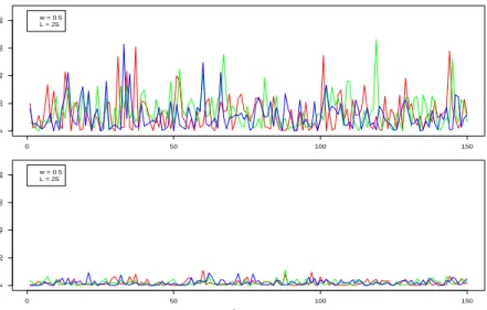
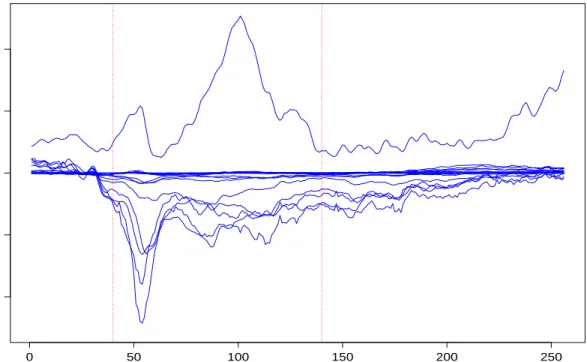
Time 0 50 100 150 0 20 40 60 80 w = 0.5L = 25 Time 0 50 100 150 0 20 40 60 80 w = 0.5L = 25 Time |beta|

Figure 2: |βˆ| for the model with L = 25, τ = 150 and w = 0.5. The panel on the top shows three parameters whose true values are non-zero and the bottom panel shows three parameters whose true values are zero.

is lower, the number of covariates in the overall dataset is huge. For example, with the

Wcut thresholding method in moderate mean complexity case, our model chooses 15

locations for each time point, when the number of locations is considered asL= 50 and

the number of time points is considered as τ = 50. Here, although the original number

of locations for each local model is 50, we are essentially able to achieve lower prediction

error even when the overall number of covariates (L×τ = 2500) is much larger than the

number of observations (n = 100). From Table 2, we see that Wcut thresholding method

can do efficient variable selection compared to Zcut by choosing appropriate number of

locations across time points. We note that within a choice of L, the prediction error

decreases as the number of time points increases. This is an important aspect as EEG

(53)

of the number of locations selected when the algorithm is repeated multiple times.

Figure 2 shows the estimated values of (six locations) parameters ˆβlt. In Figure 2,

the top panel shows the estimated value ˆβlt of three coefficients whose true values are

nonzero across all the time points and the bottom panel shows ˆβlt for those locations

whose true values are zero. These plots show that the algorithm can clearly distinguish

between zero and nonzero coefficients during estimation. Figure 3 shows the

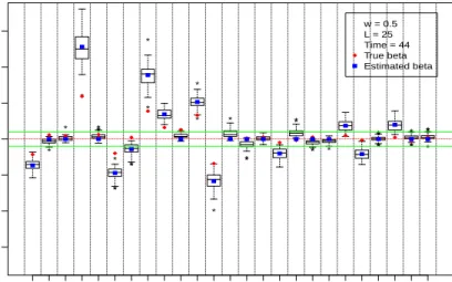
side-by-side boxplots for the MCMC samples ofβ₂ along with their true and estimated values.

Figures 2 and 3 were created under the setting where L= 25, τ = 150, andw= 0.5.

* * * ** *** ** * ** * * * * * * * ** ** ** * * * * * ** * * *** * * **** 1 2 3 4 5 6 7 8 9 11 13 15 17 19 21 23 25 −30 −20 −10 0 10 20 30 w = 0.5 L = 25 Time = 44 True beta Estimated beta Covariates P ar ameter Estimates

Figure 3: MCMC samples of the β₂ (L= 25, τ = 150, and w= 0.5)

2.8