Expected Value and Variance

Chapter 6

Expected Value and Variance

6.1

Expected Value of Discrete Random Variables

When a large collection of numbers is assembled, as in a census, we are usually interested not in the individual numbers, but rather in certain descriptive quantities such as the average or the median. In general, the same is true for the probability distribution of a numerically-valued random variable. In this and in the next section, we shall discuss two such descriptive quantities: theexpected valueand thevariance.

Both of these quantities apply only to numerically-valued random variables, and so we assume, in these sections, that all random variables have numerical values. To give some intuitive justification for our definition, we consider the following game.

Average Value

A die is rolled. If an odd number turns up, we win an amount equal to this number; if an even number turns up, we lose an amount equal to this number. For example, if a two turns up we lose 2, and if a three comes up we win 3. We want to decide if this is a reasonable game to play. We first try simulation. The programDiecarries out this simulation.

The program prints the frequency and the relative frequency with which each outcome occurs. It also calculates the average winnings. We have run the program twice. The results are shown in Table 6.1.

In the first run we have played the game 100 times. In this run our average gain is−.57. It looks as if the game is unfavorable, and we wonder how unfavorable it really is. To get a better idea, we have played the game 10,000 times. In this case our average gain is−.4949.

We note that the relative frequency of each of the six possible outcomes is quite close to the probability 1/6 for this outcome. This corresponds to our frequency interpretation of probability. It also suggests that for very large numbers of plays, our average gain should be

µ = 11 6 −21 6 + 31 6 −41 6 + 51 6 −61 6 225

n = 100 n = 10000

Winning Frequency Relative Frequency Relative

Frequency Frequency 1 17 .17 1681 .1681 -2 17 .17 1678 .1678 3 16 .16 1626 .1626 -4 18 .18 1696 .1696 5 16 .16 1686 .1686 -6 16 .16 1633 .1633

Table 6.1: Frequencies for dice game.

= 9 6 − 12 6 =− 3 6 =−.5.

This agrees quite well with our average gain for 10,000 plays.

We note that the value we have chosen for the average gain is obtained by taking the possible outcomes, multiplying by the probability, and adding the results. This suggests the following definition for the expected outcome of an experiment.

Expected Value

Definition 6.1 LetX be a numerically-valued discrete random variable with sam-ple space Ω and distribution function m(x). The expected value E(X) is defined by

E(X) =X x∈Ω

xm(x),

provided this sum converges absolutely. We often refer to the expected value as the mean, and denote E(X) byµ for short. If the above sum does not converge absolutely, then we say thatX does not have an expected value. 2

Example 6.1 Let an experiment consist of tossing a fair coin three times. Let X denote the number of heads which appear. Then the possible values of X are 0,1,2 and 3. The corresponding probabilities are 1/8,3/8,3/8,and 1/8. Thus, the expected value ofX equals

0 ₁ 8 + 1 ₃ 8 + 2 ₃ 8 + 3 ₁ 8 =3 2 .

Later in this section we shall see a quicker way to compute this expected value, based on the fact thatX can be written as a sum of simpler random variables. 2

Example 6.2 Suppose that we toss a fair coin until a head first comes up, and let X represent the number of tosses which were made. Then the possible values ofX are 1,2, . . ., and the distribution function ofX is defined by

m(i) = 1 2i .

(This is just the geometric distribution with parameter 1/2.) Thus, we have E(X) = ∞ X i=1 i1 2i = ∞ X i=1 1 2i + ∞ X i=2 1 2i +· · · = 1 +1 2 + 1 22 +· · · = 2. 2 Example 6.3 (Example 6.2 continued) Suppose that we flip a coin until a head first appears, and if the number of tosses equals n, then we are paid 2n dollars. What is the expected value of the payment?

We let Y represent the payment. Then, P(Y = 2n) = 1 2n , forn≥1. Thus, E(Y) = ∞ X n=1 2n 1 2n ,

which is a divergent sum. Thus, Y has no expectation. This example is called theSt. Petersburg Paradox. The fact that the above sum is infinite suggests that a player should be willing to pay any fixed amount per game for the privilege of playing this game. The reader is asked to consider how much he or she would be willing to pay for this privilege. It is unlikely that the reader’s answer is more than 10 dollars; therein lies the paradox.

In the early history of probability, various mathematicians gave ways to resolve this paradox. One idea (due to G. Cramer) consists of assuming that the amount of money in the world is finite. He thus assumes that there is some fixed value of nsuch that if the number of tosses equals or exceedsn, the payment is 2n _dollars. The reader is asked to show in Exercise 20 that the expected value of the payment is now finite.

Daniel Bernoulli and Cramer also considered another way to assign value to the payment. Their idea was that the value of a payment is some function of the payment; such a function is now called a utility function. Examples of reasonable utility functions might include the square-root function or the logarithm function. In both cases, the value of 2n dollars is less than twice the value ofn dollars. It can easily be shown that in both cases, the expected utility of the payment is finite

Example 6.4 LetT be the time for the first success in a Bernoulli trials process. Then we take as sample space Ω the integers 1, 2, . . . and assign the geometric distribution m(j) =P(T =j) =qj−1p . Thus, E(T) = 1·p+ 2qp+ 3q2p+· · · = p(1 + 2q+ 3q2+· · ·). Now if|x|<1, then 1 +x+x2+x3+· · ·= 1 1−x . Differentiating this formula, we get

1 + 2x+ 3x2+· · ·= 1 (1−x)2 , so E(T) = p (1−q)2 = p p2 = 1 p .

In particular, we see that if we toss a fair coin a sequence of times, the expected time until the first heads is 1/(1/2) = 2. If we roll a die a sequence of times, the expected number of rolls until the first six is 1/(1/6) = 6. 2

Interpretation of Expected Value

In statistics, one is frequently concerned with the average value of a set of data. The following example shows that the ideas of average value and expected value are very closely related.

Example 6.5 The heights, in inches, of the women on the Swarthmore basketball team are 5’ 9”, 5’ 9”, 5’ 6”, 5’ 8”, 5’ 11”, 5’ 5”, 5’ 7”, 5’ 6”, 5’ 6”, 5’ 7”, 5’ 10”, and 6’ 0”.

A statistician would compute the average height (in inches) as follows: 69 + 69 + 66 + 68 + 71 + 65 + 67 + 66 + 66 + 67 + 70 + 72

12 = 67.9 .

One can also interpret this number as the expected value of a random variable. To see this, let an experiment consist of choosing one of the women at random, and let X denote her height. Then the expected value ofX equals 67.9. 2 Of course, just as with the frequency interpretation of probability, to interpret expected value as an average outcome requires further justification. We know that for any finite experiment the average of the outcomes is not predictable. However, we shall eventually prove that the average will usually be close toE(X) if we repeat the experiment a large number of times. We first need to develop some properties of the expected value. Using these properties, and those of the concept of the variance

X Y HHH 1 HHT 2 HTH 3 HTT 2 THH 2 THT 3 TTH 2 TTT 1

Table 6.2: Tossing a coin three times.

to be introduced in the next section, we shall be able to prove the Law of Large Numbers. This theorem will justify mathematically both our frequency concept of probability and the interpretation of expected value as the average value to be expected in a large number of experiments.

Expectation of a Function of a Random Variable

Suppose that X is a discrete random variable with sample space Ω, and φ(x) is a real-valued function with domain Ω. Then φ(X) is a real-valued random vari-able. One way to determine the expected value ofφ(X) is to first determine the distribution function of this random variable, and then use the definition of expec-tation. However, there is a better way to compute the expected value ofφ(X), as demonstrated in the next example.

Example 6.6 Suppose a coin is tossed 9 times, with the result HHHT T T T HT .

The first set of three heads is called a run. There are three more runs in this sequence, namely the next four tails, the next head, and the next tail. We do not consider the first two tosses to constitute a run, since the third toss has the same value as the first two.

Now suppose an experiment consists of tossing a fair coin three times. Find the expected number of runs. It will be helpful to think of two random variables, X andY, associated with this experiment. We letXdenote the sequence of heads and tails that results when the experiment is performed, andY denote the number of runs in the outcome X. The possible outcomes ofX and the corresponding values ofY are shown in Table 6.2.

To calculate E(Y) using the definition of expectation, we first must find the distribution function m(y) of Y i.e., we group together those values of X with a common value ofY and add their probabilities. In this case, we calculate that the distribution function ofY is: m(1) = 1/4, m(2) = 1/2,andm(3) = 1/4. One easily finds thatE(Y) = 2.

Now suppose we didn’t group the values of X with a common Y-value, but instead, for eachX-valuex, we multiply the probability ofxand the corresponding value ofY, and add the results. We obtain

1 ₁ 8 + 2 ₁ 8 + 3 ₁ 8 + 2 ₁ 8 + 2 ₁ 8 + 3 ₁ 8 + 2 ₁ 8 + 1 ₁ 8 , which equals 2.

This illustrates the following general principle. If X and Y are two random variables, and Y can be written as a function of X, then one can compute the

expected value ofY using the distribution function ofX. 2

Theorem 6.1 If X is a discrete random variable with sample space Ω and distri-bution functionm(x), and ifφ: Ω→R is a function, then

E(φ(X)) =X x∈Ω

φ(x)m(x),

provided the series converges absolutely. 2

The proof of this theorem is straightforward, involving nothing more than group-ing values ofX with a commonY-value, as in Example 6.6.

The Sum of Two Random Variables

Many important results in probability theory concern sums of random variables. We first consider what it means to add two random variables.

Example 6.7 We flip a coin and letX have the value 1 if the coin comes up heads and 0 if the coin comes up tails. Then, we roll a die and letY denote the face that comes up. What does X+Y mean, and what is its distribution? This question is easily answered in this case, by considering, as we did in Chapter 4, the joint random variableZ = (X, Y), whose outcomes are ordered pairs of the form (x, y), where 0 ≤ x ≤ 1 and 1 ≤ y ≤ 6. The description of the experiment makes it reasonable to assume that X and Y are independent, so the distribution function ofZ is uniform, with 1/12 assigned to each outcome. Now it is an easy matter to find the set of outcomes ofX+Y, and its distribution function. 2 In Example 6.1, the random variable X denoted the number of heads which occur when a fair coin is tossed three times. It is natural to think of X as the sum of the random variablesX1, X2, X3, whereXi is defined to be 1 if theith toss comes up heads, and 0 if the ith toss comes up tails. The expected values of the Xi’s are extremely easy to compute. It turns out that the expected value ofX can be obtained by simply adding the expected values of the Xi’s. This fact is stated in the following theorem.

Theorem 6.2 LetX andY be random variables with finite expected values. Then E(X+Y) =E(X) +E(Y),

and ifcis any constant, then

E(cX) =cE(X).

Proof.Let the sample spaces ofX andY be denoted by ΩX and ΩY, and suppose that

ΩX={x1, x2, . . .} and

ΩY ={y1, y2, . . .} .

Then we can consider the random variableX+Y to be the result of applying the functionφ(x, y) =x+yto the joint random variable (X, Y). Then, by Theorem 6.1, we have E(X+Y) = X j X k (xj+yk)P(X =xj, Y =yk) = X j X k xjP(X =xj, Y =yk) +X j X k ykP(X =xj, Y =yk) = X j xjP(X =xj) + X k ykP(Y =yk).

The last equality follows from the fact that

X k P(X =xj, Y =yk) = P(X=xj) and X j P(X =xj, Y =yk) = P(Y =yk). Thus, E(X+Y) =E(X) +E(Y). Ifcis any constant, E(cX) = X j cxjP(X=xj) = cX j xjP(X =xj) = cE(X). 2

X Y a b c 3 a c b 1 b a c 1 b c a 0 c a b 0 c b a 1

Table 6.3: Number of fixed points.

It is easy to prove by mathematical induction that the expected value of the sum of any finite number of random variables is the sum of the expected values of the individual random variables.

It is important to note that mutual independence of the summands was not needed as a hypothesis in the Theorem 6.2 and its generalization. The fact that expectations add, whether or not the summands are mutually independent, is some-times referred to as the First Fundamental Mystery of Probability.

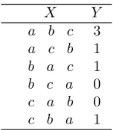
Example 6.8 Let Y be the number of fixed points in a random permutation of the set{a, b, c}. To find the expected value ofY, it is helpful to consider the basic random variable associated with this experiment, namely the random variable X which represents the random permutation. There are six possible outcomes ofX, and we assign to each of them the probability 1/6 see Table 6.3. Then we can calculateE(Y) using Theorem 6.1, as

31 6 + 11 6 + 11 6 + 01 6 + 01 6 + 11 6 = 1.

We now give a very quick way to calculate the average number of fixed points in a random permutation of the set {1,2,3, . . . , n}. Let Z denote the random permutation. For eachi, 1≤i≤n, letXi equal 1 ifZ fixesi, and 0 otherwise. So if we letF denote the number of fixed points inZ, then

F =X1+X2+· · ·+Xn . Therefore, Theorem 6.2 implies that

E(F) =E(X1) +E(X2) +· · ·+E(Xn). But it is easy to see that for eachi,

E(Xi) = 1 n , so

E(F) = 1.

This method of calculation of the expected value is frequently very useful. It applies whenever the random variable in question can be written as a sum of simpler random variables. We emphasize again that it is not necessary that the summands be

Bernoulli Trials

Theorem 6.3 Let Sn be the number of successes in nBernoulli trials with prob-ability pfor success on each trial. Then the expected number of successes is np. That is,

E(Sn) =np .

Proof.LetXj be a random variable which has the value 1 if thejth outcome is a success and 0 if it is a failure. Then, for eachXj,

E(Xj) = 0·(1−p) + 1·p=p . Since

Sn=X1+X2+· · ·+Xn ,

and the expected value of the sum is the sum of the expected values, we have E(Sn) = E(X1) +E(X2) +· · ·+E(Xn)

= np .

2

Poisson Distribution

Recall that the Poisson distribution with parameter λ was obtained as a limit of binomial distributions with parametersnandp, where it was assumed thatnp=λ, andn→ ∞. Since for eachn, the corresponding binomial distribution has expected valueλ, it is reasonable to guess that the expected value of a Poisson distribution with parameterλalso has expectation equal toλ. This is in fact the case, and the reader is invited to show this (see Exercise 21).

Independence

If X and Y are two random variables, it is not true in general that E(X·Y) = E(X)E(Y). However, this is true ifX andY areindependent.

Theorem 6.4 IfX andY are independent random variables, then E(X·Y) =E(X)E(Y).

Proof.Suppose that

ΩX={x1, x2, . . .} and

are the sample spaces ofX andY, respectively. Using Theorem 6.1, we have E(X·Y) =X j X k xjykP(X=xj, Y =yk).

But if X andY are independent,

P(X=xj, Y =yk) =P(X=xj)P(Y =yk). Thus, E(X·Y) = X j X k xjykP(X =xj)P(Y =yk) =   X j xjP(X =xj)   X k ykP(Y =yk) ! = E(X)E(Y). 2 Example 6.9 A coin is tossed twice. Xi = 1 if theith toss is heads and 0 otherwise. We know that X1 and X2 are independent. They each have expected value 1/2. ThusE(X1·X2) =E(X1)E(X2) = (1/2)(1/2) = 1/4. 2 We next give a simple example to show that the expected values need not mul-tiply if the random variables are not independent.

Example 6.10 Consider a single toss of a coin. We define the random variableX to be 1 if heads turns up and 0 if tails turns up, and we set Y = 1−X. Then E(X) = E(Y) = 1/2. But X·Y = 0 for either outcome. Hence, E(X·Y) = 06=

E(X)E(Y). 2

We return to our records example of Section 3.1 for another application of the result that the expected value of the sum of random variables is the sum of the expected values of the individual random variables.

Records

Example 6.11 We start keeping snowfall records this year and want to find the expected number of records that will occur in the next n years. The first year is necessarily a record. The second year will be a record if the snowfall in the second year is greater than that in the first year. By symmetry, this probability is 1/2. More generally, let Xj be 1 if the jth year is a record and 0 otherwise. To find E(Xj), we need only find the probability that the jth year is a record. But the record snowfall for the firstj years is equally likely to fall in any one of these years,

so E(Xj) = 1/j. Therefore, if Sn is the total number of records observed in the firstnyears, E(Sn) = 1 +1 2 + 1 3 +· · ·+ 1 n .

This is the famousdivergent harmonic series. It is easy to show that E(Sn)∼logn

asn→ ∞. A more accurate approximation toE(Sn) is given by the expression logn+γ+ 1

2n ,

whereγ denotes Euler’s constant, and is approximately equal to .5772.

Therefore, in ten years the expected number of records is approximately 2.9298; the exact value is the sum of the first ten terms of the harmonic series which is

2.9290. 2

Craps

Example 6.12 In the game of craps, the player makes a bet and rolls a pair of dice. If the sum of the numbers is 7 or 11 the player wins, if it is 2, 3, or 12 the player loses. If any other number results, sayr, thenrbecomes the player’s point and he continues to roll until eitherror 7 occurs. Ifr comes up first he wins, and if 7 comes up first he loses. The program Craps simulates playing this game a number of times.

We have run the program for 1000 plays in which the player bets 1 dollar each time. The player’s average winnings were −.006. The game of craps would seem to be only slightly unfavorable. Let us calculate the expected winnings on a single play and see if this is the case. We construct a two-stage tree measure as shown in Figure 6.1.

The first stage represents the possible sums for his first roll. The second stage represents the possible outcomes for the game if it has not ended on the first roll. In this stage we are representing the possible outcomes of a sequence of rolls required to determine the final outcome. The branch probabilities for the first stage are computed in the usual way assuming all 36 possibilites for outcomes for the pair of dice are equally likely. For the second stage we assume that the game will eventually end, and we compute the conditional probabilities for obtaining either the point or a 7. For example, assume that the player’s point is 6. Then the game will end when one of the eleven pairs, (1,5), (2,4), (3,3), (4,2), (5,1), (1,6), (2,5), (3,4), (4,3), (5,2), (6,1), occurs. We assume that each of these possible pairs has the same probability. Then the player wins in the first five cases and loses in the last six. Thus the probability of winning is 5/11 and the probability of losing is 6/11. From the path probabilities, we can find the probability that the player wins 1 dollar; it is 244/495. The probability of losing is then 251/495. Thus ifX is his winning for

W L W L W L W L W L W L (2,3,12) L 10 9 8 6 5 4 (7,11) W 1/3 2/3 2/5 3/5 5/11 6/11 5/11 6/11 2/5 3/5 1/3 2/3 2/9 1/12 1/9 5/36 5/36 1/9 1/12 1/9 1/36 2/36 2/45 3/45 25/396 30/396 25/396 30/396 2/45 3/45 1/36 2/36

a dollar bet, E(X) = 1244 495 + (−1)251 495 = − 7 495 ≈ −.0141.

The game is unfavorable, but only slightly. The player’s expected gain innplays is −n(.0141). Ifnis not large, this is a small expected loss for the player. The casino makes a large number of plays and so can afford a small average gain per play and

still expect a large profit. 2

Roulette

Example 6.13 In Las Vegas, a roulette wheel has 38 slots numbered 0, 00, 1, 2, . . . , 36. The 0 and 00 slots are green, and half of the remaining 36 slots are red and half are black. A croupier spins the wheel and throws an ivory ball. If you bet 1 dollar on red, you win 1 dollar if the ball stops in a red slot, and otherwise you lose a dollar. We wish to calculate the expected value of your winnings, if you bet 1 dollar on red.

LetX be the random variable which denotes your winnings in a 1 dollar bet on red in Las Vegas roulette. Then the distribution ofX is given by

mX =

_{−1 1}

20/38 18/38

, and one can easily calculate (see Exercise 5) that

E(X)≈ −.0526.

We now consider the roulette game in Monte Carlo, and follow the treatment of Sagan.1 _{In the roulette game in Monte Carlo there is only one 0. If you bet 1} franc on red and a 0 turns up, then, depending upon the casino, one or more of the following options may be offered:

(a) You get 1/2 of your bet back, and the casino gets the other half of your bet. (b) Your bet is put “in prison,” which we will denote by P1. If red comes up on the next turn, you get your bet back (but you don’t win any money). If black or 0 comes up, you lose your bet.

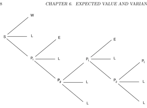
(c) Your bet is put in prisonP1, as before. If red comes up on the next turn, you get your bet back, and if black comes up on the next turn, then you lose your bet. If a 0 comes up on the next turn, then your bet is put into double prison, which we will denote byP2. If your bet is in double prison, and if red comes up on the next turn, then your bet is moved back to prison P1 and the game proceeds as before. If your bet is in double prison, and if black or 0 come up on the next turn, then you lose your bet. We refer the reader to Figure 6.2, where a tree for this option is shown. In this figure,S is the starting position,W means that you win your bet, Lmeans that you lose your bet, andE means that you break even.

S W L E L L L L L L E P_{1 P1} P₁ P₂ P₂ P₂

Figure 6.2: Tree for 2-prison Monte Carlo roulette.

It is interesting to compare the expected winnings of a 1 franc bet on red, under each of these three options. We leave the first two calculations as an exercise (see Exercise 37). Suppose that you choose to play alternative (c). The calculation for this case illustrates the way that the early French probabilists worked problems like this.

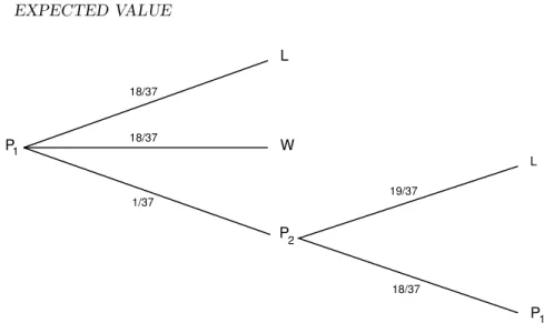
Suppose you bet on red, you choose alternative (c), and a 0 comes up. Your possible future outcomes are shown in the tree diagram in Figure 6.3. Assume that your money is in the first prison and let x be the probability that you lose your franc. From the tree diagram we see that

x= 18 37+

1

37P(you lose your franc|your franc is inP2). Also,

P(you lose your franc|your franc is in P2) =19 37+ 18 37x . So, we have x= 18 37+ 1 37 19 37+ 18 37x .

Solving for x, we obtain x= 685/1351. Thus, starting at S, the probability that you lose your bet equals

18 37+ 1 37x= 25003 49987 .

To find the probability that you win when you bet on red, note that you can only win if red comes up on the first turn, and this happens with probability 18/37. Thus your expected winnings are

1·18 37−1· 25003 49987 =− 687 49987 ≈ −.0137.

P W L P P L 18/37 18/37 1/37 19/37 18/37 1 1 2

Figure 6.3: Your money is put in prison.

It is interesting to note that the more romantic option (c) is less favorable than option (a) (see Exercise 37).

If you bet 1 dollar on the number 17, then the distribution function for your winningsX is PX= −1 35 36/37 1/37 , and the expected winnings are

−1· 36 37+ 35· 1 37 =− 1 37 ≈ −.027.

Thus, at Monte Carlo different bets have different expected values. In Las Vegas almost all bets have the same expected value of −2/38 =−.0526 (see Exercises 4

and 5). 2

Conditional Expectation

Definition 6.2 IfF is any event and X is a random variable with sample space Ω ={x1, x2, . . .}, then theconditional expectation givenF is defined by

E(X|F) =X j

xjP(X =xj|F).

Conditional expectation is used most often in the form provided by the following

theorem. 2

Theorem 6.5 LetXbe a random variable with sample space Ω. IfF1,F2, . . . ,Fr are events such thatFi∩Fj =∅ fori6=j and Ω =∪jFj, then

E(X) =X j

Proof.We have X j E(X|Fj)P(Fj) = X j X k xkP(X =xk|Fj)P(Fj) = X j X k xkP(X =xk andFj occurs) = X k X j xkP(X =xk andFj occurs) = X k xkP(X =xk) = E(X). 2 Example 6.14 (Example 6.12 continued) LetT be the number of rolls in a single play of craps. We can think of a single play as a two-stage process. The first stage consists of a single roll of a pair of dice. The play is over if this roll is a 2, 3, 7, 11, or 12. Otherwise, the player’s point is established, and the second stage begins. This second stage consists of a sequence of rolls which ends when either the player’s point or a 7 is rolled. We record the outcomes of this two-stage experiment using the random variablesX and S, where X denotes the first roll, andS denotes the number of rolls in the second stage of the experiment (of course, S is sometimes equal to 0). Note thatT =S+ 1. Then by Theorem 6.5

E(T) = 12 X j=2 E(T|X =j)P(X=j). If j = 7, 11 or 2, 3, 12, then E(T|X = j) = 1. If j = 4,5,6,8,9, or 10, we can use Example 6.4 to calculate the expected value of S. In each of these cases, we continue rolling until we get either aj or a 7. Thus, S is geometrically distributed with parameter p, which depends upon j. Ifj = 4, for example, the value of pis 3/36 + 6/36 = 1/4. Thus, in this case, the expected number of additional rolls is 1/p= 4, soE(T|X = 4) = 1 + 4 = 5. Carrying out the corresponding calculations for the other possible values ofj and using Theorem 6.5 gives

E(T) = 112 36 +1 + 36 3 + 6 3 36 +1 + 36 4 + 6 4 36 +1 + 36 5 + 6 5 36 +1 + 36 5 + 6 5 36 +1 + 36 4 + 6 4 36 +1 + 36 3 + 6 3 36 = 557 165 ≈ 3.375. . . . 2

Martingales

We can extend the notion of fairness to a player playing a sequence of games by using the concept of conditional expectation.

Example 6.15 LetS1,S2, . . . ,Snbe Peter’s accumulated fortune in playing heads or tails (see Example 1.4). Then

E(Sn|Sn−1=a, . . . , S1=r) = 1

2(a+ 1) + 1

2(a−1) =a .

We note that Peter’s expected fortune after the next play is equal to his present fortune. When this occurs, we say the game is fair. A fair game is also called a

martingale. If the coin is biased and comes up heads with probability pand tails with probabilityq= 1−p, then

E(Sn|Sn−1=a, . . . , S1=r) =p(a+ 1) +q(a−1) =a+p−q .

Thus, ifp < q, this game is unfavorable, and ifp > q, it is favorable. 2 If you are in a casino, you will see players adopting elaborate systems of play to try to make unfavorable games favorable. Two such systems, the martingale doubling system and the more conservative Labouchere system, were described in Exercises 1.1.9 and 1.1.10. Unfortunately, such systems cannot change even a fair game into a favorable game.

Even so, it is a favorite pastime of many people to develop systems of play for gambling games and for other games such as the stock market. We close this section with a simple illustration of such a system.

Stock Prices

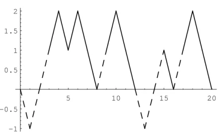
Example 6.16 Let us assume that a stock increases or decreases in value each day by 1 dollar, each with probability 1/2. Then we can identify this simplified model with our familiar game of heads or tails. We assume that a buyer, Mr. Ace, adopts the following strategy. He buys the stock on the first day at its price V. He then waits until the price of the stock increases by one to V + 1 and sells. He then continues to watch the stock until its price falls back toV. He buys again and waits until it goes up toV+ 1 and sells. Thus he holds the stock in intervals during which it increases by 1 dollar. In each such interval, he makes a profit of 1 dollar. However, we assume that he can do this only for a finite number of trading days. Thus he can lose if, in the last interval that he holds the stock, it does not get back up to V + 1; and this is the only way he can lose. In Figure 6.4 we illustrate a typical history if Mr. Ace must stop in twenty days. Mr. Ace holds the stock under his system during the days indicated by broken lines. We note that for the history shown in Figure 6.4, his system nets him a gain of 4 dollars.

We have written a program StockSystemto simulate the fortune of Mr. Ace if he uses his sytem over ann-day period. If one runs this program a large number

5 10 15 20 -1 -0.5 0.5 1 1.5 2

Figure 6.4: Mr. Ace’s system.

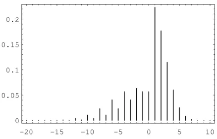
of times, forn= 20, say, one finds that his expected winnings are very close to 0, but the probability that he is ahead after 20 days is significantly greater than 1/2. For small values of n, the exact distribution of winnings can be calculated. The distribution for the case n = 20 is shown in Figure 6.5. Using this distribution, it is easy to calculate that the expected value of his winnings is exactly 0. This is another instance of the fact that a fair game (a martingale) remains fair under quite general systems of play.

Although the expected value of his winnings is 0, the probability that Mr. Ace is ahead after 20 days is about .610. Thus, he would be able to tell his friends that his system gives him a better chance of being ahead than that of someone who simply buys the stock and holds it, if our simple random model is correct. There have been a number of studies to determine how random the stock market is. 2

Historical Remarks

With the Law of Large Numbers to bolster the frequency interpretation of proba-bility, we find it natural to justify the definition of expected value in terms of the average outcome over a large number of repetitions of the experiment. The concept of expected value was used before it was formally defined; and when it was used, it was considered not as an average value but rather as the appropriate value for a gamble. For example recall, from the Historical Remarks section of Chapter 1, Section 1.2, Pascal’s way of finding the value of a three-game series that had to be called off before it is finished.

Pascal first observed that if each player has only one game to win, then the stake of 64 pistoles should be divided evenly. Then he considered the case where one player has won two games and the other one.

Then consider, Sir, if the first man wins, he gets 64 pistoles, if he loses he gets 32. Thus if they do not wish to risk this last game, but wish

-20 -15 -10 -5 0 5 10 0 0.05 0.1 0.15 0.2

Figure 6.5: Winnings distribution forn= 20.

to separate without playing it, the first man must say: “I am certain to get 32 pistoles, even if I lose I still get them; but as for the other 32 pistoles, perhaps I will get them, perhaps you will get them, the chances are equal. Let us then divide these 32 pistoles in half and give one half to me as well as my 32 which are mine for sure.” He will then have 48 pistoles and the other 16.2

Note that Pascal reduced the problem to a symmetric bet in which each player gets the same amount and takes it as obvious that in this case the stakes should be divided equally.

The first systematic study of expected value appears in Huygens’ book. Like Pascal, Huygens find the value of a gamble by assuming that the answer is obvious for certain symmetric situations and uses this to deduce the expected for the general situation. He does this in steps. His first proposition is

Prop. I. If I expect aor b, either of which, with equal probability, may fall to me, then my Expectation is worth (a+b)/2, that is, the half Sum ofaandb.3

Huygens proved this as follows: Assume that two player A and B play a game in which each player puts up a stake of (a+b)/2 with an equal chance of winning the total stake. Then the value of the game to each player is (a+b)/2. For example, if the game had to be called off clearly each player should just get back his original stake. Now, by symmetry, this value is not changed if we add the condition that the winner of the game has to pay the loser an amount b as a consolation prize. Then for player A the value is still (a+b)/2. But what are his possible outcomes

2_{Quoted in F. N. David,Games, Gods and Gambling(London: Griffin, 1962), p. 231.} 3_{C. Huygens,Calculating in Games of Chance,translation attributed to John Arbuthnot} (Lon-don, 1692), p. 34.

for the modified game? If he wins he gets the total stakea+band must pay B an amount b so ends up witha. If he loses he gets an amount bfrom player B. Thus player A winsaorbwith equal chances and the value to him is (a+b)/2.

Huygens illustrated this proof in terms of an example. If you are offered a game in which you have an equal chance of winning 2 or 8, the expected value is 5, since this game is equivalent to the game in which each player stakes 5 and agrees to pay the loser 3 — a game in which the value is obviously 5.

Huygens’ second proposition is

Prop. II. If I expect a,b, orc, either of which, with equal facility, may happen, then the Value of my Expectation is (a+b+c)/3, or the third of the Sum ofa,b, andc.4

His argument here is similar. Three players, A, B, and C, each stake (a+b+c)/3

in a game they have an equal chance of winning. The value of this game to player A is clearly the amount he has staked. Further, this value is not changed if A enters into an agreement with B that if one of them wins he pays the other a consolation prize ofband with C that if one of them wins he pays the other a consolation prize ofc. By symmetry these agreements do not change the value of the game. In this modified game, if A wins he wins the total stakea+b+c minus the consolation prizes b+c giving him a final winning ofa. If B wins, A wins b and if C wins, A winsc. Thus A finds himself in a game with value (a+b+c)/3 and with outcomes a,b, and coccurring with equal chance. This proves Proposition II.

More generally, this reasoning shows that if there arenoutcomes a1, a2, . . . , an ,

all occurring with the same probability, the expected value is a1+a2+· · ·+an

n .

In his third proposition Huygens considered the case where you winaor b but with unequal probabilities. He assumed there are pchances of winning a, and q chances of winning b, all having the same probability. He then showed that the expected value is

E= p

p+q ·a+ q p+q·b .

This follows by considering an equivalent gamble withp+qoutcomes all occurring with the same probability and with a payoff ofainpof the outcomes andbinqof the outcomes. This allowed Huygens to compute the expected value for experiments with unequal probabilities, at least when these probablities are rational numbers.

Thus, instead of defining the expected value as a weighted average, Huygens assumed that the expected value of certain symmetric gambles are known and de-duced the other values from these. Although this requires a good deal of clever

manipulation, Huygens ended up with values that agree with those given by our modern definition of expected value. One advantage of this method is that it gives a justification for the expected value in cases where it is not reasonable to assume that you can repeat the experiment a large number of times, as for example, in betting that at least two presidents died on the same day of the year. (In fact, three did; all were signers of the Declaration of Independence, and all three died on July 4.)

In his book, Huygens calculated the expected value of games using techniques similar to those which we used in computing the expected value for roulette at Monte Carlo. For example, his proposition XIV is:

Prop. XIV. If I were playing with another by turns, with two Dice, on this Condition, that if I throw 7 I gain, and if he throws 6 he gains allowing him the first Throw: To find the proportion of my Hazard to his.5

A modern description of this game is as follows. Huygens and his opponent take turns rolling a die. The game is over if Huygens rolls a 7 or his opponent rolls a 6. His opponent rolls first. What is the probability that Huygens wins the game?

To solve this problem Huygens letxbe his chance of winning when his opponent threw first andy his chance of winning when he threw first. Then on the first roll his opponent wins on 5 out of the 36 possibilities. Thus,

x= 31 36·y .

But when Huygens rolls he wins on 6 out of the 36 possible outcomes, and in the other 30, he is led back to where his chances arex. Thus

y= 6 36+

30 36·x .

From these two equations Huygens found thatx= 31/61.

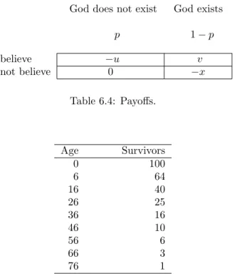
Another early use of expected value appeared in Pascal’s argument to show that a rational person should believe in the existence of God.6 _{Pascal said that we have} to make a wager whether to believe or not to believe. Letpdenote the probability that God does not exist. His discussion suggests that we are playing a game with two strategies, believe and not believe, with payoffs as shown in Table 6.4.

Here −u represents the cost to you of passing up some worldly pleasures as a consequence of believing that God exists. If you do not believe, and God is a vengeful God, you will lose x. If God exists and you do believe you will gain v. Now to determine which strategy is best you should compare the two expected values

p(−u) + (1−p)v and p0 + (1−p)(−x), 5_{ibid., p. 47.}

6_{Quoted in I. Hacking, The Emergence of Probability (Cambridge: Cambridge Univ. Press,} 1975).

God does not exist God exists p 1−p believe −u v not believe 0 −x Table 6.4: Payoffs. Age Survivors 0 100 6 64 16 40 26 25 36 16 46 10 56 6 66 3 76 1

Table 6.5: Graunt’s mortality data.

and choose the larger of the two. In general, the choice will depend upon the value of p. But Pascal assumed that the value ofvis infinite and so the strategy of believing is best no matter what probability you assign for the existence of God. This example is considered by some to be the beginning of decision theory. Decision analyses of this kind appear today in many fields, and, in particular, are an important part of medical diagnostics and corporate business decisions.

Another early use of expected value was to decide the price of annuities. The study of statistics has its origins in the use of the bills of mortality kept in the parishes in London from 1603. These records kept a weekly tally of christenings and burials. From these John Graunt made estimates for the population of London and also provided the first mortality data,7 _{shown in Table 6.5.}

As Hacking observes, Graunt apparently constructed this table by assuming that after the age of 6 there is a constant probability of about 5/8 of surviving for another decade.8 _{For example, of the 64 people who survive to age 6, 5/8 of} 64 or 40 survive to 16, 5/8 of these 40 or 25 survive to 26, and so forth. Of course, he rounded off his figures to the nearest whole person.

Clearly, a constant mortality rate cannot be correct throughout the whole range, and later tables provided by Halley were more realistic in this respect.9

7_{ibid., p. 108.} 8_{ibid., p. 109.}

Aterminal annuity provides a fixed amount of money during a period ofnyears. To determine the price of a terminal annuity one needs only to know the appropriate interest rate. Alife annuityprovides a fixed amount during each year of the buyer’s life. The appropriate price for a life annuity is the expected value of the terminal annuity evaluated for the random lifetime of the buyer. Thus, the work of Huygens in introducing expected value and the work of Graunt and Halley in determining mortality tables led to a more rational method for pricing annuities. This was one of the first serious uses of probability theory outside the gambling houses.

Although expected value plays a role now in every branch of science, it retains its importance in the casino. In 1962, Edward Thorp’s book Beat the Dealer10

provided the reader with a strategy for playing the popular casino game of blackjack that would assure the player a positive expected winning. This book forevermore changed the belief of the casinos that they could not be beat.

Exercises

1 A card is drawn at random from a deck consisting of cards numbered 2 through 10. A player wins 1 dollar if the number on the card is odd and loses 1 dollar if the number if even. What is the expected value of his win-nings?

2 A card is drawn at random from a deck of playing cards. If it is red, the player wins 1 dollar; if it is black, the player loses 2 dollars. Find the expected value of the game.

3 In a class there are 20 students: 3 are 5’ 6”, 5 are 5’8”, 4 are 5’10”, 4 are 6’, and 4 are 6’ 2”. A student is chosen at random. What is the student’s expected height?

4 In Las Vegas the roulette wheel has a 0 and a 00 and then the numbers 1 to 36 marked on equal slots; the wheel is spun and a ball stops randomly in one slot. When a player bets 1 dollar on a number, he receives 36 dollars if the ball stops on this number, for a net gain of 35 dollars; otherwise, he loses his dollar bet. Find the expected value for his winnings.

5 In a second version of roulette in Las Vegas, a player bets on red or black. Half of the numbers from 1 to 36 are red, and half are black. If a player bets a dollar on black, and if the ball stops on a black number, he gets his dollar back and another dollar. If the ball stops on a red number or on 0 or 00 he loses his dollar. Find the expected winnings for this bet.

6 A die is rolled twice. LetX denote the sum of the two numbers that turn up, andY the difference of the numbers (specifically, the number on the first roll minus the number on the second). Show that E(XY) =E(X)E(Y). AreX andY independent?

vol. 17 (1693), pp. 596–610; 654–656.

*7 Show that, ifX andY are random variables taking on only two values each, and ifE(XY) =E(X)E(Y), thenX andY are independent.

8 A royal family has children until it has a boy or until it has three children, whichever comes first. Assume that each child is a boy with probability 1/2. Find the expected number of boys in this royal family and the expected num-ber of girls.

9 If the first roll in a game of craps is neither a natural nor craps, the player can make an additional bet, equal to his original one, that he will make his point before a seven turns up. If his point is four or ten he is paid off at 2 : 1 odds; if it is a five or nine he is paid off at odds 3 : 2; and if it is a six or eight he is paid off at odds 6 : 5. Find the player’s expected winnings if he makes this additional bet when he has the opportunity.

10 In Example 6.16 assume that Mr. Ace decides to buy the stock and hold it until it goes up 1 dollar and then sell and not buy again. Modify the program

StockSystem to find the distribution of his profit under this system after a twenty-day period. Find the expected profit and the probability that he comes out ahead.

11 On September 26, 1980, the New York Times reported that a mysterious stranger strode into a Las Vegas casino, placed a single bet of 777,000 dollars on the “don’t pass” line at the crap table, and walked away with more than 1.5 million dollars. In the “don’t pass” bet, the bettor is essentially betting with the house. An exception occurs if the roller rolls a 12 on the first roll. In this case, the roller loses and the “don’t pass” better just gets back the money bet instead of winning. Show that the “don’t pass” bettor has a more favorable bet than the roller.

12 Recall that in themartingale doubling system(see Exercise 1.1.10), the player doubles his bet each time he loses. Suppose that you are playing roulette in a fair casinowhere there are no 0’s, and you bet on red each time. You then win with probability 1/2 each time. Assume that you enter the casino with 100 dollars, start with a 1-dollar bet and employ the martingale system. You stop as soon as you have won one bet, or in the unlikely event that black turns up six times in a row so that you are down 63 dollars and cannot make the required 64-dollar bet. Find your expected winnings under this system of play.

13 You have 80 dollars and play the following game. An urn contains two white balls and two black balls. You draw the balls out one at a time without replacement until all the balls are gone. On each draw, you bet half of your present fortune that you will draw a white ball. What is your expected final fortune?

14 In the hat check problem (see Example 3.12), it was assumed thatN people check their hats and the hats are handed back at random. LetXj = 1 if the

jth person gets his or her hat and 0 otherwise. Find E(Xj) and E(Xj·Xk) forj not equal tok. AreXj andXk independent?

15 A box contains two gold balls and three silver balls. You are allowed to choose successively balls from the box at random. You win 1 dollar each time you draw a gold ball and lose 1 dollar each time you draw a silver ball. After a draw, the ball is not replaced. Show that, if you draw until you are ahead by 1 dollar or until there are no more gold balls, this is a favorable game.

16 Gerolamo Cardano in his book, The Gambling Scholar, written in the early 1500s, considers the following carnival game. There are six dice. Each of the dice has five blank sides. The sixth side has a number between 1 and 6—a different number on each die. The six dice are rolled and the player wins a prize depending on the total of the numbers which turn up.

(a) Find, as Cardano did, the expected total without finding its distribution. (b) Large prizes were given for large totals with a modest fee to play the

game. Explain why this could be done.

17 LetXbe the first time that afailureoccurs in an infinite sequence of Bernoulli trials with probability pfor success. Let pk =P(X =k) fork = 1, 2, . . . . Show that pk =pk−1_{q where q = 1−p. Show that} P

kpk = 1. Show that E(X) = 1/q. What is the expected number of tosses of a coin required to obtain the first tail?

18 Exactly one of six similar keys opens a certain door. If you try the keys, one after another, what is the expected number of keys that you will have to try before success?

19 A multiple choice exam is given. A problem has four possible answers, and exactly one answer is correct. The student is allowed to choose a subset of the four possible answers as his answer. If his chosen subset contains the correct answer, the student receives three points, but he loses one point for each wrong answer in his chosen subset. Show that if he just guesses a subset uniformly and randomly his expected score is zero.

20 You are offered the following game to play: a fair coin is tossed until heads turns up for the first time (see Example 6.3). If this occurs on the first toss you receive 2 dollars, if it occurs on the second toss you receive 22_{= 4 dollars} and, in general, if heads turns up for the first time on thenth toss you receive 2n _dollars.

(a) Show that the expected value of your winnings does not exist (i.e., is given by a divergent sum) for this game. Does this mean that this game is favorable no matter how much you pay to play it?

(b) Assume that you only receive 210 dollars if any number greater than or equal to ten tosses are required to obtain the first head. Show that your expected value for this modified game is finite and find its value.

(c) Assume that you pay 10 dollars for each play of the original game. Write a program to simulate 100 plays of the game and see how you do. (d) Now assume that the utility ofndollars is √n. Write an expression for

the expected utility of the payment, and show that this expression has a finite value. Estimate this value. Repeat this exercise for the case that the utility function is log(n).

21 Let X be a random variable which is Poisson distributed with parameterλ. Show thatE(X) =λ. Hint: Recall that

ex= 1 +x+x 2 2! +

x3 3! +· · ·.

22 Recall that in Exercise 1.1.14, we considered a town with two hospitals. In the large hospital about 45 babies are born each day, and in the smaller hospital about 15 babies are born each day. We were interested in guessing which hospital would have on the average the largest number of days with the property that more than 60 percent of the children born on that day are boys. For each hospital find the expected number of days in a year that have the property that more than 60 percent of the children born on that day were boys.

23 An insurance company has 1,000 policies on men of age 50. The company estimates that the probability that a man of age 50 dies within a year is .01. Estimate the number of claims that the company can expect from beneficiaries of these men within a year.

24 Using the life table for 1981 in Appendix C, write a program to compute the expected lifetime for males and females of each possible age from 1 to 85. Compare the results for males and females. Comment on whether life insur-ance should be priced differently for males and females.

*25 A deck of ESP cards consists of 20 cards each of two types: say ten stars, ten circles (normally there are five types). The deck is shuffled and the cards turned up one at a time. You, the alleged percipient, are to name the symbol on each cardbefore it is turned up.

Suppose that you are really just guessing at the cards. If you do not get to see each card after you have made your guess, then it is easy to calculate the expected number of correct guesses, namely ten.

If, on the other hand, you are guessing with information, that is, if you see each card after your guess, then, of course, you might expect to get a higher score. This is indeed the case, but calculating the correct expectation is no longer easy.

But it is easy to do a computer simulation of this guessing with information, so we can get a good idea of the expectation by simulation. (This is similar to the way that skilled blackjack players make blackjack into a favorable game by observing the cards that have already been played. See Exercise 29.)

(a) First, do a simulation of guessing without information, repeating the experiment at least 1000 times. Estimate the expected number of correct answers and compare your result with the theoretical expectation. (b) What is the best strategy for guessing with information?

(c) Do a simulation of guessing with information, using the strategy in (b). Repeat the experiment at least 1000 times, and estimate the expectation in this case.

(d) LetSbe the number of stars andCthe number of circles in the deck. Let h(S, C) be the expected winnings using the optimal guessing strategy in (b). Show thath(S, C) satisfies the recursion relation

h(S, C) = S S+Ch(S−1, C) + C S+Ch(S, C−1) + max(S, C) S+C , and h(0,0) = h(−1,0) = h(0,−1) = 0. Using this relation, write a program to computeh(S, C) and findh(10,10). Compare the computed value of h(10,10) with the result of your simulation in (c). For more about this exercise and Exercise 26 see Diaconis and Graham.11

*26 Consider the ESP problem as described in Exercise 25. You are again guessing with information, and you are using the optimal guessing strategy of guessing

star if the remaining deck has more stars,circleif more circles, and tossing a coin if the number of stars and circles are equal. Assume thatS ≥C, where S is the number of stars and Cthe number of circles.

We can plot the results of a typical game on a graph, where the horizontal axis represents the number of steps and the vertical axis represents the difference

between the number of stars and the number of circles that have been turned up. A typical game is shown in Figure 6.6. In this particular game, the order in which the cards were turned up is (C, S, S, S, S, C, C, S, S, C). Thus, in this particular game, there were six stars and four circles in the deck. This means, in particular, that every game played with this deck would have a graph which ends at the point (10,2). We define the lineLto be the horizontal line which goes through the ending point on the graph (so its vertical coordinate is just the difference between the number of stars and circles in the deck).

(a) Show that, when the random walk is below the lineL, the player guesses right when the graph goes up (star is turned up) and, when the walk is above the line, the player guesses right when the walk goes down (circle turned up). Show from this property that the subject is sure to have at leastS correct guesses.

(b) When the walk is at a point (x, x)onthe lineLthe number of stars and circles remaining is the same, and so the subject tosses a coin. Show that 11_{P. Diaconis and R. Graham, “The Analysis of Sequential Experiments with Feedback to} Sub-jects,”Annals of Statistics,vol. 9 (1981), pp. 3–23.

2

1

1 2 3 4 5 6 7 8 9 10

(10,2) L

Figure 6.6: Random walk for ESP.

the probability that the walk reaches (x, x) is S x C x S+C 2x .

Hint: The outcomes of 2x cards is a hypergeometric distribution (see Section 5.1).

(c) Using the results of (a) and (b) show that the expected number of correct guesses under intelligent guessing is

S+ C X x=1 1 2 S x C x S+C 2x .

27 It has been said12 _{that a Dr. B. Muriel Bristol declined a cup of tea stating} that she preferred a cup into which milk had been poured first. The famous statistician R. A. Fisher carried out a test to see if she could tell whether milk was put in before or after the tea. Assume that for the test Dr. Bristol was given eight cups of tea—four in which the milk was put in before the tea and four in which the milk was put in after the tea.

(a) What is the expected number of correct guesses the lady would make if she had no information after each test and was just guessing?

(b) Using the result of Exercise 26 find the expected number of correct guesses if she was told the result of each guess and used an optimal guessing strategy.

28 In a popular computer game the computer picks an integer from 1 to n at random. The player is givenkchances to guess the number. After each guess the computer responds “correct,” “too small,” or “too big.”

(a) Show that ifn≤2k−1, then there is a strategy that guarantees you will correctly guess the number inktries.

(b) Show that ifn≥2k−1, there is a strategy that assures you of identifying one of 2k _{−1 numbers and hence gives a probability of (2}k _{−1)/n of} winning. Why is this an optimal strategy? Illustrate your result in terms of the casen= 9 and k= 3.

29 In the casino game of blackjack the dealer is dealt two cards, one face up and one face down, and each player is dealt two cards, both face down. If the dealer is showing an ace the player can look at his down cards and then make a bet called an insurance bet. (Expert players will recognize why it is called insurance.) If you make this bet you will win the bet if the dealer’s second card is a ten card: namely, a ten, jack, queen, or king. If you win, you are paid twice your insurance bet; otherwise you lose this bet. Show that, if the only cards you can see are the dealer’s ace and your two cards and if your cards are not ten cards, then the insurance bet is an unfavorable bet. Show, however, that if you are playing two hands simultaneously, and you have no ten cards, then it is a favorable bet. (Thorp13 _{has shown that the game of} blackjack is favorable to the player if he or she can keep good enough track of the cards that have been played.)

30 Assume that, every time you buy a box of Wheaties, you receive a picture of one of the nplayers for the New York Yankees (see Exercise 3.2.34). LetXk be the number of additional boxes you have to buy, after you have obtained k−1 different pictures, in order to obtain the next new picture. ThusX1= 1, X2is the number of boxes bought after this to obtain a picture different from the first pictured obtained, and so forth.

(a) Show thatXk has a geometric distribution withp= (n−k+ 1)/n. (b) Simulate the experiment for a team with 26 players (25 would be more

accurate but we want an even number). Carry out a number of simula-tions and estimate the expected time required to get the first 13 players and the expected time to get the second 13. How do these expectations compare?

(c) Show that, if there are 2nplayers, the expected time to get the first half of the players is 2n ₁ 2n+ 1 2n−1 +· · ·+ 1 n+ 1 , and the expected time to get the second half is

2n ₁ n+ 1 n−1 +· · ·+ 1 . 13_{E. Thorp,Beat the Dealer(New York: Random House, 1962).}

(d) In Example 6.11 we stated that 1 +1 2 + 1 3 +· · ·+ 1 n ∼logn+.5772 + 1 2n .

Use this to estimate the expression in (c). Compare these estimates with the exact values and also with your estimates obtained by simulation for the case n= 26.

*31 (Feller14) A large number, N, of people are subjected to a blood test. This can be administered in two ways: (1) Each person can be tested separately, in this case N test are required, (2) the blood samples of k persons can be pooled and analyzed together. If this test is negative, this one test suffices for the kpeople. If the test is positive,each of thek persons must be tested separately, and in all,k+ 1 tests are required for the kpeople. Assume that the probability p that a test is positive is the same for all people and that these events are independent.

(a) Find the probability that the test for a pooled sample of k people will be positive.

(b) What is the expected value of the number X of tests necessary under plan (2)? (Assume thatN is divisible by k.)

(c) For smallp, show that the value of kwhich will minimize the expected number of tests under the second plan is approximately 1/√p.

32 Write a program to add random numbers chosen from [0,1] until the first time the sum is greater than one. Have your program repeat this experiment a number of times to estimate the expected number of selections necessary in order that the sum of the chosen numbers first exceeds 1. On the basis of your experiments, what is your estimate for this number?

*33 The following related discrete problem also gives a good clue for the answer to Exercise 32. Randomly select with replacementt1,t2, . . . ,trfrom the set (1/n,2/n, . . . , n/n). Let X be the smallest value ofrsatisfying

t1+t2+· · ·+tr>1.

Then E(X) = (1 + 1/n)n. To prove this, we can just as well choose t1, t2, . . . ,trrandomly with replacement from the set (1,2, . . . , n) and letX be the smallest value ofr for which

t1+t2+· · ·+tr> n . (a) Use Exercise 3.2.36 to show that

P(X ≥j+ 1) = _n j 1 n j .

14_{W. Feller,Introduction to Probability Theory and Its Applications,3rd ed., vol. 1 (New York:} John Wiley and Sons, 1968), p. 240.

(b) Show that E(X) = n X j=0 P(X ≥j+ 1).

(c) From these two facts, find an expression forE(X). This proof is due to Harris Schultz.15

*34 (Banach’s Matchbox16_{) A man carries in each of his two front pockets a box} of matches originally containing N matches. Whenever he needs a match, he chooses a pocket at random and removes one from that box. One day he reaches into a pocket and finds the box empty.

(a) Letprdenote the probability that the other pocket contains rmatches. Define a sequence ofcounter random variables as follows: Let Xi = 1 if theith draw is from the left pocket, and 0 if it is from the right pocket. Interpret pr in terms of Sn = X1+X2+· · ·+Xn. Find a binomial expression forpr.

(b) Write a computer program to compute thepr, as well as the probability that the other pocket contains at least r matches, for N = 100 and r from 0 to 50.

(c) Show that (N−r)pr= (1/2)(2N+ 1)pr+1−(1/2)(r+ 1)pr+1 . (d) EvaluateP

rpr.

(e) Use (c) and (d) to determine the expectationE of the distribution{pr}. (f) Use Stirling’s formula to obtain an approximation for E. How many matches must each box contain to ensure a value of about 13 for the expectationE? (Takeπ= 22/7.)

35 A coin is tossed until the first time a head turns up. If this occurs on thenth toss and nis odd you win 2n_{/n, but ifnis even then you lose 2}n_{/n. Then if} your expected winnings exist they are given by the convergent series

1−1 2+ 1 3 − 1 4 +· · ·

called the alternatingharmonic series. It is tempting to say that this should be the expected value of the experiment. Show that if we were to do this, the expected value of an experiment would depend upon the order in which the outcomes are listed.

36 Suppose we have an urn containingcyellow balls anddgreen balls. We draw k balls, without replacement, from the urn. Find the expected number of yellow balls drawn. Hint: Write the number of yellow balls drawn as the sum ofc random variables.

15_{H. Schultz, “An Expected Value Problem,” Two-Year Mathematics Journal,vol. 10, no. 4} (1979), pp. 277–78.

37 The reader is referred to Example 6.13 for an explanation of the various op-tions available in Monte Carlo roulette.

(a) Compute the expected winnings of a 1 franc bet on red under option (a). (b) Repeat part (a) for option (b).

(c) Compare the expected winnings for all three options.

*38 (from Pittel17_{) Telephone books, n in number, are kept in a stack. The} probability that the book numbered i (where 1≤ i ≤n) is consulted for a given phone call is pi > 0, where the pi’s sum to 1. After a book is used, it is placed at the top of the stack. Assume that the calls are independent and evenly spaced, and that the system has been employed indefinitely far into the past. Let di be the average depth of book iin the stack. Show that di ≤ dj whenever pi ≥ pj. Thus, on the average, the more popular books have a tendency to be closer to the top of the stack. Hint: Letpij denote the probability that bookiis above book j. Show thatpij=pij(1−pj) +pjipi.

*39 (from Propp18_{) In the previous problem, let P be the probability that at the} present time, each book is in its proper place, i.e., bookiisith from the top. Find a formula for P in terms of the pi’s. In addition, find the least upper bound on P, if thepi’s are allowed to vary. Hint: First find the probability that book 1 is in the right place. Then find the probability that book 2 is in the right place, given that book 1 is in the right place. Continue.

*40 (from H. Shultz and B. Leonard19_{) A sequence of random numbers in [0,1)} is generated until the sequence is no longer monotone increasing. The num-bers are chosen according to the uniform distribution. What is the expected length of the sequence? (In calculating the length, the term that destroys monotonicity is included.) Hint: Let a1, a2, . . .be the sequence and let X denote the length of the sequence. Then

P(X > k) =P(a1< a2<· · ·< ak),

and the probability on the right-hand side is easy to calculate. Furthermore, one can show that

E(X) = 1 +P(X >1) +P(X >2) +· · · .

41 Let T be the random variable that counts the number of 2-unshuffles per-formed on ann-card deck until all of the labels on the cards are distinct. This random variable was discussed in Section 3.3. Using Equation 3.4 in that section, together with the formula

E(T) =

∞

X

s=0

P(T > s)

17_{B. Pittel, Problem #1195,Mathematics Magazine,vol. 58, no. 3 (May 1985), pg. 183.} 18_{J. Propp, Problem #1159,Mathematics Magazinevol. 57, no. 1 (Feb. 1984), pg. 50.} 19_{H. Shultz and B. Leonard, “Unexpected Occurrences of the Numbere,”Mathematics Magazine} vol. 62, no. 4 (October, 1989), pp. 269-271.

that was proved in Exercise 33, show that E(T) = ∞ X s=0 1− ₂s n _n! 2sn .

Show that forn= 52, this expression is approximately equal to 11.7. (As was stated in Chapter 3, this means that on the average, almost 12 riffle shuffles of a 52-card deck are required in order for the process to be considered random.)

6.2

Variance of Discrete Random Variables

The usefulness of the expected value as a prediction for the outcome of an ex-periment is increased when the outcome is not likely to deviate too much from the expected value. In this section we shall introduce a measure of this deviation, called the variance.

Variance

Definition 6.3 LetXbe a numerically valued random variable with expected value µ=E(X). Then the variance ofX, denoted byV(X), is

V(X) =E((X−µ)2).

2

Note that, by Theorem 6.1,V(X) is given by V(X) =X

x

(x−µ)2m(x), (6.1)

wheremis the distribution function ofX.

Standard Deviation

The standard deviation of X, denoted by D(X), is D(X) = pV(X). We often writeσforD(X) andσ2 _forV(X).

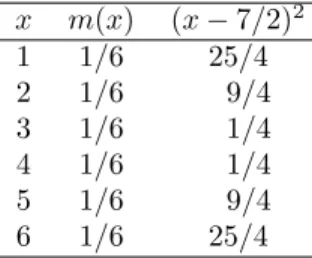
Example 6.17 Consider one roll of a die. LetX be the number that turns up. To findV(X), we must first find the expected value of X. This is

µ = E(X) = 11 6 + 21 6 + 31 6 + 41 6 + 51 6 + 61 6 = 7 2 .

To find the variance of X, we form the new random variable (X −µ)2 _and compute its expectation. We can easily do this using the following table.

x m(x) (x−7/2)2 1 1/6 25/4 2 1/6 9/4 3 1/6 1/4 4 1/6 1/4 5 1/6 9/4 6 1/6 25/4

Table 6.6: Variance calculation.

From this table we findE((X−µ)2_{) is} V(X) = 1 6 ₂₅ 4 + 9 4 + 1 4 + 1 4+ 9 4 + 25 4 = 35 12 ,

and the standard deviationD(X) =p35/12≈1.707. 2

Calculation of Variance

We next prove a theorem that gives us a useful alternative form for computing the variance.

Theorem 6.6 IfX is any random variable withE(X) =µ, then V(X) =E(X2)−µ2 .

Proof.We have

V(X) = E((X−µ)2) =E(X2−2µX+µ2) = E(X2)−2µE(X) +µ2=E(X2)−µ2.

2

Using Theorem 6.6, we can compute the variance of the outcome of a roll of a die by first computing

E(X2) = 11 6 + 41 6 + 91 6 + 161 6 + 251 6 + 361 6 = 91 6 , and, V(X) =E(X2)−µ2=91 6 − 7 2 2 = 35 12 ,

Properties of Variance

The variance has properties very different from those of the expectation. Ifcis any constant,E(cX) =cE(X) andE(X+c) =E(X) +c. These two statements imply that the expectation is a linear function. However, the variance is not linear, as seen in the next theorem.

Theorem 6.7 IfX is any random variable andc is any constant, then V(cX) =c2V(X)

and

V(X+c) =V(X).

Proof.Letµ=E(X). ThenE(cX) =cµ, and

V(cX) = E((cX−cµ)2) =E(c2(X−µ)2) = c2E((X−µ)2) =c2V(X).

To prove the second assertion, we note that, to compute V(X+c), we would replacexbyx+candµbyµ+cin Equation 6.1. Then thec’s would cancel, leaving

V(X). 2

We turn now to some general properties of the variance. Recall that ifXandY are any two random variables,E(X+Y) =E(X)+E(Y). This is not always true for the case of the variance. For example, letX be a random variable withV(X)6= 0, and define Y =−X. Then V(X) =V(Y), so that V(X) +V(Y) = 2V(X). But X+Y is always 0 and hence has variance 0. ThusV(X+Y)6=V(X) +V(Y).

In the important case of mutually independent random variables, however, the variance of the sum is the sum of the variances.

Theorem 6.8 LetX andY be twoindependent random variables. Then V(X+Y) =V(X) +V(Y).

Proof.LetE(X) =aandE(Y) =b. Then V(X+Y) = E((X+Y)2)−(a+b)2

= E(X2) + 2E(XY) +E(Y2)−a2−2ab−b2 . SinceX andY are independent,E(XY) =E(X)E(Y) =ab. Thus,

V(X+Y) =E(X2)−a2+E(Y2)−b2=V(X) +V(Y).

It is easy to extend this proof, by mathematical induction, to show that the variance of the sum of any number of mutually independent random variables is the sum of the individual variances. Thus we have the following theorem.

Theorem 6.9 LetX1,X2, . . . ,Xnbe an independent trials process withE(Xj) = µandV(Xj) =σ2. Let

Sn=X1+X2+· · ·+Xn be the sum, and

An= Sn n be the average. Then

E(Sn) = nµ , V(Sn) = nσ2 , σ(Sn) = σ√n , E(An) = µ , V(An) = σ 2 n , σ(An) = σ √ n .

Proof.Since all the random variables Xj have the same expected value, we have

E(Sn) =E(X1) +· · ·+E(Xn) =nµ , V(Sn) =V(X1) +· · ·+V(Xn) =nσ2 , and

σ(Sn) =σ√n .

We have seen that, if we multiply a random variableXwith meanµand variance σ2 _{by a constant c, the new random variable has expected value cµ and variance} c2_σ2_{. Thus,} E(An) =E _Sn n = nµ n =µ , and V(An) =V _Sn n =V(Sn) n2 = nσ2 n2 = σ2 n . Finally, the standard deviation ofAn is given by

σ(An) = √σ n .

1 2 3 4 5 6 0 0.1 0.2 0.3 0.4 0.5 0.6 2 2.5 3 3.5 4 4.5 5 0 0.5 1 1.5 2 n = 10 n = 100

Figure 6.7: Empirical distribution ofAn.

The last equation in the above theorem implies that in an independent trials process, if the individual summands have finite variance, then the standard devi-ation of the average goes to 0 as n → ∞. Since the standard deviation tells us something about the spread of the distribution around the mean, we see that for large values of n, the value ofAn is usually very close to the mean of An, which equals µ, as shown above. This statement is made precise in Chapter 8, where it is called the Law of Large Numbers. For example, letX represent the roll of a fair die. In Figure 6.7, we show the distribution of a random variableAn corresponding toX, forn= 10 andn= 100.

Example 6.18 Considernrolls of a die. We have seen that, if Xj is the outcome if thejth roll, thenE(Xj) = 7/2 andV(Xj) = 35/12. Thus, ifSn is the sum of the outcomes, andAn=Sn/nis the average of the outcomes, we haveE(An) = 7/2 and V(An) = (35/12)/n. Therefore, as n increases, the expected value of the average remains constant, but the variance tends to 0. If the variance is a measure of the expected deviation from the mean this would indicate that, for large n, we can expect the average to be very near the expected value. This is in fact the case, and

we shall justify it in Chapter 8. 2

Bernoulli Trials

Consider next the general Bernoulli trials process. As usual, we letXj = 1 if the jth outcome is a success and 0 if it is a failure. Ifpis the probability of a success, andq= 1−p, then E(Xj) = 0q+ 1p=p , E(X_j2) = 02q+ 12p=p , and V(Xj) =E(Xj2)−(E(Xj)) 2 =p−p2=pq .

Thus, for Bernoulli trials, ifSn=X1+X2+· · ·+Xnis the number of successes, thenE(Sn) =np,V(Sn) =npq, andD(Sn) =√npq.If An =Sn/n is the average number of successes, then E(An) =p, V(An) =pq/n, andD(An) =ppq/n. We see that the expected proportion of successes remainspand the variance tends to 0.

This suggests that the frequency interpretation of probability is a correct one. We shall make this more precise in Chapter 8.

Example 6.19 Let T denote the number of trials until the first success in a Bernoulli trials process. Then T is geometrically distributed. What is the vari-ance ofT? In Example 4.15, we saw that

mT =

_{1 2 3 · · ·}

p qp q2p · · ·

. In Example 6.4, we showed that

E(T) = 1/p . Thus,

V(T) =E(T2)−1/p2 , so we need only find

E(T2) = 1p+ 4qp+ 9q2p+· · · = p(1 + 4q+ 9q2+· · ·). To evaluate this sum, we start again with

1 +x+x2+· · ·= 1 1−x . Differentiating, we obtain 1 + 2x+ 3x2+· · ·= 1 (1−x)2 . Multiplying byx, x+ 2x2+ 3x3+· · ·= x (1−x)2 . Differentiating again gives

1 + 4x+ 9x2+· · ·= 1 +x (1−x)3 . Thus, E(T2) =p 1 +q (1−q)3 = 1 +q p2 and V(T) = E(T2)−(E(T))2 = 1 +q p2 − 1 p2 = q p2 .

For example, the variance for the number of tosses of a coin until the first head turns up is (1/2)/(1/2)2 _{= 2. The variance for the number of rolls of a} die until the first six turns up is (5/6)/(1/6)2= 30. Note that, aspdecreases, the variance increases rapidly. This corresponds to the increased spread of the geometric