Inferring differences between
networks using Bayesian exponential
random graph models
Application to brain functional connectivity
Brieuc Charles Louis Lehmann
MRC Biostatistics Unit University of Cambridge
This dissertation is submitted for the degree of Doctor of Philosophy
Declaration
This thesis is the result of my own work and includes nothing which is the outcome of work done in collaboration except as declared in the Preface and specified in the text. It is not substantially the same as any that I have submitted, or, is being concurrently submitted for a degree or diploma or other qualification at the University of Cambridge or any other University or similar institution except as declared in the Preface and specified in the text. I further state that no substantial part of my thesis has already been submitted, or, is being concurrently submitted for any such degree, diploma or other qualification at the University of Cambridge or any other University or similar institution except as declared in the Preface and specified in the text. It does not exceed the prescribed word limit for the relevant Degree Committee.
Inferring differences between networks using
Bayesian exponential random graph models
Application to brain functional connectivity
Brieuc Charles Louis Lehmann
The goal of many neuroimaging studies is to better understand how the functional con-nectivity structure of the brain changes with a given phenotype such as age. Functional connectivity can be characterised as a network, with nodes corresponding to brain regions and edges corresponding to statistical dependencies between the respective regional time series of activity. A typical neuroimaging dataset will thus consist of one or more networks for each individual in the study. Most statistical network models, however, were originally proposed to describe a single underlying relational structure such as friendships between individuals or hyperlinks between web pages. As a result, the development of these mod-els has largely been restricted to the single network case. While one could in principle fit a single network model to each individual separately, it is not always straightforward to combine these individual results into a single group result.
In the first half of the thesis, we propose a multilevel framework for populations of networks based on exponential random graph models. By pooling information across the individual networks, this framework provides a principled approach to characterise the relational structure for an entire population. We use the framework to assess group-level variations in functional connectivity, providing a method for the inference of differences in the topological structure between groups of networks. Our motivation stems from the Cam-CAN project, a neuroimaging study on healthy ageing. Using this dataset, we illus-trate how our method can be used to detect differences in functional connectivity between a group of young individuals and a group of old individuals.
In the second half of the thesis, we shift our focus to dynamic functional connectivity (dFC). Recent studies have found that using static measures may average over informative fluctuations in functional connectivity. Several methods have been developed to measure dFC in functional magnetic resonance imaging (fMRI) data. However, spurious group differences in measured dFC may be caused by other sources of heterogeneity between people. We use a generic simulation framework for fMRI data to investigate the effect of such heterogeneity on estimates of dFC and find that, despite no differences in true dFC, individual differences in measured dFC can result from other (non-dynamic) features of the data. We then add a natural and novel extension to our multilevel framework by inserting time windows as an intermediate level between time points and subjects. Using magnetoencephalography data from the Cam-CAN study, we apply our method to detect differences in time-varying connectivity between a young group and an old group.
Acknowledgements
This thesis would not have been possible without the financial, academic and personal support from a wide range of sources. I am very grateful for funding from the Medical Research Council and the Cambridge Philosophical Society. I am also thankful for travel funds from COSTNET, ISBA, and Trinity College, Cambridge, which permitted me to attend a number of highly rewarding conferences and workshops.
The patience and guidance of my supervisors Simon White, Rik Henson and Linda Geerligs proved invaluable throughout the course of my PhD. The MRC Biostatistics Unit provided a rich environment to explore new ideas; I am especially indebted to Rob Goudie, Fiona Matthews and Stephen Hill for their useful suggestions. I would not be where I am now without the inspiration of my teachers, particularly Vadim Myslov for first sparking my interest in statistics, John Aston for introducing me to statistical neuroimaging, and Ton Coolen for his advice and encouragement.
While progress towards the completion of this thesis was patchy at times, the support from my family and friends was unfailing. I am grateful to Roxana, Mycroft, Micah, Nel-son, Esma, Fabian, Ruth, Sofia, Max, Drakˇso, Wiktor, Maciek, Filip, and Ravi (amongst many others) for all the great times we spent together, and I look forward to sharing many more. Finally, to Paula, thank you for your companionship and unwavering support.
Contents
1 Introduction 1
1.1 Functional connectivity . . . 2
1.2 Networks in neuroimaging . . . 6
1.3 The Cam-CAN study . . . 9
1.4 Outline of thesis . . . 9
2 A multilevel framework for populations of networks using exponential random graph models 11 2.1 Exponential random graph models . . . 12
2.2 Bayesian inference for ERGMs . . . 16
2.3 A framework for populations of networks . . . 19
2.4 Model assessment . . . 27
2.5 Computational efficiency . . . 36
2.6 Future work . . . 55
3 Inferring group-level differences in functional connectivity with Bayesian exponential random graph models 57 3.1 Background . . . 58
3.3 Methods . . . 64
3.4 Results . . . 75
3.5 Discussion . . . 86
4 Assessing dynamic functional connectivity in heterogeneous samples 91 4.1 Background . . . 92
4.2 Methods: simulation framework . . . 95
4.3 Methods: specific simulations . . . 98
4.4 Results . . . 106
4.5 Discussion . . . 129
4.6 Future work . . . 133
5 Modelling dynamic functional connectivity with Bayesian exponential random graph models 135 5.1 Background . . . 136 5.2 Data . . . 137 5.3 Methods . . . 140 5.4 Results . . . 147 5.5 Discussion . . . 155 6 Conclusion 165 6.1 Challenges . . . 165 6.2 Future work . . . 168
Chapter 1
Introduction
The human brain is a vastly complex system that, at multiple spatial scales, can be use-fully characterised as distinct units in interaction with each other [22]. At the smallest scale, the units are neurons while at the other end of the scale, the units are entire brain regions. Recently, there has been a shift in cognitive neuroscience away from a modular approach (focus on units) to a network approach (focus on interactions) [20]. Mount-ing evidence indicates that treatMount-ing brain regions as independent processors is misguided [49]; gaining insight into cognitive function requires an understanding of how distinct brain areas work in conjunction [50].
Different neuroimaging modalities allow researchers to probe different types of brain connectivity: structural, functional, or effective. Structural, or anatomical, connectivity refers to the physical links between distinct brain regions and can be measured, for exam-ple, using diffusion tensor imaging [4]. In contrast, functional and effective connectivity are both based on neural activity. This neural activity can be measured, for example, using functional magnetic resonance imaging (fMRI) [120] or magnetoencephalography (MEG) [21]. Functional connectivity, the focus of this thesis, corresponds to the statisti-cal interdependence of neural activity in different regions. Effective connectivity refers to the influence of brain regions on one another. While functional connectivity is a notion of undirected dependencies, effective connectivity aims to capture the causal effects of neural activity between brain regions.
Network theory provides a natural framework to model brain connectivity. The brain units correspond to the nodes of a network, or graph, and the interactions to the edges between the nodes. Recent developments in network theory [81, 103] have provided a wide range of tools for neuroscientists to study the brain. These have largely consisted
of various network measures that quantify different aspects of the brain’s connectivity structure [121].
The goal of many neuroimaging studies is to better understand how brain connectiv-ity changes with a given phenotype such as age [52], cognitive function [155] or disease status [5, 32]. In the context of network theory, this amounts to a problem of network comparisons. To assess group-level variations in brain connectivity, it is therefore crucial to develop statistical methods for the inference of differences in the topological struc-ture between groups of networks. Given the complex strucstruc-ture of network data, this is a challenging task and the development of such methods is still in its infancy.
In the remainder of this Introduction, we review functional connectivity (Section 1.1), the use of networks in neuroimaging (Section 1.2), and introduce the Cambridge Centre for Ageing and Neuroscience (Cam-CAN) study (Section 1.3).
1.1
Functional connectivity
Neural activity can today be measured using a number of neuroimaging technologies, including functional magnetic resonance imaging (fMRI), and magnetoencephalography (MEG). In the modular approach to neuroscience, a typical neuroimaging study would aim to detect which brain regions are more active when performing a particular task [63]. In contrast, the network approach focuses on functional connectivity, the relationship be-tween the neural activity of distinct brain regions [46]. While this connectivity can also be measured in a task-based experiment, our focus will be on resting-state studies in which subjects are told to relax and not think of anything in particular [153]. To appreciate the implications and limitations of functional connectivity studies, it is crucial to understand how it is measured. In this section, we briefly review the physics and biology behind fMRI and MEG, as well as the different metrics used to characterise functional connectivity.
Functional magnetic resonance imaging
Functional magnetic resonance imaging (fMRI) measures brain activity by detecting changes in blood flow [63]. Neural activity in a given region triggers a haemodynamic response, in which blood flow to the region increases temporarily in order to satisfy the local energy requirement. Importantly, this process results in an increase in the ratio of oxygenated haemoglobin to deoxygenated haemoglobin. The fMRI scanner exploits
the different magnetic properties of oxygenated haemoglobin compared to deoxygenated haemoglobin to localise neural activity at a given point in time.
The scanner generates three-dimensional volumes of the brain over time. Each volume is made up of voxels, cuboids with dimensions usually in the range of 2-4mm. (The voxel is the 3D equivalent of the more commonly-known 2D image unit, the pixel.) In a typical fMRI scan, a normal sized brain consists of roughly 100,000-150,000 voxels. The time taken to generate a single volume, known as the sampling rate or repetition time (TR), typically lies between TR = 1s and TR = 3s.
Given their large number, it is common to cluster voxels together into regions of in-terest (ROIs) [111]. This procedure, known as parcellation, serves to both reduce the dimensionality of the data and improve its interpretability. Many diverse parcellation schemes exist, varying both in the number of ROIs and in how these ROIs are defined [150, 66, 37]. When applied to an fMRI scan, the result of each of these schemes is a representative time series of neural activity for each ROI. Mathematically, this can be described as a multivariate time series {Xt}Tt=1 where T is the number of samples and
each component {Xr t}
T
t=1 corresponds to a ROI r. One can then investigate the brain’s functional connectivity structure by studying the statistical interdependence of these com-ponent time series.
fMRI provides an indirect measure of neural activity (through blood flow) that is susceptible to various sources of noise such as head motion [64], scanner drift [136], and cardiovascular effects [34]. This is particularly troublesome in the context of group studies or heterogeneous samples; different groups or subjects may have differing haemodynamic properties or levels of noise. For example, the shape of the haemodynamic response func-tion (HRF), which describes the blood flow following neural activity, is known to vary with age [73]. While extensive preprocessing pipelines serve to reduce the effects of these confounds, they cannot be mitigated completely. It is important to keep this fact in mind when comparing functional connectivity across groups as differences may arise due to variations in such confounds rather than true differences in the neural co-activation structure.
Magnetoencephalography
Magnetoencephalography (MEG) is another functional neuroimaging technique that mea-sures the magnetic fields induced by neural activity [65]. Modern MEG scanners consist of around 300 sensors that detect the magnetic field at carefully selected locations around
the head. In contrast with fMRI, this provides a more direct measure of neural activity rather than a surrogate such as blood flow. On the other hand, the MEG scanner only provides recordings at the sensor locations, not at the true electrical sources inside the head that generate the magnetic fields outside the head.
The problem of transforming the data from sensor space to source space is known as an inverse problem. The challenge is to reconstruct the electrical activity from regions within the brain (source location) from the magnetic field detected at the sensor locations, where the number of regions is greater than the number of sensors. One popular approach for this is beamforming [157]. Beamforming is a spatial filtering technique that estimates the source activity at locations on a regular three-dimensional grid within the brain. The main assumption underlying beamforming is that the activity at distinct sources is un-correlated. This somewhat limits the spatial resolution of MEG to several millimetres as sources close to each other are likely to exhibit correlated neural activity. As with fMRI, one can then perform a parcellation step to obtain an estimate of neural activity for ROIs from the beamformed data.
The temporal resolution of MEG, however, is typically on the order of milliseconds, making it capable of capturing extremely rapid oscillatory signals of brain activity [13]. Given the higher temporal resolution, it is typical to analyse MEG in different frequency bands: θ (4Hz to 7Hz), α (8Hz to 13Hz), β (13Hz to 30Hz), low γ (30Hz to 50Hz), and high γ (50Hz to 100Hz). Different frequency bands have been found to correspond to different neuronal processes [94].
Connectivity measures
In both the cases of fMRI and MEG, time series of measured neural activity for a number of ROIs are obtained. To analyse the functional connectivity structure of the ROIs re-quires a measure of co-activation between these time series. While there exists a plethora of different functional connectivity metrics [159, 17], each with their own strengths and weaknesses, we focus on Pearson correlation, which can be applied to both the amplitude of fMRI signal and the amplitude envelope of oscillatory activity in different frequency bands for MEG [71].
Pearson correlation is the most common measure of functional connectivity in fMRI [120]. Given two time series {Xr
t} T t=1 and {X s t} T
Pearson correlation between the two ROIs is given by ρr,s= PT t=1(X r t −X¯r)(Xts−X¯s) q PT t=1(X r t −X¯r)2 PT t=1(X s t −X¯s)2 (1.1) where ¯Xr = 1 T PT t=1X r t.
Amplitude envelope correlation measures the Pearson correlation between the loga-rithm of the amplitude envelopes of two signals. LetXr(t) be the continuous-time signal
associated with ROIr. The corresponding analytic signal is given by
hr(t) =Xr(t) +iH[Xr(t)] (1.2)
where H[Xr(t)] is the Hilbert transform of Xr(t). The amplitude envelope of Xr(t) is
given by the magnitude of the analytic signal |hr(t)|. From existing resting-state MEG
functional connectivity metrics, amplitude envelope correlation was found to be the most reliable [31].
Time-varying functional connectivity
The measures described above are typically calculated for the entire duration of the scan. Recent evidence, however, suggests that, even in resting-state, these functional tions change over the course of a scan [7, 26, 80]. Moreover, dynamic functional connec-tivity (dFC) approaches, which measure such changes in connections, have been used to identify biomarkers for schizophrenia [122] and Alzheimer’s disease [78].
The majority of dFC studies apply a sliding-window analysis to the ROI time series. This involves creating w equally spaced (tapered) windows of the same size which cover the length of the time series. For each window, connectivity between ROIs (typically Pearson correlation) is calculated for the windowed time series consisting only of the time points within that window. The windows are typically overlapping and thus able to detect faster fluctuations compared to disjoint windows, at the cost of introducing dependency between connectivity estimates in nearby windows. This yields a time series of length w
consisting of connectivity measures (correlation) for each pair of ROIs.
Methods to analyse the resulting correlation time series range from the relatively sim-ple (e.g. characterising dFC as the standard deviation or power of the correlation time series [42]) to the more sophisticated (e.g. identifying recurring connectivity patterns
using k-means clustering [7]). Most approaches, however, do not account for heterogene-ity between individuals. Heterogeneheterogene-ity can arise in a variety of ways, including vascular differences or degrees of head motion, which may have a range of effects on observed func-tional connectivity dynamics. While the effect of such heterogeneity on static connectivity has been studied previously [95, 11, 114], the impact on dFC measures is less explored.
1.2
Networks in neuroimaging
Network construction
The measures of functional connectivity defined in the previous section quantify pairwise interactions between any two ROIs. The extension to whole-brain functional connectivity is straightforward: compute the pairwise metric between each pair of ROIs. This yields a symmetric connectivity matrix C ∈ RR×R where R is the number of ROIs. The
con-nectivity matrix can be associated with a weighted network with nodes corresponding to each column or row, and edge weights given by the corresponding entries in the matrix. Note that, with probability one, all of the entries inC are non-zero and so the associated network is fully connected. This network, however, is likely to include a significant pro-portion of spurious connections due to, for example, the presence of measurement noise [1].
This problem is addressed by applying a threshold to the connectivity matrix to set all weak or negative connections to zero. To gain insight into the topological properties of the brain’s connectivity structure, it is typical to then binarise the resulting network by setting all remaining non-zero connections to one. Specifically, the binarisation procedure is performed by applying a threshold cthresh to the connectivity matrix C such that a
connection exists between ROIs r and s if and only if Crs ≥cthresh:
Ars = 1 if Crs≥cthresh 0 otherwise. (1.3)
The adjacency matrix A ∈ {0,1}R×R defines a graph: Ars = 1 if an edge (connection)
exists between nodes (ROIs) r and s, and Ars = 0 otherwise. An example of a binarised
functional connectivity network is shown in Figure 1.1.
num-Figure 1.1: An example of a binarised functional connectivity network. This image was created using BrainNet Viewer [164].
ber of choices to be made, each of which will have an impact on the subsequent analysis. First, to reduce the dimensionality of the data, the brain is parcellated into distinct brain regions and a representative time course constructed for each region. The regions define the nodes of the network and different parcellations yield networks of different sizes. Sec-ond, weighted edges are defined via a pairwise functional connectivity metric, typically Pearson correlation, between regional time courses. Thirdly, these edges are thresholded and binarised to yield a sparse, unweighted network. The choice of threshold also has important implications for the resulting network structure [156, 60]. While there are a variety of thresholding schemes, the most common approach is to selectcthresh to yield a
network of a given density, typically between 5% and 50% [44].
There is no single correct way to construct a network from functional brain imaging data; each of the choices outlined above should be motivated by the scientific question at hand. Nevertheless, the framework presented in this thesis is applicable to any set of networks, regardless of how they are constructed.
Network modelling
The application of graph theory to brain connectivity, both structural and functional, has become increasingly popular in recent years [22]. Early graph-theoretical studies focused on comparisons to random networks via the computation of various network metrics. For
example, functional brain networks as measured by both fMRI and MEG were found to have a shorter average path length and a higher clustering coefficient than expected in a random network [2, 139]. Network metrics were then employed to quantify differences be-tween groups of individuals, for example young people versus old people [98] and patients with Alzheimer’s disease versus healthy subjects [141].
This approach suffers from a serious limitation: network metrics are influenced by the overall density of the network [62]. As a result, it is difficult to disentangle differences in more complex topological properties such as clustering from differences in the network density. This is particularly important in the context of ageing since mean functional connectivity is known to decrease with age [54]. Note that it is not trivial to simply con-trol for network density when comparing network metrics due to their highly non-linear relationship.
One possible means to address this issue is to use exponential random graph models (ERGMs). An exponential random graph model is a set of parametric statistical distri-butions on network data (see [118] for a review). The aim of the model is to characterise the distribution of a network in terms of a set of summary statistics, or network metrics. This is especially useful in the context of neuroimaging: a better understanding of how (local) topological features give rise to the brain’s global network structure could yield crucial insights into the processes that underlie cognitive function. Moreover, by including network density along with other metrics of interest in the model, ERGMs provide a way to quantify their relative influence on the overall network structure while accounting for the density.
ERGMs have been applied successfully to characterise both functional connectivity [132, 131, 104] and structural connectivity [134]. To date, there have been two proposed approaches for using ERGMs in group studies. The first approach constructs a single group network by keeping edges that are present in a minimum of the individual net-works, and then fits an ERGM to the group network [134]. The main drawback of this approach lies in the averaging over information present in the individual networks. In contrast, the second approach fits an ERGM to each individual network and then takes the mean or median of the fitted parameters to represent the group-level connectivity structure [131, 104]. While this is preferable to the first approach, taking a simple mean or median seems oversimplistic. The main contribution of this thesis is to develop a mul-tilevel framework for ERGMs, thus allowing information to be pooled across networks and providing a mechanism to infer group-level differences in connectivity structure.
1.3
The Cam-CAN study
The motivating application for this thesis derives from the Cambridge Centre for Ageing and Neuroscience (Cam-CAN) research project [127], which aims to improve understand-ing of the effect of healthy ageunderstand-ing on cognitive and brain function. The Cam-CAN dataset consists of a range of cognitive tests and functional neuroimaging experiments for approx-imately 650 healthy individuals aged 18-87 (roughly 100 per age decade, though with fewer in the youngest decade). Our focus will be on the youngest decade (18-27) and the oldest decade (78-87); the aim will be to compare the functional connectivity structure between these two groups.
1.4
Outline of thesis
The core of the thesis is contained in Chapters 2-5. Chapter 2 introduces the main methodological development: a multilevel framework for populations of networks based on exponential random graph models. Chapter 3 applies this framework to resting-state functional connectivity networks constructed from data from the Cam-CAN study. Using this dataset, we illustrate how our method can be used to detect differences in functional connectivity between a group of young individuals and a group of old individuals. In Chapter 4, we shift our focus to dynamic functional connectivity and develop a generic simulation framework for fMRI data. We then use simulations to investigate the effect of various sources of heterogeneity on estimates of dFC. Chapter 5 extends the multilevel framework for use with time-varying connectivity networks. Using MEG data from the Cam-CAN study, we apply the extended method to detect differences in time-varying connectivity between a young group and an old group. Finally, Chapter 6 discusses some of the challenges and limitations of the work presented in the thesis, and identifies some avenues for future work.
Chapter 2
A multilevel framework for
populations of networks using
exponential random graph models
Summary
Most statistical network models were originally proposed to describe a single underlying relational structure such as friendships between individuals or hyperlinks between web pages. As a result, the development of these models has largely been restricted to the single network case. Most neuroimaging datasets, however, consist of multiple networks across several individuals. For such studies, a typical goal is to infer a common con-nectivity structure across individuals. While one could in principle fit a single network model to each individual separately, it is not always straightforward to combine these individual results into a single group result. Using Bayesian exponential random graph models, we propose a multilevel framework for populations of networks. By pooling in-formation across the individual networks, this framework provides a principled approach to characterise the relational structure for an entire population.
This chapter consists of the following: Section 2.1 presents the exponential random graph model (ERGM); Section 2.2 discusses Bayesian inference for ERGMs; Section 2.3 introduces both the multilevel framework extending the Bayesian ERGM to populations of networks and the model fitting procedure; Section 2.4 outlines how we perform model assessment within the framework; and Section 2.5 describes improvements to the fitting procedure in the name of computational efficiency.
2.1
Exponential random graph models
An exponential random graph model is a set of parametric statistical distributions on network data (see [118] for a review). The aim of the model is to characterise the distri-bution of a network in terms of a set of summary statistics. These summary statistics are typically comprised of topological features of the network, such as the number of edges and subgraph counts. The summary statistics enter the likelihood via a weighted sum; the weights are (unknown) model parameters that quantify the relative influence of the corresponding summary statistic on the overall network structure and must be inferred from the data. ERGMs are thus a flexible way in which to describe the global network structure as a function of network summary statistics.
Notation
We first introduce some notation and terminology. Let G = (V,E) be a random network consisting of afixed setV of nodes and arandom setE of undirected edges. WriteV =|V|
for the (fixed) number of nodes ofG. The sample space ofE is Ω ={0,1}V(V2−1); there can
either be an edge (1) or not an edge (0) between the V(V2−1) pairs of nodes in V. Write
E = |E| for the number of edges in G. Note that E itself is a random variable that can take values between 0 (an empty network) and V(V2−1) (a complete network).
We will exclusively work with the adjacency matrixY associated with the network G. (We will use the term network to refer to both G and Y.) The adjacency matrix Y is a symmetric random matrix taking values in Y = {0,1}V×V. Specifically, Yij = Yji = 1
if there is an edge e ∈ E between nodes i ∈ V and j ∈ V. Denote y to be an instanti-ation, or outcome, of the random adjacency matrix Y and write P(Y = y) := π(y) for the probability that Y takes the value y. Let Y be the range of Y, i.e. the set of all possible outcomes. Lets(Y) denote a vector ofpsummary statistics ofY, such that each component is a function si :Y →R.
We reserve non-italicised boldface type for matrices (such as Y and Σ) and generally use non-boldface type for scalars and vectors.
Summary statistics
In the context of ERGMs, a summary statistic is simply a network metric, i.e. a real-valued function of some configuration of edges in the network. Simple examples include
Summary statistic Description
edges Number of edges
k-cycle Number of k-cycles
k-star Number of k-stars
k-degree Number of nodes with degree k
geometrically weighted degree distribution (GWDEG)
Weighted degree distribution with weight for k -degree given by (1 + exp(−τ))k where τ is a fixed
decay parameter
k dyadwise shared partners Number of node pairs having exactlyk shared part-ners
geometrically weighted dyad-wise shared partner distribution (GWDSP)
Weighted distribution of dyadwise shared partners with weight fork edgewise shared partners given by (1 + exp(−τ))k whereτ is a fixed decay parameter
k edgewise shared partners Number of connected node pairs having exactly k
shared partners geometrically weighted
edge-wise shared partner distribution (GWESP)
Weighted distribution of edgewise shared partners with weight fork edgewise shared partners given by (1 + exp(−τ))k whereτ is a fixed decay parameter
k non-edgewise shared partners Number ofunconnected node pairs having exactly k
shared partners geometrically weighted
non-edgewise shared partner distri-bution (GWNSP)
Weighted distribution of non-edgewise shared part-ners with weight fork non-edgewise shared partners given by (1 + exp(−τ))k where τ is a fixed decay parameter
Table 2.1: A selection of summary statistics commonly used in ERGMs.
the number of edges or triangles. (Some other common choices can be found in Table 2.1.) The summary statistics included in a given ERGM represent those configurations expected to appear more frequently or less frequently than in a random graph. In other words, the choice of summary statistics is a modelling decision; it reflects our belief of how the global network structure may be summarised and is driven by the context of the network. The flexibility of ERGMs derives from the range and number of possible sum-mary statistics that can be used [117]. Note that each distinct set of sumsum-mary statistics (up to rescaling) defines a different ERGM.
Definition
We are now equipped to define an exponential random graph model. Let Y be a net-work, and lets(Y) be a vector-valued function ofpsummary statistics defined onY. The probability mass function of Y under the corresponding ERGM is given by π(y|θ) where
π(y|θ) = exp
θTs(y)
Z(θ) . (2.1)
Here, θ ∈ Θ ⊆ Rp is a vector of p model parameters that must be estimated from the
data and Z(θ) =P
y0∈Yexp
θTs(y0) is the normalising constant ensuring the
probabil-ity mass function sums to one. Given data, that is, an observation yof Y, the goal is to infer which values of θ best correspond to the data under this distribution.
Remarks
Exponential random graph models are a flexible family of distributions on networks that aim to characterise the global network structure in terms of a relatively small number of summary statistics on the network. This is especially useful in the context of neuroimag-ing: a better understanding of how (local) topological features give rise to the brain’s global network structure could yield crucial insights into the processes that underlie cog-nitive function. One particular challenge in network neuroscience arises from the fact that network metrics are influenced by the overall density of the network [62]. In the con-text of ageing, for example, mean functional connectivity is known to decrease with age [54], making it difficult to disentangle differences in more complex topological properties such as clustering from differences in the network density. By including network density along with other metrics of interest in the model, ERGMs provide a way to quantify their relative influence on the overall network structure while accounting for the density.
The flexibility of the family stems from the range and number of summary statistics that can be included in the model. Given a choice of summary statistics, the model parameters θ quantify the relative influence of the corresponding statistic on the overall structure of the network. To see this, consider the log-odds of an edgeYij, conditional on
observing the rest of the network. Denote Ycij =Y\Yij to be the set of variables in the
random adjacency matrix Y excluding that of the random variable Yij associated with
the single node pair (i, j). Denoteyc
ij to be the corresponding observations of Y c
log P(Yij = 1|Ycij =ycij) P(Yij = 0|Ycij =ycij) = log P(Yij = 1,Ycij =ycij) P(Yij = 0,Ycij =ycij) =θT{s(y+ij)−s(y−ij)} (2.2)
where y+ij is the network with Yij = 1 and Ycij = ycij, and similarly y
−
ij is the same
net-work except Yij = 0. Thus, each component of θ can be interpreted as the difference in
conditional log-odds per unit change in the corresponding summary statistic between the networksy+ij and y−ij. All else being equal, a larger value of the θ component places more weight on networksy with a larger value of the corresponding summary statistic.
The main barrier to inference is the normalising constant Z(θ). This is the sum of the numerator over all possible networks in Y and so, even for moderately sized net-works, is typically intractable. For example, a network with just 10 nodes has 210(102−1) =
35,184,372,088,832 possible network configurations. As a result, computing the sum
Z(θ) = P
y0∈Yexp
θTs(y0) over all these configurations is infeasible. We will thus refer
toZ(θ) as anintractable normalising constant, or INC, because we cannot compute it in sensible time.
Although ERGMs are a powerful and flexible class of distributions, they have a num-ber of limitations. For example, ERGMs have been found to suffer from degeneracy issues [137, 67]. This refers to the model estimation problems that result from certain model specifications. Specifically, under such specifications, the model places disproportionate mass on empty or fully connected networks. Since inference methods for ERGMs rely on MCMC simulation from the model, the result is that the chain moves to and stays at an empty or full network, irrespective of the observed network. Degeneracy occurs as a result of model misspecification and may be overcome by using summary statistics that are less prone to degeneracy issues [138]. Another limitation is that ERGM coefficients are not necessarily comparable across networks of different sizes [87]. Thus, our proposed framework is restricted to the case where each of the networks have the same number of nodes. This is not a major problem in the context of a neuroimaging study because the same parcellation is typically applied to each brain scan, resulting in the same number of nodes.
2.2
Bayesian inference for ERGMs
In what follows, we will work in the Bayesian paradigm, treating the model parameters
θ as random variables. The Bayesian formulation of ERGMs was first suggested in [82] and then expanded upon in [24]. Through the machinery of Bayesian hierarchical mod-elling, we shall see that this provides a natural framework for populations of networks, as typically found in neuroimaging datasets.
To fully specify a Bayesian ERGM, we need only augment the definition in (2.1) with a prior distribution π(θ) for the model parameters. Given an observation yof the network, we can then perform inference by analysing the posterior distribution π(θ|y). Through Bayes’ rule, we may write the posterior as
π(θ|y) = π(y|θ)π(θ) π(y) = exp θTs(y) π(θ) Z(θ)π(y) (2.3)
where π(y) = RΘπ(y|θ)π(θ)dθ is the model evidence. The posterior distribution is gen-erally not available in a closed-form expression. This is due to two properties of the posterior: first, the (standard) intractability of the model evidence, and second, the in-tractability of the likelihood via the INC Z(θ). Posterior distributions with these two sources of intractability are referred to as doubly-intractable.
Although the distribution is not available in closed-form, we can nevertheless use nu-merical methods to study the posterior. Our aim is to generate samples from the posterior distribution and use these to calculate numerical approximations to certain integrals, such as the posterior mean or credible intervals. To do so, we will use Markov chain Monte Carlo (MCMC) algorithms. The key idea behind MCMC is to construct a Markov chain that has the posterior as its stationary distribution. Then, after a sufficient number of steps, samples from this chain should have the desired distribution.
Standard MCMC approaches fail
Unfortunately, when the target distribution is doubly-intractable, standard MCMC ap-proaches tend to fail. To see why, consider the Metropolis algorithm [97] with symmetric proposal function h(θ0|θ), outlined in Algorithm 2.1. It is straightforward to show that the stationary distribution of the Markov chain produced by this algorithm is π(θ|y).
Algorithm 2.1 Metropolis algorithm for a Bayesian ERGM Require: number of MCMC iterations K, initial value θ0
for k = 1, . . . , K do
- draw θ0 from h(·|θk−1)
- calculate acceptance probability
AR(θ0, θk−1;y) =
π(θ0|y)
π(θk−1|y) - set θk=θ0 with probability min (1, AR(θ0, θk−1)) - else, set θk =θk−1
end for
The acceptance ratio AR(θ0, θk−1;y) in Algorithm 2.1 can be rewritten as
AR(θ0, θk−1;y) = π(θ0|y) π(θk−1|y) = exp θ0Ts(y) π(θ0) exp θT k−1s(y) π(θk−1) ·Z(θk−1) Z(θ0) . (2.4)
As intended, the model evidenceπ(y) cancels out. However, the acceptance ratio still contains the intractable normalising constant ratio (INCR)Z(θk−1)/Z(θ0). Herein lies the main obstacle of carrying out MCMC methods for Bayesian inference in the presence of an intractable likelihood: the transition probabilities may not be computable. As a result, it is not possible to produce sequences of samples from the desired Markov chain.
The exchange algorithm
To circumvent this obstacle, the exchange algorithm [102] can be adapted for Bayesian ERGMs [24]. This is outlined in Algorithm 2.2. The exchange algorithm is an MCMC scheme designed to address the INCR in the acceptance probability (2.4). This is achieved by introducing an auxiliary variabley0 ∼π(·|θ0), i.e. a network drawn from the same ex-ponential random graph model with parameter θ0.
The algorithm works by targeting an augmented posterior
Algorithm 2.2 The exchange algorithm for a Bayesian ERGM [24] Require: number of MCMC iterationsK, initial value θ0
for k = 1, . . . , K do - draw θ0 ∼h(·|θk−1) - draw y0 ∼π(·|θ0)
- set θk =θ0 with probability min (1, AR(θ0, θk−1,y,y0)) .See Eq. (2.6) - else, set θk =θk−1
end for
whereπ(θ|y) is the original (target) posterior,h(θ0|θ) is an arbitrary normalisable proposal function, andπ(y0|θ) is the likelihood of the auxiliary variable. For simplicity, we assume
h(θ0|θ) to be symmetric. Since each of the three terms on the right-hand side of Eq. (2.5) can be normalised, the left-hand side is well-defined as a probability distribution.
The algorithm proceeds as follows. At each iteration, first perform a Gibbs’ update of (θ0,y0) by drawing θ0 ∼ h(·|θ) followed by y0 ∼ π(·|θ0). Next, exchange θ and θ0 with probability min(1, AR(θ0, θ,y,y0)), where
AR(θ0, θ,y,y0) = π(θ 0|y) π(θ|y) · π(y0|θ) π(y0|θ0) = exp θ0Ts(y) π(θ0) exp{θTs(y)}π(θ) Z(θ) Z(θ0) · expθTs(y0) exp{θ0Ts(y0)} Z(θ0) Z(θ) = exp[θ0−θ]T[s(y)−s(y0)] π(θ 0) π(θ) (2.6)
Crucially, the INCRs cancel out, and so this acceptance ratio can indeed be evaluated. The stationary distribution of the Markov chain constructed through this scheme is
π(θ, θ0,y0|y) [102]. Thus, by marginalising out θ0 and y0, the algorithm yields samples from the desired posterior, namely π(θ|y).
Remarks
At each iteration, the exchange algorithm requires a sample y0 from the ERGM π(·|θ0) in order to compute the acceptance ratio. This is in fact the main computational bot-tleneck in running the algorithm. Simulating from ERGMs is challenging and existing sampling schemes are computationally intensive. The most common approach is to use a Metropolis-Hastings algorithm [70, 74], as follows. At each iteration, propose a network
transition (by, for example, toggling an edge on or off) and accept the transition with a certain probability. This probability is chosen such that the algorithm produces a Markov chain of networks that has stationary distribution given by π(·|θ0). One can then take a network from the sequence, after a sufficient number of steps, as an approximate draw fromπ(·|θ0).
As a result, Algorithm 2.2 comprises a nested MCMC: for each proposal θ0, we must perform an inner MCMC in order to generate an approximate sample fromπ(·|θ0). A the-oretical justification of this approach was given by Everitt [43]: under certain conditions, despite using an approximate sample, the algorithm nevertheless targets an approxima-tion to the correct posterior distribuapproxima-tion. Further, this approximaapproxima-tion improves as the number of iterations of the inner MCMC increases. Of course, the efficient convergence of the inner MCMC is crucial for the efficiency of the overall algorithm. The convergence of MCMC algorithms for ERGMs has been studied in some detail. In particular, unusual convergence properties have been observed for some combinations of summary statistics [137], and under certain regimes, the mixing time is exponential in the number of nodes for MCMC algorithms with local transitions [18]. Therefore, the application of Bayesian ERGMs has been restricted to networks with around 100 nodes or less.
2.3
A framework for populations of networks
The Bayesian exponential random graph model described above provides a flexible family of distributions for asingle network. Our goal is to extend this to a model for a popula-tion of networks. Our proposed approach is simple: represent each network as a separate ERGM within a Bayesian multilevel (or hierarchical) model. By pooling information across individual networks, this approach allows us to characterise the distribution of the whole population.
Notation
Before fully describing the framework, we must first introduce some more notation. Let
Y = (Y(1), . . . ,Y(n)) be a set of n networks. Identify each network Y(i) with its own individual-level (and vector-valued) ERGM parameter θ(i). Write θ = (θ(1), . . . , θ(n)) for the set of individual-level parameters. We reserve italicised boldface type for sets of matrices (such as Y) and sets of vectors (such asθ).
Description of framework
We begin by deriving the sampling distributionπ(y|θ) for the population of networks Y. We model each individual network Y(i) as an exponential random graph with model pa-rameterθ(i). Importantly, each individual ERGM must consist of the same set of summary statisticss(·). The probability mass function of each network can then be written
π(y(i)|θ(i)) = exp
θ(i)Ts(y(i))
Z(θ(i)) , i= 1, . . . , n. (2.7) This specifies the data-generating process for each individual network. To obtain a joint distribution for the set of networks, we assume that, conditional on their respective individual-level parameters, theY(i)are independent. Thus, the sampling distribution for the set of networksY is simply the product of the individual probability mass functions:
π(y|θ) = n Y i=1 π(y(i)|θ(i)) = exp Pn i=1θ (i)Ts(y(i)) Qn i=1Z(θ(i)) . (2.8)
To complete the model, we need to specify the prior distribution of the individual-level ERGM parametersθ(1), . . . , θ(n). To this end, we posit a 2-stage multilevel model: assume the θ(1), . . . , θ(n) are drawn from a common population-level distribution with hyperpa-rameterφ, which itself is a random variable. We write
θ(i) ∼π(·|φ), i= 1, . . . , n (2.9)
for the population-level distribution. Assuming that, conditional on the hyperparameter
φ, the θ(i) are independent, we have
π(θ|φ) =
n
Y
i=1
π(θ(i)|φ). (2.10)
Finally, write π(φ) for the (hyper)prior distribution of φ. The joint distribution of (Y,θ, φ) can be written as π(y,θ, φ) = π(y|θ)π(θ|φ)π(φ). See Figure 2.1 for a dia-grammatic representation of the full model.
Y
(1)...
Y
(n)θ
(1)...
θ
(n)φ
Figure 2.1: A diagrammatic representation of the hierarchical framework. Each network Y(i) is modelled as an exponential random graph with individual-level parameter θ(i). In turn, each θi is assumed to come from a common population-level distribution with
hyperparameter φ.
Applying Bayes’ theorem, we obtain the (joint) posterior for (φ,θ):
π(θ, φ|y) = π(y|θ, φ)π(θ, φ) π(y) = π(y|θ)π(θ|φ)π(φ) π(y) = π(φ) exp Pn i=1θ (i)Ts(y(i)) Qn i=1π(θ (i)|φ) π(y)Qn i=1Z(θ(i)) . (2.11)
where π(y) = R π(y|θ)π(θ)dθ is the model evidence. As with the Bayesian ERGM for a single network, this posterior is doubly-intractable: both the model evidence π(y) and the likelihood π(y|θ) (via the INCs Z(θ(1), . . . , Z(θ(n))) are analytically intractable.
Prior specification
The choice of prior distributions for Bayesian ERGMs has yet to be studied in any great detail. The appropriate setting of priors is a challenging task due to the typically high levels of dependence between parameters [83]. Studies thus far have generally assumed
(flat) multivariate normal prior distribution on the model parameters [24, 134, 146]. For simplicity, we also assume multivariate normal priors, though alternative specifications fully warrant further investigation. Specifically, we assume
θ(i)∼ N(µ,Σθ), i= 1, . . . , n. (2.12)
Thus, in the above notation, we have φ = (µ,Σθ).
For the hyperprior distribution of φ= (µ,Σθ), we assume conditionally conjugate
pri-ors on µand Σθ, placing a multivariate normal prior on µ and an inverse-Wishart prior
onΨ:
µ∼ N(µ0,Σµ)
Σθ ∼ W−1(Ψθ, νθ)
(2.13)
where µ0, ν,Ψ are as above, and Σµ ∈ Rp×p is a positive definite matrix. These choices
of hyperpriors are again motivated by simplicity as well as computational convenience. An alternative, fully conjugate, hyperprior is the normal-inverse-Wishart distribution on (µ,Σθ)
(µ,Σθ)∼N IW(µ0, λ,Ψθ, νθ) (2.14)
whereµ0 ∈Rp,λ >0,ν > p−1, andΨ∈Rp×p is a positive definite matrix. In the condi-tionally conjugate case,µand Σθ are a prior independent, whereas in the fully conjugate
case, we have µ|Σθ ∼N µ0, Σθ λ . (2.15)
In other words, the fully conjugate case may be more appropriate if the prior belief is that the covariance of µ is the same, up to a scalar multiple, as the covariance of the
θ(i). In practice, initial investigations indicated no substantial differences between the conditionally conjugate and fully conjugate cases in the resulting posteriors. Since it is more flexible and easier to extend to further levels of hierarchy, we therefore opted for the conditionally conjugate hyperprior instead of the fully conjugate hyperprior.
Model fitting: the exchange-within-Gibbs algorithm
In order to perform inference through this model, we would like to generate samples from its posterior distributionπ(θ, φ|y). This posterior is doubly-intractable so, as discussed in Section 2.2, standard MCMC schemes such as the Metropolis algorithm are not suitable.
Although the exchange algorithm can be readily used for a single Bayesian ERGM, it has not (to our knowledge) been adapted for use within a Bayesian multilevel model. We therefore propose a novel MCMC scheme, the exchange-within-Gibbs algorithm, for this purpose.
As the name suggests, the exchange-within-Gibbs algorithm combines the exchange algorithm with the Gibbs sampler [57] to produce samples from the desired posterior. Note that we can treat the unknown parameters of the model (θ, φ) as components of a single multi-dimensional parameter. The idea behind Gibbs sampling is to iteratively sample each component from its conditional distribution given the remaining components. Specifically, at thekth iteration, sample
φk ∼π(·|θk−1;y) (2.16)
θk(i) ∼π(·|θ(k−−i1), φk;y), i= 1, . . . , n. (2.17)
whereθ(−i) = (θ(1), . . . , θ(i−1), θ(i+1), . . . , θ(n)). Note that, sinceφis conditionally indepen-dent of the dataY givenθ, and the θ(i) are conditionally independent givenφ, equations (2.16) and (2.17) simplify to
φk ∼π(·|θk−1) (2.18)
θ(i) ∼π(·|φk;y(i)), i= 1, . . . , n (2.19)
respectively. This procedure produces a Markov chain of samples (θk, φk) with the
pos-terior as stationary distribution. We now elaborate on these two Gibbs updating steps. The precise updating step for φ depends on the choice of prior and hyperprior dis-tributions. In general, it should be feasible to perform a standard Metropolis-Hastings step in order to draw φk ∼ π(·|θk−1). Moreover, given conjugate priors, it may be pos-sible to sampleφk directly. For example, in the case of a multivariate normal prior with
conditionally conjugate hyperpriors on µ and Σθ, we can write down the conditional
posterior distributions in closed-form as a multivariate normal distribution for µ and an inverse-Wishart distribution forΣθ.
The second step is to sample from the conditional posterior of the individual-level parametersθ(i) fori= 1, . . . , n. Since this conditional posterior is doubly-intractable, we cannot use a standard Metropolis-Hastings update. We can, however, apply the exchange algorithm. Specifically, at the kth iteration and for the ith network, draw a proposal θ0
graph y0 with parameter θ0. With probability min(1, AR(θ0, θk(i−)1;φk,y(i),y0)), where AR(θ0, θk(i−)1;φk,y(i),y0) = π(θ0|φk;y(i)) π(θ(ki−)1|φk;y(i)) · π(y 0|θ(i) k−1) π(y0|θ0) = π(y (i)|θ0) π(y(i)|θ(i) k−1) π(θ0|φk) π(θk(i−)1|φk) · π(y 0|θ(i) k−1) π(y0|θ0) = expn[θ0 −θ(ki−)1]T[s(y(i))−s(y0)]o· π(θ 0|φ k) π(θk(i−)1|φk) (2.20)
setθ(ki) =θ0. Otherwise, set θk(i) =θ(ki−)1.
The full exchange-within-Gibbs scheme is outlined in Algorithm 2.3. Since each step samples from the respective full conditional distribution, the algorithm ensures that the stationary distribution of the resulting Markov chain is indeed the joint posteriorπ(θ, φ|y) [148]. As with the exchange algorithm for the single Bayesian ERGM, the most com-putationally expensive step is sampling y0 from π(·|θ0), i.e. simulating an exponential random graph with parameter θ0. Moreover, this step must be performed for each of the individual-level parameter θ(i) updates. Thus, the computational cost of each iteration increases linearly with the number of networks in the data. However, since (conditional on φ) the θ(i) are independent, these updates may be performed in parallel. Therefore, with access to a sufficient number of computing cores, the actual computational time per iteration need not necessarily increase linearly with the number of networks.
Even with access to a computing cluster, the exchange-within-Gibbs algorithm re-mains highly computationally intensive. Improving the efficiency of the algorithm will prove crucial in order to fit the model to data in a reasonable amount of time. We discuss the choice of proposal functionh and initial values (φ0, θ
(1) 0 , . . . , θ
(n)
0 ), as well as a number of adaptations to the algorithm, in Section 2.5.
Extensions
While the above model describes a single set of networks belonging to a single population, it is easy to see how this framework could be adapted to deal with further levels of hier-archy. For example, suppose instead that we have J groups of n networks each, writing Y(i,j) for theithnetwork in thejth group. Then, we may specify differentgroup-level prior
Algorithm 2.3 The exchange-within-Gibbs algorithm for a multilevel Bayesian ERGM Require: number of MCMC iterations K, initial values (φ0, θ
(1) 0 , . . . , θ (n) 0 ) for k = 1, . . . , K do - draw φk ∼π(·|θk−1) for i= 1, . . . , n do - draw θ0 ∼h(·|θ(ki−)1) - draw y0 ∼π(·|θ0)
- set θk(i) =θ0 with probability min 1, AR(θ0, θk(i−)1;φk,y(i),y0) . See Eq. (2.20) - else, set θk(i) =θk−1 end for end for
distributions for networks within the same group, i.e.
Y(i,j) ∼π(·|θ(i,j)), i= 1, . . . , n, j = 1, . . . , J θ(i,j) ∼π(·|φ(j)), i= 1, . . . , n, j = 1, . . . , J
φ(j) ∼π(·|β), j = 1, . . . , J
(2.21)
where β is now the population-level hyperparameter and the φ(j) are group-level hyper-parameters. This model is depicted in Figure 2.2 for the case of J = 2.
The above example is particularly relevant to neuroimaging studies in which the goal is to compare the connectivity structure of the brain between groups of individuals. By modelling the entire set of networks in this way, one can characterise the connectivity structure at a group level through the posterior distributions of the group-level param-eters φ(1), . . . , φ(J). Furthermore, we can assess group differences in the global network structure by comparing these group-level posteriors. We shall see such an application in Chapter 3, but for the remainder of this chapter, we will assume that all individuals come from a single group.
2.3.1
Synthetic dataset
In this section, we introduce a synthetic dataset of networks. The purpose of this dataset is threefold: to provide a concrete example of a population of networks; to motivate some
Y
(1,1)...
Y
(n,1)Y
(1,2)...
Y
(n,2)θ
(1,1)...
θ
(n,1)θ
(1,2)...
θ
(n,2)φ
(1)φ
(2)β
Figure 2.2: Depending on the structure of our data, we may easily add further layers to the multilevel framework. Here, we have two groups ofn networks. Each networkY(i,j) is modelled as an exponential random graph with individual-level parameter θ(i,j). In turn, each individual-level parameterθ(i,j) is assumed to be drawn from a group-level distribu-tion with group-level hyperparameter φ(j). Finally, the group-level hyperparameters φ(j) are assumed to be drawn from a population-level distribution with hyperparameter β.
of the analysis decisions in Section 2.3; and to assess the fitting procedure with a known truth. The synthetic dataset is inspired by the brain connectivity networks that we will analyse in greater detail in Chapter 3. The procedure for constructing these networks is outlined in Section 3.2.
To generate the synthetic dataset, we simulated exponential random graphs based on these brain networks. To do so, we first fit a single Bayesian ERGM to each of the
Npop= 652 networks from the Cam-CAN dataset, using theBergm package [25] inR, with
the following three summary statistics: number of edges (edges), geometrically-weighted edgewise shared partner (GWESP), geometrically-weighted non-edgewise share partner (GWNSP). Descriptions of these statistics can be found in Table 2.1. For each network y(i), we generated K = 10000 posterior samples {θ(i)
k } K
k=1 from its respective posterior distributionπ(θ(i)|y(i)) and calculated a posterior mean estimate
¯ θ(i) = 1 K K X k=1 θk(i).
From these posterior mean estimates, we calculated a group mean ¯µpop = Npop1
PNpop
i=1 θ¯(i) and group covariance ˆΣpop= Npop1−1
PNpop
i=1 (¯θ(i)−µ¯pop)(¯θ(i)−µ¯pop)T. As the ground truth
for the synthetic dataset, we set µtrue = ¯µpop and Σθ,true = ˆΣpop/10, from which we
simulate using our multilevel model. The downscaling by ten of the covariance matrix was performed to ensure a coherent single group within the synthetic dataset; a priori we believe there are distinct subgroups within the Cam-CAN data, meaning ˆΣpop will lead
to over-dispersion relative to our intended group covariance.
To generate a population of n networks, we first generate n individual-level parame-tersθ(i) ∼ N(µ
true,Σθ,true). Then, for eachθ(i), we simulated a single exponential random
graph from the model. This yieldsn networks with a similar structure to real brain con-nectivity networks. Since we know the parameter values that generated the networks, we may use this dataset to assess any model fitting procedure.
2.4
Model assessment
To evaluate our framework, we investigate three aspects of the model: the specifica-tion of the prior distribuspecifica-tions (Secspecifica-tion 2.4.2), the convergence of the fitting procedure (Section 2.4.3), and the goodness-of-fit derived from the resulting posterior samples
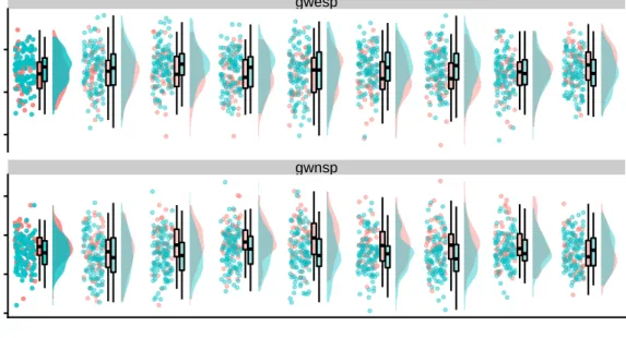
(Sec-edges gwesp gwnsp 40 80 120 50 100 150 200 40 60 80 100 s(Y)
Figure 2.3: A raincloud plot is a combination of a scatter plot, box plot, and density plot. Each dot in the scatter plot corresponds to a single observation, in this case, a network. The box plots depict the median (horizontal line), the interquartile range (box), and the most extreme values up to 1.5 times the interquartile range (vertical lines). The smoothed density plots augment the box plots by providing a more detailed view of the distribution of the data.
tion 2.4.4). To assess both the prior and the posterior, we make use of predictive checks. This necessitates the comparison of populations of networks, a somewhat challenging task. To this end, we make use of raincloud plots, introduced in Section 2.4.1.
2.4.1
Raincloud plots
To visualise the distribution of graph metrics of a population of networks, we use rain-cloud plots [8]. A rainrain-cloud plot is a combination of a scatter plot, box plot and density plot, and can be used to visualise the distribution of any univariate metric. Each dot in the scatter plot corresponds to a single observation, in this case, a network. The box plots depict the median (horizontal line), the interquartile range (box), and the most extreme values up to 1.5 times the interquartile range (vertical lines). The smoothed density plots augment the box plots by providing a more detailed view of the distribution of the data. See Figure 2.3 for a raincloud plot of the observed summary statistics (edges, GWESP, GWNSP) of the synthetic population of networks described in Section 2.3.1.
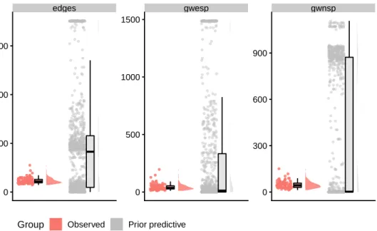
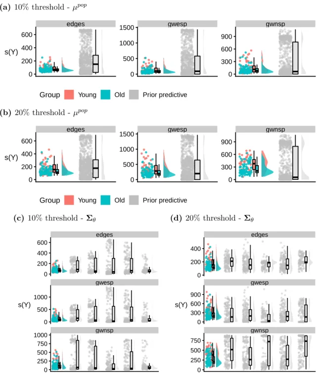
edges gwesp gwnsp 0 300 600 900 0 500 1000 1500 0 200 400 600 s(Y)
Group Observed Prior predictive
Figure 2.4: Prior predictive check forµ. The red plot corresponds to then = 100 networks of the synthetic dataset (see Section 2.3.1). The grey plot corresponds to 1000 networks generated under the prior predictive distribution. The range of prior predictive values covers those of the synthetic data, indicating an appropriate prior distribution.
2.4.2
Prior predictive checks
Given the complex geometry of exponential random graph models [115], it is important to verify that the prior distributions are appropriately specified. To do so, we perform prior predictive checks by simulating (populations of) networks from the prior and comparing them graphically to the observed data. Although this may be relatively straightforward for simple examples, it is rather more difficult for our model given its hierarchical struc-ture, and the challenge of comparing networks.
We check the prior specification in two stages. First, we assess whether the prior for the group-level mean parameterµgenerates exponential random graphs that are broadly similar to the observed networks in terms of the model summary statistics. Secondly, we check the prior for the group-level covariance parameter by comparing the variance of the observed summary statistics to populations of networks generated under the prior distribution. We now describe these two steps in greater detail.
samples from the prior predictive distribution for a single network:
πµ(y)∼
Z
π(y|µ)π(µ)dµ (2.22)
To do so, we first sample from the priorµi ∼π(µ) and then simulate a single exponential
random graph Yi ∼ERGM(µi).
To compare observed networks with the networks simulated from the prior predictive distribution, we use raincloud plots to visualise the distribution of the summary statistics of the respective networks. Figure 2.4 depicts the summary statistics of the synthetic dataset next to those of 1000 networks simulated from the prior predictive distribution under the conditionally conjugate prior µ ∼ N(0,100I). The networks generated under the prior predictive distribution exhibit a wide range of summary statistic values that cover those in the synthetic dataset, indicating that the prior is appropriately specified. Observe that the complexity of ERGMs is evidenced by the prior predictive distribution: a spherical prior in parameter space appears to correspond to a multimodal distribution in network space.
To check the suitability of the prior on the covariance parameter Σθ, we generate sets
of networks from the prior predictive distribution for apopulation of networks conditional on the hyperparameter µ0:
πµ(y)∼
Z
π(y|θ)π(θ)dθ. (2.23) This is done by first simulating Σθ ∼ W−1(νθ,Ψθ). We then generate n individual-level
parameters ˜θi ∼ N(µ0,Σθ) and, from each of these, generate an exponential random
graph Yi ∼ ERGM(θi). This process results in a population of networks that we can
contrast with the observed data.
Due to space limitations, it is difficult to plot more than a handful of simulated pop-ulations at once. As a result, we only plot up to 8 poppop-ulations (along with the observed data) selected to reflect the possible variability of the summary statistics within the pop-ulations generated under the prior (Figure 2.5). In this example, we set µ0 =µtrue. The
majority of the networks in the prior predictive populations (grey plots) have similar summary statistics to those of the synthetic data (red plot). Some of the populations, however, also contain networks with vastly different summary statistics, suggesting the prior is not overinformative.
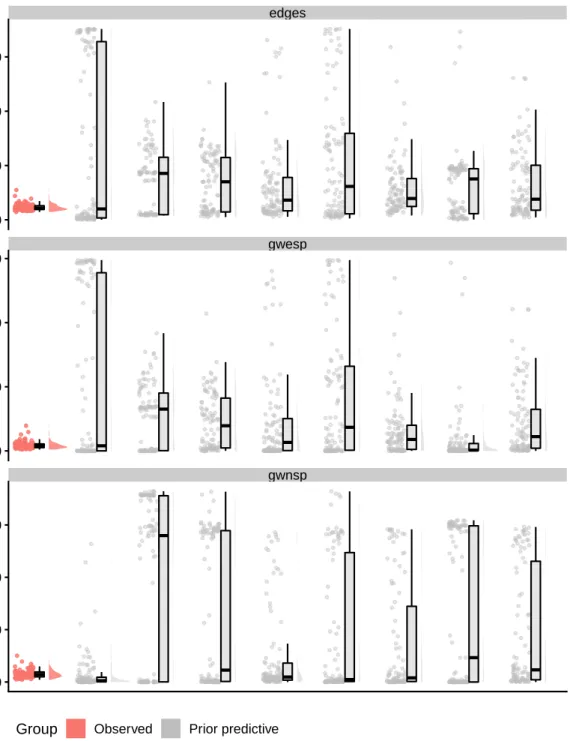
gwnsp gwesp edges 0 200 400 600 0 500 1000 1500 0 300 600 900 s(Y)
Group Observed Prior predictive
Figure 2.5: Prior predictive check for Σθ. The red plot corresponds to the n = 100
net-works of the synthetic dataset (see Section 2.3.1). The eight grey plots correspond to eight populations of n = 100 networks generated under the prior predictive distribution conditional on a fixed meanµ0 =µtrue. While the majority of the networks in the prior
predictive populations have similar summary statistics to those of the synthetic data, some also contain networks with vastly different summary statistics, suggesting the prior is not overinformative.
2.4.3
Convergence
The exchange-within-Gibbs algorithm produces a sequence of samples of the model pa-rameters (θ, φ) with the correct stationary distributionπ(θ, φ|y). Before we can reliably use these samples, however, we must first check that the sequence has converged. A key tuning parameter in the algorithm is the number of MCMC iterations K. The aim is to choose K large enough such that we can be confident that the sequence has converged, and have enough draws from the posterior to reliably estimate any quantity of interest.
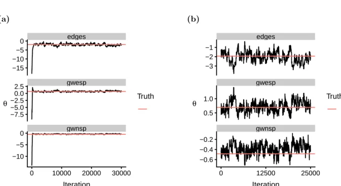
We assess convergence visually, using trace plots. By plotting the sequence of samples produced by an MCMC algorithm for a given model parameter, trace plots provide a way to check whether a given sequence has reached stationarity. We illustrate this with an example of a Bayesian ERGM fit to a single 38-node network from the synthetic dataset described in Section 2.3.1. To recap, this network was generated from an ERGM with three summary statistics (edges, geometrically weighted edgewise shared partners, and geometrically weighted non-edgewise shared partners) with corresponding parameter val-ues inspired by real brain connectivity networks. The generating parameter valval-ues for this particular network were θ = (−1.94,0.69,−0.49). Figure 2.6a displays the trace plot for the sequence of θ values produced by Algorithm 2.2.
In this example, we initialised the algorithm at θ0 = (−18.13,−9.31,−13.60), which was generated at random fromN(0,100I). For the first 2000 iterations or so, the sequence of samples appears to explore the parameter space before settling on the target distribu-tion π(θ|y). This initial period of iterations, known as burn-in, is highly influenced by the choice of starting values. To reduce their impact, we discard those iterations before the sequence appears to have converged. Figure 2.6b shows the trace plot for the same sequence of samples after discarding the first 5000 iterations.
Even if the sequence of samples produced by a model fitting procedure appears to have converged, this does not ensure that the samples are being drawn from the target distribution. For example, the sequence may be stuck in a local maximum of the distribu-tion. In the case of simulated data, we may check whether the distribution of the samples indeed covers the (known) true model parameter values. The density plots in Figure 2.7 confirm this in the case of the single Bayesian ERGM fit.
Once we are confident that we are drawing samples from the posterior distribution, we may compute theeffective sample size of the sequence for a given (univariate) parameter. If the samples from the algorithm were independent, then the effective sample size would simply be the number of iterations. However, in practice we have to account for the
(a) gwnsp gwesp edges 0 10000 20000 30000 −15 −10 −5 0 −7.5 −5.0 −2.5 0.0 2.5 −10 −5 0 Iteration θ Truth (b) gwnsp gwesp edges 0 12500 25000 −3 −2 −1 0.5 1.0 −0.6 −0.4 −0.2 Iteration θ Truth
Figure 2.6: (a) Trace plot depicting the sequence of samples produced by the model fitting procedure for a single Bayesian ERGM on a simulated network. After about 2500 itera-tions, the sequence of samples appears to converge around the true underlying parameter values. (b) The same trace plot after discarding the first 5000 iterations.
edges gwesp gwnsp −3 −2 −1 0 0.0 0.5 1.0 −1.0 −0.8 −0.6 −0.4 −0.2 0 1 2 0.0 0.5 1.0 1.5 2.0 0.0 0.2 0.4 0.6 θ Posterior density estimate Truth
Figure 2.7: The posterior density plot illustrates the kernel density estimate for the se-quence of samples produced by the fitting algorithm. In this case, the true values for all three model parameters are covered by the posterior density, suggesting that the samples are being drawn from the correct target distribution.
autocorrelation of the sequence of samples. To do so, we use theeffectiveSizefunction in the R package coda [110]. This estimates the effective sample sizeN∗ for a univariate parameter ψ as: N∗ =Nσˆ 2 ψ ˆ ρψ (2.24)
where ˆσψ2 is the variance of the sequence of ψ samples, ˆρψ is an estimate of the spectral
density at frequency zero of the sequence, and N is the number of MCMC iterations (after burn-in). A sequence with high autocorrelation will have a large value of σˆ
2
ψ
ˆ
ρψ and
so a comparably small effective sample size. Since each iteration of Algorithm 2.3 is computationally expensive, we would therefore prefer to construct sequences with low autocorrelation, in order to increase the effective sample size per MCMC iteration. We explore various approaches towards reducing autocorrelation in Section 2.5.
2.4.4
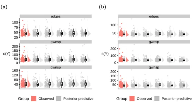
Posterior predictive checks
Having produced a sufficient number of samples from the posterior distribution, we then assess whether the model adequately describes the data. Since determining the distribu-tion of appropriate test quantities is difficult, assessing such goodness-of-fit for ERGMs is typically performed graphically [76]. For a single ERGM fit, one can simulate a large number of networks from the fitted model and compare these simulations to the observed network. This comparison is usually done via a set of network metrics. If a model fits the data well then the network metr