The University of Adelaide
School of Economics
Research Paper No. 2010-26
October 2010
Semiparametric Estimation in Simultaneous
Equations of Time Series Models
Semiparametric Estimation in
Simultaneous Equations of Time Series Models
Jiti Gao
School of Economics, University of Adelaide
Peter C. B. Phillips
Yale University, University of Auckland,
University of Southampton, & Singapore Management University
October 26, 2010
Abstract
A system of vector semiparametric nonlinear time series models is studied with possible dependence structures and nonstationarities in the parametric and nonparametric components. The parametric regressors may be endoge-nous while the nonparametric regressors are strictly exogeendoge-nous. The para-metric regressors may be stationary or nonstationary and the nonparapara-metric regressors are nonstationary time series. Semiparametric least squares (SLS) estimation is considered and its asymptotic properties are derived. Due to endogeneity in the parametric regressors, SLS is not consistent for the para-metric component and a semiparapara-metric instrumental variable least squares (SIVLS) method is proposed instead. Under certain regularity conditions, the SIVLS estimator of the parametric component is shown to be consistent with a limiting normal distribution. Interestingly, the rate of convergence in the parametric component depends on the properties of the regressors. It has been shown that the conventional rate–√n is still achievable even when nonstationarity is involved in both the regressors.
Key words and phrases: Dynamic simultaneous equation; endogeneity; exogeneity; non-stationarity; partially linear model; vector semiparametric regression.
1
Introduction
Existing studies show that both nonstationarity and nonlinearity are common fea-tures of much economic data. Modeling such data in a way that allows for possible nonstationarity helps to avoid dependence on stationarity assumptions and mixing conditions for all of the variables in the system. At present there is a large literature on parametric linear modeling of nonstationary time series and interest has primarily focused on time series with a unit root or near unit root structure (for an overview, see, for example, Phillips and Xiao, 1998, and the references therein). In practical work, much attention is given to multivariate systems and cointegration models. Inferential methods for these linear systems include both parametric (e.g., Johansen 1991; 1995, 2000) and semiparametric (see, for example, Phillips and Hansen 1990, Phillips 1991; 1995, Watson 1994) approaches.
In comparison with work on linear parametric models, there have been only a few studies of parametric nonlinear models with integrated variables. Park and Phillips (1988, 1989, 1999, 2001) introduced techniques for developing asymptotics for cer-tain classes of nonlinear nonstationary parametric systems and aspects of this work have been extended by P¨otscher (2004), de Jong (2004), Jeganathan (2004, 2008), and Berkes and Horv´ath (2006). Interest has also developed in nonparametric mod-eling methods to deal with nonlinearity of unknown form involving nonstationary variables. Existing studies in the field of nonparametric autoregression and cointe-gration estimation include Phillips and Park (1998), Karlsen and Tjøstheim (1998, 2001), Wang and Phillips (2009a, 2009b), Karlsenet al (2007), Kasparis and Phillips (2009), Cai, Li and Park (2009), Schienle (2009), and Phillips (2009). The last pa-per examines in a nonparametric setting spurious time series models of the type considered by Granger and Newbold (1974, 1977) in a linear parametric setting, for which the asymptotic theory was given in Phillips (1986, 1998).
Among the nonparametric studies of nonstationarity, two different mathemati-cal approaches have been developed. In one approach, a so-mathemati-called “Markov splitting technique” has been used in Karlsen and Tjøstheim (1998, 2001), and Karlsen et al
(2007) to model univariate time series with some kind of null–recurrent structure; and Chen et al (2008) consider univariate semiparametric regression modeling of null–recurrent time series, in which there is neither endogeneity nor heteroskedas-ticity. In the other approach, Phillips and Park (1998), Phillips (2009), and Wang and Phillips (2009a, 2009b) have developed ‘local–time’ methods to derive an asymp-totic theory for nonparametric estimation of univariate models involving integrated time series.
In the case of independent and stationary time series data, semiparametric re-gression models have been intensively studied for more than two decades and there is a wide literature (Robinson 1988; Linton 1995; Pagan and Ullah 1999; H¨ardle et al 2000; Yatchew 2003; Gao 2007; Li and Racine, 2007, among many others). In applied work, semiparametric methods have been shown to be particularly useful in modeling economic data in a way that retains generality where it is most needed while reducing dimensionality problems.
for nonstationarities and endogeneities within a vector semiparametric regression model. The null recurrent structure of integrated time series typically reduces the amount of time that such time series spend in the vicinity of any one point, thereby exacerbating the sparse data problem or “curse of dimensionality” in nonparametric and semiparametric modeling of multivariate integrated time series. On the other hand, recurrence means that nonlinear shape characteristics of unknown form may be captured over unbounded domains and endogeneity may be often accommodated without specialized methods (Wang and Phillips 2009b).
A common motivation for the use of semiparametric formulations such as (1.1) below is that they reduce nonparametric dimensionality through the presence of a linear parametric component. In our setting, the time series{(Yt, Xt, Vt) : 1≤t ≤n}
are assumed to be modeled in a system of simultaneous equations of the form
Yt=A Xt+g(Vt) +t,
Xt=H(Vt) +Ut, t= 1,2,· · ·, n,
E[t|Vt] =E[t] = 0 and E[Ut|Vt] = 0, (1.1)
where n is the sample size, A is a p ×d–matrix of unknown parameters, Yt =
(yt1,· · ·, ytp)0, Xt = (xt1, · · ·, xtd)0, and Vt is a sequence of univariate integrated
time series regressors, g(·) = (g1(·),· · ·, gp(·))0 and H(·) = (h1(·),· · ·, hd(·))01 are all
unknown functions, and both t and Ut are vectors of stationary time series. An
extended version of model (1.1) is given in (2.21) in Section 2.3 below to deal with a more general case.
Model (1.1) corresponds to similar structures that have been used in the inde-pendent case (see Linton 1995; Neweyet al 1999; Su and Ullah 2008). The condition
E[t|Vt] = E[t] is generally needed to ensure that the model is identified. For, if
there were an unknown functionλ(·) such thatt=λ(Vt)+εtwithE[εt|Vt] = 0,then
onlyg(·) +λ(·) would normally be estimable. However, recent research has revealed that some cases where t is correlated with Vt may be included. In particular, in
studying nonparametric regressions of the form Yt = g(Vt) +t, Wang and Phillips
(2009b) consider a nonstationary endogenous regressor case where Vt is correlated
with t and show that conventional nonparametric regression is applicable in spite
of the endogeneity. Phillips and Su (2010) show that the same phenomena holds in cross section cases where there are continuous location shifts in the regressor, which play the role of an instrumental variable in tracing out the nonparametric regression function.
The identification conditionE[t|Vt] =E[t] = 0 eliminates endogeneity between
t andVt while retaining endogeneity betweent andXt and potential
nonstationar-ity in both Xt and Vt. The condition E[t|Vt] =E[t] = 0 in our setting corresponds
to the condition E[t|Vt, Ut] = E[t|Ut] that is assumed in Newey et al (1999) and
Su and Ullah (2008), the former being implied by E[t|Vt] = E(E[t|Ut, Vt]|Vt) =
E(E[t|Ut]|Vt) =E(E[t|Ut]) =E[t] when Ut is independent ofVt and E[t] = 0.
The identification conditions in (1.1) allow for both conditional heteroskedasticity
1F0(·) denotes transpose of the vector functionF(·), andF(i)(·) denotes thei–th derivative of
and endogeneity int,permitting tto depend onUt2. These conditions are also less
restrictive than the exogeneity condition between t and (Xt, Vt) that is common in
the literature for the stationary case (see, for example, Gao 2007).
The present paper treats model (1.1) as a vector semiparametric structural model and considers the case whereXtandVtmay be vectors of endogenous, nonstationary
regressors. In the case where endogeneity is involved in semiparametric regression modeling of independent data, some related developments include Robinson (1988), Newey et al (1999), Ai and Chen (2003), Newey and Powell (2003), Blundell et al
(2007), Florens et al (2007), and Su and Ullah (2008). While estimation of partially linear models with endogeneity is discussed in each of these papers, neither the proposed structures nor the estimation methods may be used to deal with our case. The contributions of the paper are as follows. We first consider a semiparamet-ric least squares (SLS) estimator of A. When there is endogeneity in Xt, the SLS
estimator of A is inconsistent. Accordingly, the paper proposes a semiparametric instrumental variable least squares (SIVLS) estimate of A to deal with endogeneity in Xt and a nonparametric estimator for the function g(·). The SIVLS estimator
of A is shown to be consistent with a conventional√n–rate of convergence in some cases even whenXtis stochastically nonstationary. This rate arises because
nonsta-tionarity in the regression can be eliminated by means of stochastic detrending. The semiparametric procedure given here may be used on a system of non-linear simultaneous equations with the following features: (i) nonstationarity and endogeneity in the parametric regressors; (ii) nonlinearity and nonstationarity in the nonparametric regressors; and (iii) stationary residuals. As such, the paper complements existing results on parametric dynamic simultaneous equations mod-els (Zellner and Palm 1974; Hsiao 1997), parametric modeling with endogeneity (such as Phillips 1983; Sargan 1988), parameter estimation in simultaneous equa-tions models (such as Greene 2005), nonparametric and semiparametric estimation of nonlinear time series (such as Tong 1990; Fan and Yao 2003; Gao 2007), param-eter estimation in vector autoregression and cointegration (such as Watson 1994), instrumental variable estimation of nonparametric models (such as Robinson 1988; Newey et al 1999; Ai and Chen 2003; Newey and Powell 2003; Blundell et al 2007; Florens et al 2007; Su and Ullah 2008), and nonparametric and semiparametric es-timation of nonstationary time series (such as Phillips and Park 1998; Karlsen and Tjøstheim 2001; Karlsen et al 2007; Wang and Phillips 2009a, 2009b).
In comparison with a related paper by Chenet al (2008), who consider the case where{Vt}is a null recurrent Markov chain and assume the existence of an unknown
functional H(v) =E[Xt|Vt =v] that is independent of t in a scalar semiparametric
regression Yt = Xt0α +g(Vt) +t with E[t|Xt, Vt] = 0. By contrast, this paper
imposes a set of general conditions in Assumption 3.3 below on the integrated process
Vt. Note that a general integrated process is not a Markov chain unless it is of
the form Vt = Vt−1 + vt with vt being independent and identically distributed.
2The additive case where
t = λ(Ut) +µt with E[µt|Vt] = 0 is covered in the first part of (1.1) because E[t|Vt] = E[λ(Ut)|Vt] +E[µt|Vt] =E[λ(Ut)] = E[t] when Ut is independent of
Vt. The multiplicative case where t =σ(Ut)νt is also covered in the first part of (1.1) because
Other related studies include Cai, Li and Park (2009) for a nonstationary varying coefficient time series model, Gaoet al(2009a, 2009b) for model specification testing involving nonstationarity, and Phillips (2009) for nonparametric kernel estimation of the relationship between two integrated time series in a spurious regression model.
The paper is organized as follows. Section 2 proposes estimators of the parameter matrixAand the nonlinear functions g(·). Asymptotic results of the proposed semi-parametric estimators are established in Section 3. A bandwidth selection method is developed in Section 4.1. Section 4.2 gives two examples to illustrate implemen-tation. Conclusions are given and some limitations of the framework are discussed in Section 5. Proofs of the main results are given in Appendix A and subsidiary lemmas in Appendix B.
2
Semiparametric Estimation
Before addressing estimation, we provide more detailed discussion of the model and its implications. Write (1.1) in full as:
Yt =A Xt+g(Vt) +t (2.1)
Xt=H(Vt) +Ut, (2.2)
E[t|Vt] =E[t] = 0, (2.3)
E[Ut|Vt] = 0. (2.4)
When the variables {(Xt, Vt, t)}are jointly stationary with finite second moments,
the conditional expectation H(Vt) = E[Xt|Vt] is well–defined. It is common to
assume weak exogeneity, so that E[t|(Ut, Vt)] = 0, and letting Ut =Xt−E[Xt|Vt],
the decomposition of Xt = H(Vt) +Ut is immediate. In consequence, the model
(2.1)–(2.4) reduces to a standard semiparametric form
Yt=A Xt+g(Vt) +t, with E[t|(Ut, Vt)] = 0 (2.5)
as discussed, for example, in Robinson (1988), H¨ardle et al (2000) and Gao (2007). In the case where both Xt and Vt are nonstationary, the notion of a constant
conditional expectation functional E[Xt|Vt] may not be well defined. In (2.2), the
dependence of Xt on Vt takes the general form of a nonlinear cointegrating system
relating nonstationary variables. It follows from (2.1)–(2.4) that
E[Yt|Vt=v] = A H(v) +A E[Ut|Vt =v] +g(v) +E[t|Vt=v]
= A H(v) +g(v), (2.6) which implies that Ψ(v) =E[Yt|Vt=v] is well defined. In addition, (2.6) implies
g(v) = Ψ(v)−AH(v). (2.7)
Thus, in view of equation (2.7), we can rewrite (2.1) as
where et =t and Ut =Xt−H(Vt),as assumed in (1.1). Introducing the
“stochas-tically detrended” variable
Wt =Yt−Ψ(Vt), (2.8)
we can write (2.1) and (2.2) in semiparametrically contracted form as
Wt=A Ut+et. (2.9)
Regarding (2.6)–(2.9), we make the following observations:
• The contracted form model (2.9) is semiparametric because both Wt and Ut
are not observable and need to be estimated nonparametrically. • Since E[λtUt0] =E{λtE[Ut0|Vt]}= 0, we have
E[Ut0t] =E[Utλt0] +E[Ute0t] =E[Ute0t] =E[UtE(e0t|Ut)]. (2.10)
It follows that the unknown matrix A can be consistently estimated based on (2.9) when E[Ute0t] = 0. The following two cases show that this condition can still
be satisfied even when et may depend onUt.
Case 2.1. Consider a multiplicative relationship of the form et = σ(Ut)πt,
where πtis a sequence of independent random errors with E[πt|Ut] = 0 andσ(Ut) is
a positive definite matrix. In this case, we have E[et|Ut] =σ(Ut)E[πt|Ut] = 0.
Case 2.2. Letp(·) be the marginal density ofUtandγ(u) = E[e0t|Ut =u]. Then,
E[Ute0t] = E[UtE(e0t|Ut)] = E[Utγ(Ut)] = R−∞∞ uγ(u)p(u)du = 0 when γ(u)p(u) =
γ(−u)p(−u) for allu.
In such cases as these, there is no need to introduce instrumental variables (IVs) in the estimation of (2.9). Otherwise, endogeneity must be addressed and an IV procedure may be used to achieve consistent estimation of A.Section 2.1 proposes a semiparametric least squares (SLS) estimation method for the case whereE(e0t|Ut) =
0. Section 2.2 develops a semiparametric instrumental variable procedure (SIVLS) that is applicable in the case of nonstationary Ut.
2.1
SLS estimation
When E(e0t|Ut) = 0, consistent estimation is possible based on (2.9). But since both
WtandUtare unobservable, the unknown functions Ψ(·) andH(·) must be estimated
nonparametrically. Substituting nonparametric kernel estimates into (2.9) gives an approximate semiparametric nonlinear time series model of the form
e Yt =A Xft+et, (2.11) where Yet = Yt−Ψ(b Vt) Ft and Xft = Xt−Hc(Vt) Ft. In these formulae, Ft is
the indicator Ft = I(pbn(Vt)> bn) where bn is a sequence of positive numbers that
tend to zero as n → ∞, pbn(v) = 1 √ nh Pn s=1K Vs−v h , Ψ(b v) = Pn s=1wns(v)Ys and
c
H(v) = Pn
s=1wns(v)Xs withwns(·) being a sequence of probability weight functions
of the form wnt(v) = Kv,h(Vt) n P k=1 Kv,h(Vk) with Kv,h(Vt) = 1 hK V t−v h , (2.12)
in whichK(·) is a probability kernel function andhis a bandwidth parameter. Note that since Vt is scalar, we need only use a single bandwidth parameter h.
The semiparametric least squares (SLS) estimator ofAis defined by the equation
b
A=Ye0Xf(Xf0Xf)−1, (2.13)
where Xf0 = (Xf1,· · ·,Xfn), Ye0 = (Ye1,· · ·,Yen), and throughout the paper D−1 is
the inverse of D or a generalized inverse if D−1 does not exist. This type of
trun-cated least squares estimation method has been widely used in the literature for the independent sample case (see, for example, Robinson 1988).
The vector of unknown functionsg(·) is then estimated by
b g(v) =gn(v;Ab)≡ n X s=1 wns(v)Ys−Ab n X s=1 wns(v)Xs. (2.14) By elementary calculation (Ab−A) Xf0Xf=ee0Xf+Ge0X,f (2.15) with Ge0 = (Ge1,· · ·,Gen) = (ge(V1),· · ·,ge(Vn)), ge(Vt) = g(Vt)− n P s=1 wns(Vt)g(Vs), ee 0 = (ee1,· · ·,een) and eet = et− n P s=1
wns(Vt)es. This estimator in (2.13) is implemented in
Example 4.1 below.
Assuming that g(·) and H(·) are both differentiable and their first derivatives are all continuous, as shown in Appendix A, an approximate version of (2.15) has the form
(Ab−A) U0U (1 +oP(1)) =e0U (1 +oP(1)), (2.16)
where e0 = (e1,· · ·, en) and U = (U1,· · ·, Un)0. This reduction shows that
√
n
convergence is achievable when E[e|U] = 0 and some smoothness conditions are imposed on g(·) and H(·).
Equation (2.16) also shows that Ab will be inconsistent when U is a matrix of
endogenous regressors for which E[e|U] 6= 0. This case is now considered and a semiparametric instrumental variable least squares (SIVLS) estimation method for A is developed that is consistent and has desirable asymptotic distributional properties.
2.2
SIVLS estimation
In the case where U is a matrix of integrated regressors, a semiparametric version of the fully modified (FM) estimation procedure of Phillips and Hansen (1990) and
Phillips (1995) may be used to consistently estimate A. That approach may be considered for the case where both Xt and Vt are univariate integrated regressors
and are independent of each other. But when U is a matrix of stationary regressors, the FM method fails. We therefore propose here a semiparametric instrumental variable (SIV) approach.
To develop the SIV method, in the semiparametric model
Wt=AUt+et with E[et|Vt] = 0 and E[et|Ut]6= 0, (2.17)
we assume the existence of a vector of stationary variables ηt for which
E[Utηt0]6= 0 and E[et|ηt] = 0. (2.18)
Equations (2.17) and (2.18) imply
Wtηt0 =AUtηt0 +etη0t with E[Utηt0]6= 0 andE[etηt0] = 0. (2.19)
We focus on the case where the number of instruments equals the number of regres-sors and
rank ofE[η0η]≡r=d≡rank of E[η0U], (2.20) where η0 = (η1,· · ·, ηn). The case where the number of instrumental variables is
greater than the number of regressors may be analyzed in a similar way.
If Wt, Ut and ηt were all observed time series, models (2.17) and (2.19) would
consist of a system of vector semiparametric stationary IV time series models. Each
ηt may be regarded as the stationary component of a suitable IV. In this setting, it
is straightforward to construct a consistent estimator for A.
Since ηt may not be directly observable, we assume that there is a vector of
observed instruments, Qt, that satisfy an expanded version of the system (1.1) of
the form
Yt =A Xt+g(Vt) +t with E[t|Vt] =E[t],
Xt=H(Vt) +Ut with E[Ut|Vt] = 0,
Qt=J(Vt) +ηt with E[ηt|Vt] = 0, (2.21)
where ηt is assumed to satisfy (2.18), Qt = (qt1,· · ·, qtd)0 is a vector of possible
instrumental variables for Xt generated by a reduced form equation involving Vt,
and J(·) = (J1(·),· · ·, Jd(·))0 is a vector of unknown functions.
The residual ηt may be interpreted as a sequence of stochastically detrended
versions of Qt and we therefore assume thatηtis strictly stationary even though Qt
itself may be a vector of nonstationary instruments. In effect, the nonstationarity in Qt arises from the component J(Vt) which depends on the nonstationary process
Vt. It is particularly natural to choose a stationary IV likeηt as a residual when Ut
itself is assumed to be a stationary residual given by the stochastically detrended quantity Xt−H(Vt). The augmented system (2.21) simply adds in this instrument
generating equation to the original system (1.1). The new system obviously reduces to (1.1) when there is no endogeneity in Xt.
As discussed in the literature (see, for example, Li and Stengos 1996; Baltagi and Li 2002; Li and Racine 2007) for the stationary case, the existence and choice of Qt is often a difficult and important practical matter. In the nonstationary case,
similar considerations apply. To clarify the issues involved, we look at the following special case.
Remark 2.1. Consider a pair (et, ηt) of the form
et = Σ Ut+ ∆ Πt and ηt= ∆ Ut−Σ Πt, (2.22)
where both Σ and ∆ = I −Σ are deterministic, symmetric and positive definite matrices, and Πt is a vector of stationary errors satisfying E[Πt] = 0, cov(Ut,Πt) =
cov(Vt,Πt) = 0 and cov(Πt,Πt) = cov(Ut, Ut) = I. In this case, we have
E[etUt0] = ΣE[UtUt0], E[ηtUt0] = ∆E[UtUt0], E[etη0t] = ΣE[UtUt0] ∆ 0− ∆E[ΠtΠ0t] Σ 0 = 0. (2.23) We discuss how to estimate Σ. Using the linear reduced form (2.17) and substi-tuting (2.22) into (2.17), we have
Wt =A Ut+et = (A+ Σ) Ut+ (I−Σ)Πt=B Ut+ ∆ Πt, (2.24)
where B =A+ Σ and ∆ = I−Σ. Since cov(Ut,Πt) = 0, we can estimate B using
the same method as in (2.13) by Bb and the matrix Γ = ∆∆0 by
b Γ = 1 n n X t=1 e Yt−BbXft Yet−BbXft 0 . (2.25)
As shown in Corollary 3.3 below, we have Γb →P Γ asn → ∞. The matrix Σ is then
consistently estimated by Σ =b I−∆.b
Let J(v) = H(v). Then, Qt = J(Vt) + ηt is a vector of valid instrumental
variables. This case, along with the estimation method proposed in (2.25), is imple-mented in Example 4.2.
We now construct a consistent estimator for A. In view of equations (2.17)– (2.21), and similar to (2.13), we define the semiparametric instrumental variable least squares (SIVLS) estimator
b A∗ =Ab∗(h) =Ye0Qe f X0Qe −1 , (2.26) whereQe0 = (Qe1,· · ·,Qen), in whichQet=Qt−Pn s=1wns(Vt)Qs. Correspondingly, the
vector of unknown functions g(·) is estimated by
b g∗(v) = gn(v;Ab∗)≡ n X s=1 wns(v)Ys−Ab∗ n X s=1 wns(v)Xs. (2.27)
It follows from (2.26) that
(Ab∗−A)Xf0Qe = e
As shown in Appendix A, we have the following decomposition
(Ab∗−A) U0η (1 +oP(1)) =e0η (1 +oP(1)), (2.28)
where η= (η1,· · ·, ηn)0.
To establish the validity of the approximations given in (2.16) and (2.28), we impose certain regularity conditions which enable us to establish consistency and a limit distribution theory.
3
Asymptotic Theory
As pointed out in the Introduction, the limit theory in this kind of nonstationary semiparametric model depends on the probabilistic structure of the regressors and errors et, Ut, ηt and Vt as well as the functional forms of g(·), H(·) and J(·). It
is convenient for the development that follows to make general conditions on the nonstationary process Vt rather than specify a particular generating mechanism.
These conditions are discussed in Appendix A and include the usual integrated and near integrated process mechanisms that commonly appear in applications. It is also convenient to use mixing conditions to establish some of the main results in the paper and we recall that a matrix stationary process{Zt, t = 0,±1,· · ·}isα–mixing
if the mixing numbers α(n)→0 as n→ ∞, where
α(n) = sup
A∈F0
−∞,B∈Fn∞
|P(AB)−P(A)P(B)|, (3.1)
in which Fkj is the σ–field generated by {Zt, k≤t≤j}. For the original definition,
see Rosenblatt (1956).
The following assumptions are used to develop the asymptotic theory. A detailed discussion of these conditions is provided in Appendix A.
Assumption 3.1. (i) ξt = (Ut0, η
0
t)
0
is a vector of (strictly) stationary time series with E[ξ1] = 0 and E[kξ1k4+γ1] < ∞ for some γ1 > 0, where k · k denotes
the Euclidean norm. The process ξt is α–mixing with mixing numbers αξ(j) that
satisfy ∞ X j=1 α γ1 4+γ1 ξ (j)<∞. (3.2)
(ii) ζt =et or et ηt0 is a matrix of stationary time series with E[kζ1k4+γ2] <∞
for some γ2 >0. The process ζtis α–mixing with mixing numbersαζ(j)that satisfy
∞ X j=1 α γ2 4+γ2 ζ (j)<∞. (3.3)
Assumption 3.2. (i) Let model (1.1) hold and Qt be a vector of instrumental
variables such that conditions (2.18), (2.20) and (2.21) are all satisfied.
(ii) E[es+t ⊗ηt] = 0 for all s ≥ 0 and E[es⊗et⊗ηu ⊗ηv] = 0 when at least
(iii) Γ1 =E[U1η10] be nonsingular. (iv) Σ∗1 =I⊗Γ−11 Ω∗1 I⊗Γ−110 and Ω∗1 =P∞ j=0E h e1e01+j ⊗η1η1+0 j i
are positive definite.
Assumption 3.3. (i) {Vt:t≥0} is independent of {(et, Ut, ηt) :t≥1}.
(ii) If fi,k(·) is the density function of Vi,k = ϕi−k(Vi−Vk) for i > k with
ϕm = L√s(mm) for m≥1, where Ls(·) is a slowly varying function, then
inf
δ>0lim supm→∞ supi≥1
sup
|v|≤δ
fi+m,i(v)<∞. (3.4)
There exists a filtration {Ft, t ≥ 0} such that Vt is adapted to Ft and for which,
with probability one,
inf
δ>0lim supm→∞ supi≥1
sup
|v|≤δ
fi+m,i(v|Fi)<∞, (3.5)
where fi,k(v|Fk) is the conditional density function of Vi,k given Fk.
Assumption 3.4. (i)The vector function g(v)is continuously differentiable for
v ∈R and the derivative g(1)(v) satisfies, for large enough n,
n X t=1 Z g (1)(ϕ−1 t v) 2 ft,0(v)dv=O(nh−1), (3.6)
where {ft,0(v)} is as defined in Assumption 3.3 above.
(ii) The vector function H(v) is continuously differentiable for v ∈ R and the derivative H(1)(v) satisfies for large enough n
n X t=1 Z ||H(1)(ϕ−t1v)||2 f t,0(v)dv=O(nh−1) and (3.7) n X t=1 Z g(1)(ϕ−t1v)0H(1)(ϕ−t1v) ft,0(v)dv=O n12−ε1b2 nh −2 , (3.8)
where 0< ε1 < 12 is some constant.
(iii)The vector function J(v)is continuously differentiable for v ∈R with deriva-tive J(1)(v) that satisfies for large enoughn
n X t=1 Z ||J(1)(ϕ−t1v)||2 f t,0(v)dv=O(nh−1) and (3.9) n X t=1 Z g(1)(ϕ−t1v)0J(1)(ϕ−t1v) ft,0(v)dv=O n12−ε2b2 nh −2 , (3.10)
where 0< ε2 < 12 is some constant.
Assumption 3.5. (i)K(·) is a symmetric and bounded probability density
(ii) The sequences {hn} and {bn} both satisfy, as n → ∞, the following rate conditions hn →0, nh2n→ ∞, nh 6 n →0, (3.11) bn→0, Ls(n) √ nb2 n →0, L 2 s(n) √ h b2 n →0, L 6 s(n) nh2b8 n →0, (3.12)
where Ls(n) is as defined in Assumption 3.3(ii).
(iii) bn is chosen such that n
P
t=1
P (pbn(Vt)≤bn) = o(n).
(iv)There exists a real function λ(x, y)such that ||g(x+yh)−g(x)|| ≤hλ(y, x)
for small enough h, all y ∈ R = (−∞,∞) and R∞
−∞λ(x, y)K(x)dx < ∞ for any given y.
Some discussion and technical justifications for Assumptions 3.1–3.5 are provided in Appendix A. Under these conditions, we have the following results, whose proofs are also given in Appendix A.
Theorem 3.1 Under Assumptions 3.1, 3.2, 3.3, 3.4 and 3.5(i)(ii)(iii), as n→ ∞,
we have √ n(Ab∗−A)→D N(0,Σ∗ 1), (3.13) where Σ∗1 = I⊗Γ−11 Ω∗1 I⊗Γ−110 with Ω∗1 = P∞ j=0E h e1e01+j ⊗η1η1+0 j i and Γ1 =E[U1η01].
Theorem 3.1 shows that the semiparametric IV estimator Ab∗ can be
asymptot-ically normal in the limit even when the parametric and nonparametric regressors are both nonstationary. In addition, Ab∗ is consistent when there is endogeneity in
the parametric regressors. The explanation for the √n convergence rate and the limiting normality is that A is estimated based on (2.17) and (2.18), which consist of a system of vector semiparametric stationary IV time seres models in which ηt is
a vector of stochastically detrended versions of the instruments Qt. Stationarity of
(Ut, et, ηt) then ensures that standard asymptotic normality with a conventional
√
n
convergence rate is achievable.
When Xt is strictly exogenous and Ut is independent of et, Theorem 3.1 has the
following corollary.
Corollary 3.1 (i) Let Assumptions 3.1, 3.2, 3.3, 3.4(i)(ii) and 3.5(i)(ii)(iii) hold. Then as n → ∞ √ n(Ab−A)→D N(0,Σ∗ 1), (3.14) where Σ∗1 = I⊗Γ−11Ω1∗I⊗Γ−11 with Ω∗1 = P∞ j=0E h e1e01+j i ⊗EhU1U1+0 j i and Γ1 =E[U1U10].
(ii) If, in addition, both Ut and et are independent and identically distributed,
then as n→ ∞ √ n(Ab−A)→D N 0,Σ11⊗Σ−221 , (3.15) where Σ11=E[e1e01] and Σ22=E[U1U10].
Corollary 3.1 extends existing results for the univariate case where both the parametric and nonparametric regressors are independent random variables (see, for example, Robinson 1988; H¨ardle et al 2000) to the vector case where both the parametric and nonparametric regressors may be nonstationary. Chen et al (2008) obtain the univariate version of Corollary 3.1 under the assumption thatVtis a null
recurrent Markov chain.
Note that when there is heteroskedasticity inet, eitherAb orAb∗ may be replaced
by a weighted semiparametric least squares estimator (see, for example Chapter 2 of H¨ardle et al 2000). In this case, it is necessary to estimate the covariance matrix Ω∗1 by suitable application of some existing methods (see, for example, Andrews 1991; Phillips 1995). Such extensions are straightforward and are not considered here.
Recall that the nonparametric component is estimated by gb
∗(v) as defined in
(2.27). The asymptotic distribution of gb
∗(v) is obtained along lines similar to those
in Wang and Phillips (2009a) and Karlsen et al (2007) and is given in Theorem 3.2 below.
Theorem 3.2 Let the conditions of Theorem 3.1 hold. If, in addition, Assumption
3.5(iv) holds, then as n → ∞
v u u t n X t=1 K v−V t h (gb ∗ (v)−g(v))→D N(0,Ωg), (3.16) where Ωg = R K2(u)du·E[e 1e01] and λs() =E[s].
Remark 3.2. The random normalization in (3.16) implies that the convergence
rate depends on the order of the sample average Pn
t=1K v−V t h . In the stationary case, this quantity typically has order nh, whereas when Vt is a unit root or near
integrated process it has order √nh (see Wang and Phillips, 2009a). It follows that in the nonstationary case, the rate of convergence of gb
∗(v) is (√nh)12.
Finally, we establish the following convergence results for the residual moment matrix.
Theorem 3.3 Let Assumptions 3.1, 3.2, 3.3, 3.4 and 3.5(i)(ii)(iii) hold. If, in
addition, Σ11=E[e1e01] is positive definite, then as n→ ∞
b Σ11= 1 n n X t=1 Yt−Ab∗Xt−gb∗n(Vt) Yt−Ab∗Xt−bgn∗(Vt) 0 →P Σ11. (3.17)
Since Πtinvolved in (2.22) satisfies the same conditions as{(et, Ut)}, Theorem 3.3
can be used to deduce the following corollary when cov(Ut,Πt) = 0. The Corollary
below shows that the covariance matrix Σ involved in (2.22) representing the level of endogeneity in that model can be consistently estimated.
Corollary 3.2 Let Assumptions 3.1, 3.2, 3.3, 3.4(i)(ii) and 3.5(i)(ii)(iii) hold. If, in addition, Σ is positive definite, then as n→ ∞
b Γ = 1 n n X t=1 e Yt−BbXft Yet−BbXft 0 →P Γ (3.18)
when cov(Πt,Πt) = cov(Ut, Ut) =I, where Bb is as defined in (2.25) and Γ = ∆∆0.
Remark 3.3. As in other nonparametric and semiparametric estimation
prob-lems, bandwidth parameter choice is critical in the practical implementation of the proposed estimation procedure. In the case where Vt is stationary, existing studies
(see, for example,§2.1.3 of H¨ardleet al 2000) may be used to provide solutions. Sec-tion 4.1 proposes a semiparametric cross–validaSec-tion selecSec-tion method and provides some examples of its implementation.
4
Examples of Implementation
4.1
Bandwidth parameter choice
As in other nonparametric and semiparametric contexts, bandwidth choice is im-portant in practical implementation. In the case where Vi is stationary, many
ex-isting studies (see, for example, §2.1.3 of H¨ardle et al 2000) offer solutions. But in nonstationary regressor cases, the literature on bandwidth selection is limited (see, however, the discussion in Wang and Phillips, 2009a) and many issues are still to be investigated. The present section provides some discussion of the issue in the semiparametric setting considered here.
We start by introducing the leave–one–out estimators ofH(v), Ψ(v) and g(v) as follows: f Ht(Vt) = n X s=1,6=t Wns(−t)(Vt)Xs and Ψet(Vt) = n X s=1,6=t Wns(−t)(Vt)Ys, (4.1) gtn(Vt;A) = n X s=1,6=t Wns(−t)(Vt)(Ys−AXs) = Ψet(Vt)−A Hft(Vt), (4.2) whereW(−t) ns (Vt) = K(Vs−hVt) n P k=1,6=t K Vk−Vt h
. We then define the leave–one–out semiparametric
instrumental variable least squares (SIVLS) estimator of A by
e A=Ae(h) =Y 0 Q(X0Q)−1, (4.3) where X0 = (X1,· · ·, Xn),Xt = Xt−Hft(Vt) Ft = Xt− n P s=1,6=t W(−t) ns (Vt)Xs ! Ft, Q0 = (Q1,· · ·, Qn), Qt = Qt−Jet(Vt) Ft = Qt− n P s=1,6=t W(−t) ns (Vt)Qs ! Ft, Y 0 = (Y1,· · ·, Yn) and Yt = Yt−Ψet(Vt) Ft = Yt− n P s=1,6=t Wns(−t)(Vt)Ys ! Ft, in which Ft=I pn,t(Vt)> bn with pn,t(Vt) = √1nhPns=1,6=tK Vs−Vt h .
The corresponding leave–one–out estimator ofg(·) is obtained as
e
The leave–one–out cross–validation (CV) function is defined CV(h) = 1 n n X t=1 Yt−AXe t− e gt(Vt) 0 Yt−AXe t− e gt(Vt) , (4.5)
where get(Vt) = gtn(Vt;Ae). The optimal smoothing parameter he is then chosen so
that
CV(eh) = min
h∈Hn
CV(h), (4.6)
whereHnis a set of smoothing parameter values. The corresponding data-determined
estimators of A and g(·) are then given by
e
A∗ =Ae(eh), and e
g∗(v) =gn(v;Ae(eh)), (4.7)
where gn(v;A) is defined in (2.14).
The following examples show how to implement the proposed procedure. Through-out these examples, use K(x) = 12I[−1,1](x), and the optimal bandwidth eh is chosen
as shown above.
4.2
Simulated examples
Example 4.1 below demonstrates how the functional forms of g(·) and H(·) may affect the rate of convergence of Ab in the exogenous case. In this case, ηt =Ut and
J(·) = H(·). The following discussion looks at two pairs of (G(·), H(·)) such that the conditions in Assumption 3.4(i)(ii) are satisfied.
Example 4.2 examines an endogenous case where the parametric variables are linearly correlated with the detrended residuals. The estimation method proposed in Section 2.2 is implemented.
Example 4.1. Consider the semiparametric simultaneous equation model
Yt=A Xt+G(Vt) +t, (4.8)
where A is a matrix of 2×2 of unknown parameters of the form
A= a11 a12 a21 a22 = −0.5 0.6 0.6 −0.5 ,
Xt = (Xt1, Xt2)0 is a vector of time series regressors, Vt is a sequence of integrated
time series regressors of the form Vt = Vt−1 +vt with V0 = 0 and vt is a sequence
of stationary disturbances generated by vt = γ vt−1 +νt, for t = 1,2,· · ·, where
γ = 0, 0.5,0.9, v0 = 0 and νt is a sequence of independent errors generated from
N(0,1), G(·) = (g1(·), g2(·))0 is a vector of unknown functions, and t is a vector of
stationary time series errors generated from
t∼N 0 0 , 1 −0.6 −0.6 1 . (4.9)
Independently from t, generate Ut as Ut = 0.3 0 0 −0.3 Ut−1+µt, t= 1,2,· · ·, (4.10)
where U0 = (0,0)0 and µt is a vector of i.i.d. normal errors of the form
µt∼N 0 0 , 1 0.5 0.5 1 . (4.11)
We use the following functions in the model specification:
g1(v) = sin(v), g2(v) = cos(v) and H1(v) =H2(v) =v. (4.12)
The process Xt is generated by Xt=H(Vt) +Ut and Yt is generated by (4.8). The
proposed estimation method in Section 2.1 is then applied to estimate A, and G(·) and H(·). We assess finite sample performance using the measures
ASE1 = |ab11−a11|, ASE2 =|ba12−a12|,
ASE3 = |ab21−a21|, ASE4 =|ba22−a22|,
where abij is the (i, j)–th element of Ab.
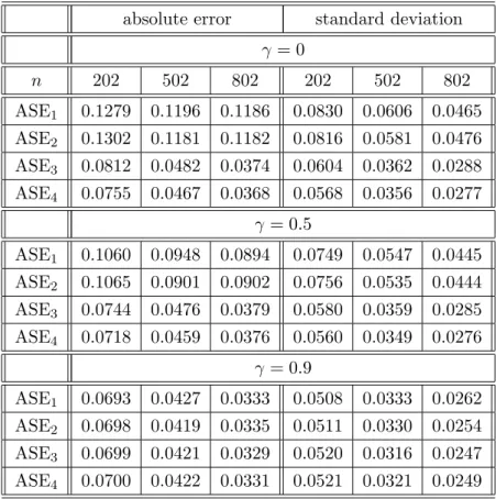
Table 4.1. Simulation results based on model (4.8)
absolute error standard deviation
γ = 0 n 202 502 802 202 502 802 ASE1 0.1279 0.1196 0.1186 0.0830 0.0606 0.0465 ASE2 0.1302 0.1181 0.1182 0.0816 0.0581 0.0476 ASE3 0.0812 0.0482 0.0374 0.0604 0.0362 0.0288 ASE4 0.0755 0.0467 0.0368 0.0568 0.0356 0.0277 γ = 0.5 ASE1 0.1060 0.0948 0.0894 0.0749 0.0547 0.0445 ASE2 0.1065 0.0901 0.0902 0.0756 0.0535 0.0444 ASE3 0.0744 0.0476 0.0379 0.0580 0.0359 0.0285 ASE4 0.0718 0.0459 0.0376 0.0560 0.0349 0.0276 γ = 0.9 ASE1 0.0693 0.0427 0.0333 0.0508 0.0333 0.0262 ASE2 0.0698 0.0419 0.0335 0.0511 0.0330 0.0254 ASE3 0.0699 0.0421 0.0329 0.0520 0.0316 0.0247 ASE4 0.0700 0.0422 0.0331 0.0521 0.0321 0.0249
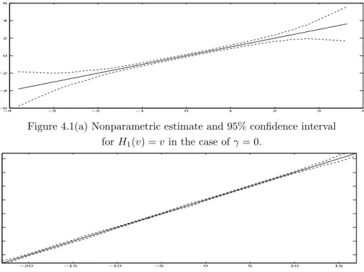
−4 −3 −2 −1 0 1 2 3 4 −6 −4 −2 0 2 4 6
Figure 4.1(a) Nonparametric estimate and 95% confidence interval forH1(v) =vin the case ofγ= 0.
−20 −15 −10 −5 0 5 10 15 −20 −15 −10 −5 0 5 10 15
Figure 4.1(b) Nonparametric estimate and 95% confidence interval forH1(v) =vin the case ofγ= 0.5.
The simulation results for both the absolute errors and standard deviations given in Table 4.1 were performed 1000 times and the means are tabulated in Table 4.1. In the case of (4.12), the conditions of Theorem 3.1 all hold. Table 4.1 provides the finite sample evidence relating to the limit theory of Theorem 3.1 for both stationary nonparametric regressors and integrated nonparametric regressors. In addition, Table 4.1 shows that the dependence structure of vt has some effect on
the rate of convergence, particularly in the integrated case and when γ is as large as 0.9.
For i = 1,2 and 1 ≤ j ≤ 1000, let Hci,j(·) be the estimate of Hi(·) at the j–th
replication, V(1)(j)≤V(2)(j)≤ · · · ≤V(n)(j) be the order statistics ofVt at thej–th
replication, Hci(·) = 1 1000
P1000
j=1 Hci,j(·) and V(t) = 10001 P1000j=1 V(t)(j). Figures 4.1(a)
shows a plot for Hc1 and its 95% confidence interval (CI) against (V(1),· · ·, V(n)) for
γ = 0 and n = 502, and Figure 4.1(b) shows a plot for Hc2 and its 95% confidence
interval against (V(1),· · ·, V(n)) forγ = 0.5 and n = 502.
Example 4.2. We consider a vector simultaneous equations model of the form
Yt=A Xt+G(Vt) +t, (4.13)
where A is a matrix of 2×2 of unknown parameters of the form
A= a11 a12 a21 a22 = 1.0 0.6 0.6 1.0 ,
Xt = (Xt1, Xt2)0 is a vector of time series regressors, Vt is a sequence of integrated
time series regressors of the form Vt = Vt−1 +vt with V0 = 0 and vt a sequence
of stationary disturbances generated by vt = γ vt−1 +νt, for t = 1,2,· · ·, where
γ = 0.1,0.5,0.9, v0 = 0 and νt is a sequence of independent errors generated from
N(0,1),G(·) = (g1(·), g2(·))0 is a vector of unknown functions, andtis generated by
t =ρ Ut+µt with values ofρ taken from {0,0.5,0.9} and whereµt and Ut are two
vectors of stationary time series errors independently generated as µt ∼ N(0, I2)
and Ut ∼N(0, I2).
Choose J(v) = H(v) and the following functions:
g1(v) = cos(v), g2(v) = sin(v), H1(v) = vcos(v), H2(v) =vsin(v). (4.14)
The process Xt followsXt=H(Vt) +Ut and Yt is generated by (4.13). We estimate
A by Ab∗ of (2.26) with the choice ofQt=J(Vt) +ηt and ηt =Ut−ρ µt, in which ρ
is estimated by (2.25) in computing Ab∗ and (4.15) below.
The simulation results for both the absolute errors and standard deviations are based on 1000 replications and the means of the following quantities are tabulated in Tables 4.2–4.4: ASE∗1 = |ab ∗ 11−a11|, ASE∗2 =|ba ∗ 12−a12|, ASE∗3 = |ab ∗ 21−a21|, ASE∗4 =|ba ∗ 22−a22|, (4.15) where ab ∗ ij is the (i, j)–th element of Ab ∗.
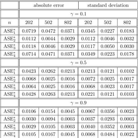
Table 4.2. Simulation results based on model (4.13) withρ= 0
absolute error standard deviation
γ = 0.1 n 202 502 802 202 502 802 ASE∗1 0.0719 0.0472 0.0371 0.0345 0.0227 0.0183 ASE∗2 0.0112 0.0044 0.0029 0.0112 0.0046 0.0032 ASE∗3 0.0118 0.0046 0.0029 0.0117 0.0050 0.0030 ASE∗4 0.0714 0.0471 0.0371 0.0349 0.0223 0.0178 γ = 0.5 ASE∗1 0.0423 0.0262 0.0213 0.0213 0.0121 0.0102 ASE∗2 0.0068 0.0025 0.0016 0.0072 0.0025 0.0017 ASE∗3 0.0064 0.0025 0.0016 0.0068 0.0023 0.0017 ASE∗4 0.0428 0.0263 0.0213 0.0221 0.0121 0.0103 γ = 0.9 ASE∗1 0.0106 0.0154 0.0045 0.0067 0.0356 0.0023 ASE∗2 0.0030 0.0094 0.0003 0.0037 0.0293 0.0003 ASE∗3 0.0029 0.0105 0.0003 0.0040 0.0352 0.0003 ASE∗4 0.0105 0.0167 0.0045 0.0068 0.0484 0.0022
Table 4.3. Simulation results based on model (4.13) with ρ= 0.5
absolute error standard deviation
γ = 0.1 n 202 502 802 202 502 802 ASE∗1 0.0741 0.0464 0.0378 0.0358 0.0222 0.0182 ASE∗2 0.0129 0.0051 0.0033 0.0130 0.0051 0.0035 ASE∗3 0.0128 0.0048 0.0032 0.0132 0.0045 0.0033 ASE∗4 0.0733 0.0466 0.0378 0.0358 0.0225 0.0182 γ = 0.5 ASE∗1 0.0420 0.0276 0.0211 0.0219 0.0138 0.0106 ASE∗2 0.0069 0.0029 0.0018 0.0071 0.0029 0.0018 ASE∗3 0.0072 0.0030 0.0018 0.0077 0.0030 0.0018 ASE∗4 0.0417 0.0278 0.0210 0.0220 0.0136 0.0103 γ = 0.9 ASE∗1 0.0103 0.0058 0.0044 0.0059 0.0033 0.0022 ASE∗2 0.0016 0.0017 0.0004 0.0017 0.0021 0.0004 ASE∗3 0.0016 0.0016 0.0004 0.0017 0.0022 0.0004 ASE∗4 0.0102 0.0059 0.0044 0.0059 0.0034 0.0022
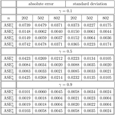
Table 4.4. Simulation results based on model (4.13) with ρ= 0.9
absolute error standard deviation
γ = 0.1 n 202 502 802 202 502 802 ASE∗1 0.0739 0.0479 0.0371 0.0373 0.0227 0.0175 ASE∗2 0.0148 0.0062 0.0040 0.0150 0.0061 0.0044 ASE∗3 0.0149 0.0059 0.0037 0.0152 0.0064 0.0036 ASE∗4 0.0742 0.0478 0.0371 0.0365 0.0223 0.0174 γ = 0.5 ASE∗1 0.0423 0.0269 0.0212 0.0223 0.0134 0.0105 ASE∗2 0.0084 0.0034 0.0020 0.0088 0.0035 0.0020 ASE∗3 0.0083 0.0033 0.0021 0.0085 0.0033 0.0021 ASE∗4 0.0425 0.0268 0.0214 0.0232 0.0135 0.0105 γ = 0.9 ASE∗1 0.0101 0.0060 0.0045 0.0058 0.0034 0.0024 ASE∗2 0.0019 0.0018 0.0004 0.0021 0.0023 0.0004 ASE∗3 0.0019 0.0018 0.0004 0.0020 0.0022 0.0004 ASE∗4 0.0103 0.0058 0.0045 0.0058 0.0035 0.0024
−3 −2 −1 0 1 2 3 −2 −1.5 −1 −0.5 0 0.5 1
Figure 4.2(a) Nonparametric estimate and 95% confidence interval for g1(v) = cos(v) in the case of ρ=γ = 0.
−3 −2 −1 0 1 2 3 −1 −0.5 0 0.5 1 1.5 2
Figure 4.2(b) Nonparametric estimate and 95% confidence interval for g2(v) = sin(v) in the case of ρ=γ = 0.
The absolute errors and the standard deviations in Tables 4.2–4.4 together show that the proposed estimation method performs well for the linear endogenous case where
Yt=AXt+G(Vt) +t and t=ρUt+µt, (4.16)
whereUt andµtare vectors of mutually independent time series errors. In addition,
the results show that the proposed estimation method is quite robust with respect to the values of γ and ρ.
For i = 1,2 and 1 ≤ j ≤ 1000, let gbi,j(·) be the estimate of gi(·) at the j–
th replication, V(1)(j) ≤ V(2)(j) ≤ · · · ≤ V(n)(j) be the order statistics of Vt at
the j–th replication, gbi(·) = 1 1000 P1000 j=1 gbi,j(·) and V(t) = 1 1000 P1000 j=1 V(t)(j). Figures
4.2(a) shows a plot for bg1 and its 95% confidence interval against (V(1),· · ·, V(n)) for
ρ=γ = 0 andn = 502, and Figure 4.2(b) shows a plot forgb2 and its 95% confidence
interval against (V(1),· · ·, V(n)) forρ=γ = 0.5 and n= 502.
5
Conclusions and Discussions
This paper explores the semiparametric estimation of a finite dimensional parameter matrix and nonparametric function estimation in the context of a multiple equa-tion nonlinear simultaneous equaequa-tions model of the form (1.1) in which stochastic trends of unknown form may be present. The proposed semiparametric instrumen-tal variable (SIV) least squares procedure addresses endogeneity in the parametric
regressors and enables asymptotically consistent estimation of the nonparametric functions.
The framework here extends univariate semiparametric regression with both in-dependent and stationary regressors and errors to a general multivariate case where both the parametric and nonparametric regressors may be nonstationary. A non-parametric kernel estimation method has been used to eliminate the nonlinear com-ponents and construct an approximating parametric model which leads to the SIV estimator. The SIV estimator resolves endogeneity in the parametric regressors in a semiparametric setting that allows for possible stochastic trends in the generating mechanism for both the endogenous and exogenous regressors, thereby making the model and method relevant for many potential applications in which the regressors may be endogenous, stochastic trends may be present in the data, and nonlineari-ties may occur in the generating mechanism. Simulations reveal that the proposed estimation method is easily implemented in practice and performs well in relation to the asymptotic theory for moderately sized samples.
While the nonparametric stochastic detrending approach explored here has the advantage of imposing only weak conditions on the trend functions, the √n conver-gence rate is below the usual n rate for cointegrated system estimation and may be improved in some cases. Consider, for example, the system
Yt = a Xt+b g(Vt) +t with g(Vt) = 1 1 +V4 t , (5.1) Xt = H(Vt) +Ut and H(Vt) = c Vt, (5.2)
with Vt =Pts=1vs, where all variables are scalar and satisfy the conditions of
The-orem 3.1. In this case, the simple IV estimator aIV = (Pnt=1XtVt)
−1
(Pn
t=1VtYt)
converges at the usual rate nfor cointegrated systems and has a mixed normal limit distribution that is amenable to inference. To see this, we use the following three results (the first two are standard and the third follows from the limit theory for a zero energy functional of a partial sum process – see Jeganathan, 2008):
1 n2 n X t=1 XtVt ⇒ c Z 1 0 Bv2, 1 n n X t=1 Vtt ⇒ Z 1 0 BvdB, 1 q√ n n X t=1 Vt 1 +V2 t ⇒ qβ L1 0 Z, where √1 n P[n·]
t=1(t, vt) ⇒ (B, Bv), bivariate Brownian motion, L10 = L1Bv(1,0) is
the local time of Bv at the origin over the unit time interval [0,1],Z is a standard
normal variate, and the constant β depends on the distribution of the {vt}. From
these results, we have the limit theory
n(aIV −a) = c Z 1 0 Bv2 −1Z 1 0 BvdB ,
which has a mixed normal distribution under the exogeneity condition onVt.In this
case, direct IV estimation is (asymptotically infinitely) superior to semiparametric estimation involving nonparametric stochastic detrending. Models (5.1) and (5.2) are of some practical interest. In particular, the function g(Vt) is integrable and
provides a ‘small’ nonlinear correction to the linear component of the cointegrating relation (5.1). This nonlinear component becomes most relevant when the process
Vt takes values near the origin but the function could easily be reformulated so
that the most relevant values occured elsewhere in the sample space. The remain-ing components of the system are analogous to those in conventional cointegrated systems. Thus, (5.1) - (5.2) is a cointegrated system with small deviations from linearity that affect the relationship but do not disturb the properties of a simple IV estimator. In effect, estimation of the linear component aXt may be conducted
without concern for the nonlinear component. So nonlinear stochastic detrending is unnecessary here. Of course, when the functional form of the stochastic trending component is unknown then a parametric procedure like linear IV estimation may be unreliable and will normally result in inconsistency.
A further limitation is the assumption of exogeneity for the nonstationary regres-sor Vt. It will be useful to relax this condition in applications to allow the trending
mechanism to be endogenous. A final limitation of the model is that each compo-nent of g(·) is a scalar function of Vt. For practial work, it will often be useful for
g(·) to be a function of several regressors involving both stationary and integrated components. These issues require different treatment of the asymptotic theory and some extension of the methods discussed here, so they are left for future research.
6
Acknowledgments
This work was started when the first author was visiting the Cowles Foundation for Research in Economics at Yale University between September and November 2007. The work of the first author was supported financially by the Cowles Founda-tion and two Australian Research Council Discovery Grants under Grant Numbers: DP0879088 and DP1096374. The work of the second author was supported by the Kelly Foundation and the NSF under Grant Number: SES 06–47086. The first author would also like to acknowledge useful discussions with Xiaohong Chen and Yuichi Kitamura while visiting Yale University. Thanks from the first author also go to Jiying Yin for his excellent computing assistance.
Jiti Gao, School of Economics, The University of Adelaide, Adelaide SA 5005, Australia. Email: [email protected].
Peter C B Phillips, Cowles Foundation for Research in Economics, Yale University, New Haven, CT 06520, USA. Email: [email protected].
7
Appendix A
7.1
Discussion of Assumptions 3.1–3.5Assumption 3.1 is quite general allowing for a stationary dependence structure for ξt and
ζt. Under some additional technical conditions, these time series might be stationary linear
processes that are also α–mixing (see Corollary 4 of Withers 1981 for example).
Assumption 3.2(i) is needed to ensure thatQtis a vector of valid instrumental variables
when E[et⊗ηt]6= 0. Assumption 3.2(ii) is needed to deal with quadratic forms involving
es and ηt. As pointed out in the beginning of Section 2.2, ηt is a vector of stationary
detrended errors. Thus, it is not unreasonable to require ηt to be stationary, althoughQt
can be nonstationary. Assumptions 3.2(ii)–(iv) are needed for the main theorems.
Assumption 3.3(i) imposes independence betweenVt and (es, Us, ηs). Since (es, Us, ηs)
is a vector of stochastically detrended stationary errors on the one hand and Vt is a
sequence of nonstationary errors on the other hand, it is not unreasonable to impose the independence condition between the nonstationary Vt and the stationary {(es, Us, ηs)}.
Assumption 3.3(i) enables us to present a relatively clear and concise proof for each of the theorems.
Assumption 3.3(ii) allows for a general nonstationary structure by imposing conditions on both the marginal and conditional density functions of a normalized increment of Vt.
To justify Assumption 3.3(ii), consider the case where Vt is generated by a random walk
model of the form
Vt=Vt−1+vt, t≥1, (A.1)
where V0 = 0 and {vt} is a stationary linear process with E[v1] = 0 and 0< E[v12]<∞.
Similarly to arguments used in the proofs of Corollaries 2.1 and 2.2 of Wang and Phillips (2009a), Assumption 3.3(ii) can be verified under (A.1). The rest of this verification considers the case where vt is a sequence of i.i.d. errors. In this case, Assumption 3.3(ii)
implies the following useful results: For k > i, let φbi,k(x) be the probability density
function of √ 1
k−i σv
Pk
t=i+1vtandφbi,k(x|Fi) be the conditional probability density function
of √ 1
k−i σv
Pk
t=i+1vtgiven{Fi}, which is a sequence ofσ–fields generated by{vj : 1≤j≤
i} such thatVi is adapted toFi, and σv2= var(v1). Then ask−i→ ∞,
sup x∈R1 φbi,k(x)−φ(x) → and (A.2) max i≥1 xsup∈R1 φbi,k(x|Fi)−φ(x) →a.s.0, (A.3)
whereφ(·) is the probability density function of the standard normalN(0,1). The deriva-tion of (A.2) and (A.3) follows from standard central limit theory (see, for example, the first part of the proof of Corollary 2.2 in Wang and Phillips 2009a).
Assumption 3.4 imposes certain conditions on the smoothness ofg(·),H(·) andJ(·) as well as on the density functionft,0(v). Such conditions are needed in the nonstationary case
to make sure that each of the bias terms involved is negligible. WhenVtis a random walk
model of the form (A.1), Assumption 3.4(i) is easily verifiable. Letg(v) =θ0+θ1v+θ2v1+λ0
for 0< λ0 <1/2, nλ0h =O(1) and ft,0(v) = O(v−(1+2λ0+ε0)) for some ε0 >0 as t→ ∞
and v→ ∞. It then follows that
n X t=1 Z g (1)(ϕ−1 t v) 2 ft,0(v)dv=O n X t=1 ϕ−2δ0 t ! =O(n1+λ0), (A.4)
which implies Assumption 3.4(i).
Assumption 3.4(ii) is similarly verifiable. Consider the case whereg(v) =θ0+θ1v and
H(v) = φ0+φ1v+φ2v1+λ1 for 1 < λ1 < 12. Let n 1
2+λ1−ε1h2 =O(1) (ε1 < 1
2 −λ1) and ft,0(v) =O(v−(1+2λ1+ε1)) for some ε1>0 ast→ ∞and v→ ∞. It can now be seen that
Assumption 3.4(ii) holds. The verification of Assumption 3.4(iii) follows in a similar way. Assumption 3.5(i) is a natural condition on the kernel function and has been used by many authors for the stationary time series case. Assumption 3.5(ii) requires that the rate b−n2 → ∞ is slower than √h → 0 and the rate b4n → 0 is slower than that of
√
nh→ ∞. Such conditions are satisfied in various cases. For instance, ifbn=cblog−1(n)
and hn =chn−ζ0 for some cb >0, ch >0 and ε0 < ζ0 < β −ε0, then Assumption 3.5(ii)
holds automatically.
We now verify Assumption 3.5(iii). Note thatP(pbn(v)> bn)≥P(pbn(v)> λ0) for any
positive constantλ0>0 such thatλ0 > bn. In view of this, in order to verify Assumption
3.5(iii), it suffices to show that
P(pbn(Vt)> λ0)→1, (A.5)
uniformly in all t≥1 as n → ∞.
Consider (A.1) in the case wherevt is a sequence of i.i.d. errors. Note that pbn(Vt) = 1 √ nh n P k=1 KVk−Vt h . Define Vk(t) = t P i=k+1 vi for t > k and Vek(t) = k P j=t+1 vj for k > t.
Since the kernel function K(·) is symmetric andVk has independent increments, we have
uniformly in 1≤t≤n 2 , b pn(Vt) = 1 √ nh t−1 X k=1 K Vk(t) h ! +√1 nh n X k=t+1 K Vek(t) h ! +√1 nhK(0) ≥ √1 nh n X k=t+1 K Vek(t) h ! +oP(1) = √ n−t √ n 1 √ n−th n−t X i=1 K Vet+i(t) h ! +oP(1) ≡ √ n−t √ n pe(n−t)(0) +oP(1) = √ n−t √ n ps(0) +oP(1), (A.6) where pe(n−t)(0) = 1 √ n−th n−t P i=1 K e Vt+i(t) h
, ps(0) is a positive local-time random variable,
and we have used the point–wise convergence of pem(0) → ps(0) as m → ∞ by virtue
of theorem 2.1 of Wang and Phillips (2009a). Equation (A.6) implies that uniformly in 1≤t≤[n2],
P(pbn(Vt)> λ0)→1, (A.7)
for someλ0 >0 as n→ ∞.
Similarly, we have uniformly inn 2 + 1≤t≤n, b pn(Vt) = 1 √ nh t−1 X k=1 K Vk(t) h ! +√1 nh n X k=t+1 K Vek(t) h ! +√1 nhK(0) ≥ √1 nh t−1 X k=1 K Vk(t) h ! +oP(1) = √ t−1 √ n 1 √ t−1h t−1 X i=1 K Vi(t) h ! +oP(1) ≡ √ t−1 √ n p(t−1)(0) +oP(1) = √ t−1 √ n ps(0) +oP(1), (A.8)
where p(t−1)(0) = √t−11h t−1 P i=1 K Vi(t) h
, and we again use the pointwise convergence of
pm(0) → ps(0) as m → ∞ as in (A.6). This implies that equation (A.7) also holds
uniformly in [n2] + 1≤t≤n. Therefore, Assumption 3.5(iii) is verified.
7.2
Technical lemmasTo prove the main theorems, we use the following lemmas.
LemmaA.1. (i) Under the conditions of Theorem 3.1, as n→ ∞
1 nXe 0 e Q= 1 nU 0 η+oP(1)→P EU1η10 . (A.9)
(ii)Under the conditions of Theorem 3.1, as n→ ∞,
1 √ n n X t=1 et⊗ηt→D N(0,Ω∗1), (A.10)
where Ω∗1 is as defined in Assumption 3.2(iv).
LemmaA.2 Suppose that E|X|p<∞andE|Y|q<∞, wherep,q >1,p−1+q−1 <1.
Then
|E(XY)−(EX)(EY)| ≤8(E|X|p)1/p(E|Y|q)1/qα1−p−1−q−1,
where α= sup
A∈σ(X),B∈σ(Y)
|P(AB)−P(A)P(B)|.
Since Corollaries 3.1–3.3 in Section 3 are special cases of Theorems 3.1–3.3 respectively, we only prove Theorems 3.1 and 3.2 in this appendix.
7.3
Proof of Theorem 3.1 b A∗−AXeτQe = e e0Qe+Ge0Qe= n X t=1 etQe0tFt+ n X t=1 e GtQe0t− n X t=1 etQe0tFt,in order to prove Theorem 3.1, we need only to show that for large enough n
n X t=1 e GtQe0tFt = oP( √ n), (A.11) n X t=1 etQe0tFt = oP( √ n), (A.12) 1 √ n n X t=1 etQe0tFt →D N(0,Ω∗1), (A.13)
where Ω∗1 is as defined in Assumption 3.2(iv), Get = G(Vt)−
n P k=1 wnk(Vt)G(Vk), Qet = Qt−Pns=1wns(Vt)Qs andet= n P s=1 wns(Vt)es.
In order to prove (A.11)–(A.13), it suffices to show that for large enough n n X t=1 e Gtηt0Ft = oP( √ n), (A.14) n X t=1 e Gtη0tFt = oP( √ n), (A.15) n X t=1 e GtJet0Ft = oP( √ n), (A.16) n X t=1 etηt0Ft = oP( √ n), (A.17) n X t=1 etη0tFt = oP( √ n), (A.18) n X t=1 etJet0Ft = oP( √ n), (A.19) n X t=1 etη0tFt = oP( √ n), (A.20) n X t=1 etJet0Ft = oP( √ n), (A.21) 1 √ n n X t=1 etηt0Ft →D N(0,Ω∗1), (A.22) where ηt = Pn s=1
wns(Vt)ηs. Since the finite dimensionality of p and d does not affect the
validity of (A.14)–(A.22), we assume without loss of generality that p=d= 1 in the rest of the proof of Theorem 3.1 below. As a result, all the vectors involved reduce to scalars.
By Assumption 3.5(i) and the continuity of g(·) andg(1)(·), we have 1 √ nh n X j=1 K V j−v h (g(Vj)−g(v)) (A.23) = g (1)(v) √ nh n X j=1 K V j−v h (Vj−v)(1 +oP(1)).
In view of (A.23), in order to prove (A.14), it suffices to show that fornlarge enough
n X t=1 ∆n(Vt)ηtFt=oP( √ n), (A.24) where ∆n(Vt) = g (1)(V t) √ nhbpn(Vt) Pn j=1(Vj−Vt)K V j−Vt h
. By Assumption 3.1(i) and Lemma A.2, we have
∞
X
t=1
which, along with the stationarity of {ηt}, implies that E n P t=1 ηt∆n(Vt)Ft 2 = Pn t=1 E η2 t ∆n(Vt)Ft2 + n P t1=1 P t26=t1 E[ηt1ηt2 ·∆n(Vt1)Ft1∆n(Vt2)Ft2] ≤ Cb−n2 n P t=1 E ηt2 E[Γn(Vt)Ft]2 + Cb−n212 Pn t1=1 P t26=t1 |E[ηt1ηt2]|E Γ2n(Vt1)Ft1 + Γ 2 n(Vt2)Ft2 ≤ Cb−n2 Pn t=1 E[Γn(Vt)Ft]2, (A.26) where Γn(Vt) = g (1)(V t) √ nh Pn j=1(Vj−Vt)K V j−Vt h .
By Assumption 3.3(i), (A.23)–(A.26) and the definition of ∆n(Vt), we have
E n X t=1 ηt∆n(Vt)Ft !2 ≤∆n,1+ ∆n,2, (A.27) where ∆n,1=Cb−n2n−1h−2 n X t=1 E hg(1)(Vt) i2Xn k=1 (Vk−Vt)2K2 V k−Vt h ! and ∆n,2=Cb−n2n −1h−2 n X t=1 ×E h g(1)(Vt) i2 X k16=k2 (Vk1−Vt)(Vk2 −Vt)K V k1 −Vt h K V k2−Vt h .
First consider ∆n,1. Note that
∆n,1 = Cb−n2n −1h−2 n X t=1 E hg(1)(Vt) i2Xn k=1 (Vk−Vt)2K2 V k−Vt h ! = Cb−n2n−1h−2 n X t=1 E h g(1)(Vt) i2 Xn k=t+1 (Vk−Vt)2K2 V k−Vt h + Cb−n2n−1h−2 n X t=1 E hg(1)(Vt) i2Xt k=1 (Vk−Vt)2K2 V k−Vt h ! =: ∆n,1,1+ ∆n,1,2.
For ∆n,1,1, by Assumptions 3.3(ii), 3.4(i) and 3.5(i)(ii), we have
∆n,1,1 =Cb−n2n−1h−2 n X t=1 E h g(1)(Vt) i2 Xn k=t+1 (Vk−Vt)2K2 V k−Vt h = Cb−n2n−1h−2 n X t=1 E h g(1)(Vt) i2 Xn k=t+1 E (Vk−Vt)2K2 V k−Vt h |Ft
= Cb−n2n−1 n X t=1 E h g(1)(Vt) i2 Xn k=t+1 Z v ϕk−th 2 K2 v ϕk−th fk,t(v|Ft)dv = Cb−n2n−1h n X t=1 E h g(1)(Vt) i2 Xn k=t+1 ϕk−t Z u2K2(u)fk,t(uϕk−th|Ft)du ≤ Cb−n2n−1h n X t=1 Ehg(1)(Vt) i2 Xn k=t+1 ϕk−t ≤ Cb−n2n−12Ls(n)h n X t=1 Ehg(1)(Vt) i2 = o(n). Similarly, ∆n,1,2 =Cb−n2n −1h−2 n X t=1 E hg(1)(Vt) i2Xt k=1 (Vk−Vt)2K2 V k−Vt h ! = Cb−n2n−1h−2 n X t=1 E t X k=1 h g(1)(Vk+Vt−Vk) i2 (Vk−Vt)2K2 V k−Vt h ! ≤ Cb−n2n−1h−2 n X k=1 E hg(1)(Vk) i2Xn t=k (Vt−Vk)2K2 V t−Vk h ! ≤ Cb−n2n−12Ls(n)h n X k=1 Ehg(1)(Vk) i2 = o(n).
We have therefore shown that
∆n,1=o(n). (A.28)
Next consider ∆n,2. Analogously to the calculation of ∆n,1, we need only to deal with
the case of k2 > k1 > tand the other cases can be dealt with similarly. By Assumptions
3.3(ii), 3.4(i) and 3.5(i)(ii), we have
b−n2n−1h−2 n−2 X t=1 E h g(1)(Vt) i2 Xn k1=t+1 n X k2=k1+1 (A.29) × E (Vk2 −Vt) (Vk1 −Vt)K V k2 −Vt h K V k1 −Vt h |Ft ≤ Cb−n2n−1h2 n−2 X t=1 Ehg(1)(Vt) i2 Xn k1=t+1 n X k2=k1+1 ϕk2−k1ϕk1−t ≤ Cb−n2L2s(n)h2 n X t=1 Ehg(1)(Vt) i2 ≤Ob−n2nL2s(n)h=o(n).
The detailed calculation of (A.29) is similar to the derivations for ∆n,1,1 and ∆n,1,2. Hence,
we have shown that ∆n,2 = o(n) holds, which, together with (A.28), implies that (A.14)
holds.
We next show that (A.15) holds. In view of (A.23), it suffices to show that
n X t=1 b ηt∆n(Vt)Ft=oP( √ n), (A.30)
where ηbt = 1 √ nhpbn(Vt) n P k=1 KVk−Vt h ηk
. Similar to the arguments used in (A.26), we have E n X t=1 b ηt∆n(Vt)Ft !2 ≤ Cb−n4h−4n−2 ×E n X k=1 n X t=1 n X j=1 (Vj−Vt)K V k−Vt h K V j−Vt h g(1)(Vk)ηk 2 = Cb−n4h−2n−2E n X k=1 M(Vk)ηk !2 , (A.31) whereM(Vk) =g(1)(Vk) n P t=1 n P j=1 V j−Vt h KVk−Vt h KVj−Vt h . LetFV =σ(Vt,1≤t≤n). By (A.26), we have E n X k=1 M(Vk)ηk !2 =E E n X k=1 M(Vk)ηk !2 |FV ≤C n X k=1 E(M(Vk))2, (A.32)
which implies that E n P t=1b ηt∆n(Vt)Ft 2 is smaller than Cb−n4h−2n−2 n X k=1 E g(1)(Vk) n X t=1 n X j=1 V j−Vt h K V k−Vt h K V j−Vt h 2 . Note that n X k=1 E g(1)(Vk) n X t=1 n X j=1 V j −Vt h K V k−Vt h K V j−Vt h 2 = n X k=1 n X t1,t2=1 n X j1,j2=1 E h g(1)(Vk) i2Vj 1 −Vt1 h Vj2 −Vt2 h K V k−Vt1 h K V k−Vt2 h K V j1 −Vt1 h K V j2 −Vt2 h .
We consider the case where t1 > t2 > j1 > j2 > k and the other cases can be dealt with
analogously. By Assumptions 3.3(ii), 3.4(i) and 3.5, we have
n−4 X k=1 n−3 X j2=k+1 n−2 X j1=j2+1 n−1 X t2=j1+1 n X t1=t2+1 E h g(1)(Vk) i2Vj 1 −Vt1 h Vj2−Vt2 h K V k−Vt1 h K V k−Vt2 h K V j1 −Vt1 h K V j2 −Vt2 h ≤ Ch4 n X k=1 Ehg(1)(Vk) i2 nX−3 j2=k+1 n−2 X j1=j2+1 n−1 X t2=t1+1 n X t1=t2+1 ϕt1−t2ϕt2−j1ϕj1−j2ϕj2−k = On3L4s(n)h3.
Equations (A.31) and (A.32) thus imply (A.30). Therefore, equation (A.15) is proved. By Assumption 3.3(ii) and (A.25), we have
E n X t=1 ( n X k=1 KVt,h(Vk)ek ) ηt !2 = n X t=1 E ( n X k=1 KVt,h(Vk)ek )2 η2t (A.33) + n X t=1 n X s=1,6=t n X k=1 n X l=1 E[KVt,h(Vk)ekηtKVs,h(Vl)elηs] = : Ξn,1+ Ξn,2.
By Assumption 3.1(ii) and Lemma A.2, we can show that
∞ X t=1 |E[e1et]|<∞ and ∞ X t=1 |E[e1η1etηt]|<∞. (A.34)
By A4, (A.34) and using the same arguments as in the derivations for ∆n,1,1 and ∆n,1,2,
we have Ξn,2 = Pnt=1 Pn s=1,6=t Pn k=1 Pn l=1E[KVt,h(Vk)KVs,h(Vl)]E[ekηtelηs] = h12 Pn t=1 Pn s=1,6=t Pn k=1 Pn l=1E h KVk−Vt h KVl−Vs h i E[ekηtelηs] = Onh−2+n32Ls(n) =On32Ls(n)h−1 . (A.35)
Similarly, by Assumptions 3.1(ii), 3.2(ii), 3.3(i) and 3.5(i)(ii), we have Ξn,1 = h12 Pn t=1 Pn k=1E h K2Vk−Vt h i E e2kηt2 + h12 Pn t=1 Pn k=1 Pn l=1,6=kE h KVk−Vt h KVl−Vt h i E ekelηt2 = On32Ls(n)h−1 . (A.36)
Thus, by (A.33), (A.35) and (A.36), we have
E n P t=1 n P k=1 KVt,h(Vk)ek ηt 2 = O(n32Ls(n)h−1). (A.37) Recall thatpbn(v) = 1 √ nh Pn t=1K Vt−v h and wnk(v) = KVk−v h Pn t=1K Vt−v h = 1 √ nhK V k−v h 1 √ nh Pn t=1K Vt−v h = 1 √ nhK V k−v h b pn(v) .
Similar to (A.24), equation (A.37) implies
n X t=1 n X k=1 1 √ nhK V k−Vt h b pn(Vt) ek ηtFt (A.38) = OP 1 √ n bn · n X t=1 ( n X k=1 KVt,h(Vk)ek ) ηt = OP n14L1/2 s (n)h−1/2b−n1 =oP( √ n) by Assumption 3.5(i)(ii). Hence, (A.17) is proved.
We now show that n X t=1 " n X k=1 wnk(Vt)ηk # n X q=1 wnq(Vt)eq Ft=oP( √ n). (A.39) Note that E n X t=1 " n X k=1 KVt,h(Vk)ηk # n X q=1 KVt,h(Vq)eq 2 (A.40) = n X t=1 E n X k=1 KVt,h(Vk)ηk !2 n X q=1 KVt,h(Vq)eq 2 + n X t1=1 X t26=t1 E n X k1=1 KVt1,h(Vk1)ηk1 n X q1=1 KVt1,h(Vq1)eq1 × n X k2=1 KVt2,h(Vk2)ηk2 n X q2=1 KVt2,h(Vq2)eq2 =: In,1+In,2.
By Assumption 3.3(i), we have
In,1= n X t=1 n X k=1 n X q=1 EhKV2t,h(Vk)KV2t,h(Vq) i Ehηk2e2qi (A.41) + n X t=1 n X k1=1 X k26=k1 n X q=1 EhKVt,h(Vk1)KVt,h(Vk2)K 2 Vt,h(Vq) i Ehηk1ηk2e 2 q i + n X t=1 n X q1=1 X q26=q1 n X k=1 EhKVt,h(Vq1)KVt,h(Vq2)K 2 Vt,h(Vk) i Ehηk2eq1eq2 i + n X t=1 n X k1=1 X k26=k1 n X q1=1 n X q2=1,6=q1 E[KVt,h(Vk1)KVt,h(Vk2)KVt,h(Vq1)KVt,h(Vq1)] × E[ηk1ηk2eq1eq2] =:I (1) n,1+I (2) n,1+I (3) n,1+I (4) n,1.
By Assumptions 3.3(i) and applying the proof of (A.35), we can show that
In,(1)1 = n X t=1 n X k=1 EhKV4t,h(Vk) i Ehηk2e2ki (A.42) + n X t=1 n X k=1 X q6=k EhKV2t,h(Vk)KV2t,h(Vq) i × Ehηk2e2qi = On32Ls(n)h−3+n2L2 s(n)h −2 =On2L2s(n)h−2.
Similarly, by (A.25) and (A.34), we have
In,(j1) =O(n2L2s(n)h−2), j = 2,3,4. (A.43)
It follows from (A.41)–(A.43) that
In,1=O(n2L2s(n)h
Observe that In,2 = n X t1=1 X t16=t2 n X k=1 n X q=1 EhKVt1,h(Vk)KVt2,h(Vk)KVt1,h(Vq)KVt2,h(Vq) i (A.45) ×Ehη2ke2qi + n X t1=1 X t16=t2 n X k1=1 X k26=k1 n X q=1 EhKVt1,h(Vk1)KVt2,h(Vk2)KVt1,h(Vq)KVt2,h(Vq) i ×Ehηk1ηk2e 2 q i + n X t1=1 X t16=t2 n X q1=1 X q26=q1 n X k=1 EhKVt1,h(Vk)KVt2,h(Vk)KVt1,h(Vq1)KVt2,h(Vq2) i ×Ehη2keq1eq2 i + n X t1=1 X t16=t2 n X k1=1 X k26=k1 n X q1=1 X q26=q1 EhKVt1,h(Vk1)KVt2,h(Vk2)KVt1,h(Vq1)KVt2,h(Vq2) i ×E[ηk1ηk2eq1eq2] =: I (1) n,2+I (2) n,2+I (3) n,2+I (4) n,2.
By (A.25) and (A.34) as well as following the calculation of the order of In,(j1) above, we have In,(j2) =On52L3 s(n)h−1 , j= 1,· · ·,4. (A.46) By (A.45)–(A.46), we have In,2 =O n52L3 s(n)h −1 .
This, combined with (A.40) and (A.44), leads to
E n X t=1 " n X k=1 KVt,h(Vk)ηk # n X q=1 KVt,h(Vq)eq 2 =On52L3 s(n)h−1 .
As a result, by Assumption 3.5(ii) we have
n X t=1 " n X k=1 wnk(Vt)ηk # n X q=1 wnq(Vt)eq Ft = OP n14L 3 2 s(n)h−1/2b−n2 =oP( √ n),
which implies that (A.18) holds.
Finally, we prove (A.20) and (A.22). The proof of (A.20) is similar to (A.38). By the central limit theorem for stationaryα–mixing random variables (see Corollary 5.1 of Hall and Heyde 1980) and Assumption 3.1, we have
P ( 1 √ n n X t=1 ηtet< z ) →Φ z σ1 , (A.47)
Meanwhile, by Assumptions 3.1(ii) and 3.5(iii) as well as Lemma A.2, we have E n P t=1 ηtet(1−Ft) 2 = n P t=1 E(ηtet(1−Ft))2 + 2Pn t=2 t−1 P s=1 E(ηtηsetes(1−Ft)(1−Fs))≤C n P t=1 E(1−Ft) + 2Pn t=2 t−1 P s=1 E(ηtetηses)E[(1−Ft)(1−Fs)]≤C n P t=1 E(1−Ft) + Pn t=2 t−1 P s=1 (αζ(|t−s|))γ1/(2+γ2)E[(1−Ft)(1−Fs)] ≤ C n P t=1 E(1−Ft) +C n P t=2 t−1 P s=1 (αU(|t−s|))γ1/(2+γ1)(α(|t−s|))γ2/(2+γ2)E[(1−Ft)] ≤ C Pn t=1 E[(1−Ft)] =C n P t=1 P(pbn(Vt)≤bn) =o(n) (A.48) using the fact that
E[(1−Ft)(1−Fs)]≤ 1 2 Eh(1−Ft)2 i +Eh(1−Fs)2 i = 1 2(E[(1−Ft)] +E[(1−Fs)]). By (A.47) and (A.48), equation (A.22) is proved.
We finish the proof of Theorem 3.1 by completing the proofs of (A.16), (A.19) and (A.21). Let Λn(Vt) be defined as ∆n(Vt) with g(1