THE TURKISH CURRENT ACCOUNT, REAL EXCHANGE RATE AND SUSTAINABILITY: A METHODOLOGICAL FRAMEWORK

(1)

The Journal of International Trade and Diplomacy 1 (1), Spring 2007:155-192

Q]\[

THE TURKISH CURRENT ACCOUNT, REAL

EXCHANGE RATE AND SUSTAINABILITY:

A METHODOLOGICAL FRAMEWORK

Sübidey Togan and Hakan Berument*

I. INTRODUCTION

Embarked on an accession path to the European Union (EU), Turkey needs higher investment ratios to sustain high growth rates for a prolonged period so as to sustain convergence with the EU. In a fast medium-term growth scenario, pressures on the current account are likely to emerge as investment will need to increase while fast income growth will also boost consumption and imports. However, in the case of Turkey, large current account (CA) deficits are also likely to be combined with an appreciating real exchange rate, as in the past few years, in response to robust capital inflows as Turkey gets closer to EU accession. A “convergence play”, similar to those seen in other EU accession countries and Eurozone members, where expected declines in domestic interest rates to levels closer to the EU average generate expectations of significant capital gains, is likely to make portfolio investments to Turkey particularly attractive. This could intensify pressures on the current account and leave the country vulnerable to possible swings in market sentiment and capital flow reversals.

In this context, it is important to keep the current account deficit at sustainable levels. During the last three and half decades Turkey has experienced four balance of payments crises. These crises highlighted the danger of having excessively large current account deficits which are associated with a high probability of a balance of payments crisis.

*_{Sübidey Togan (togan@bilkent.edu.tr) and Hakan Berument (berument@bilkent.edu.tr)} are from Bilkent University. The authors are thankful to Aristomene Varoudakis, Şeref Saygılı and participants of the conference on ‘Current Issues in International Trade and Diplomacy’ for helpful comments on earlier versions of this paper. Responsibility for all the statements made in this paper belongs to the authors alone.

(2)

Sübidey Togan and Hakan Berument

[\]Q ₁₅₆ _{JITD, Spring 2007}

Of course, large current account deficits were not the only cause of these currency crises. During the periods prior to the crises, current account deficits were financed mainly by short-term foreign borrowing. There were also deeper weaknesses in the Turkish economy. The 1994 and 2001 crises occurred when the country was facing large fiscal deficits, huge public debts, problems in the banking sector, and high inflation rates. Budget deficit, measured by the public sector borrowing requirements in proportion to the GNP, amounted to 10.9 percent during 1991-93, and to 10.4 during 1994-2003. Inflation rates during 1990-2000 fluctuated between 54.9 and 106.3 percent, and the average inflation rate amounted to 75.2 percent. There were distortions created by the state banks, which had a substantial share of the banking sector total assets. These banks faced unrecovered costs from duties carried on behalf of the government, and they covered their financing needs from markets by borrowing at high interest rates and short maturities. Currency and maturity mismatches on the balance sheets of the banks had left the public authorities little leeway for using either interest-rate or exchange rate adjustments to restore balance without undermining the stability of the banking sector. In addition, Turkey lacked, in the banking sector, competent supervisory authorities and a regulatory framework. Thus Turkey before the 2001 crisis had neither resolved its fiscal problems, nor attained price stability or a sound banking sector. The lessons learned from past crisis episodes are that preserving CA sustainability requires prudent macroeconomic policies to be in place; a sound banking system and strong prudential supervision; and a strong investment climate to attract FDI and other long-term capital flows. Strong productivity growth to offset the impact of real exchange rate appreciation is important to maintain external competitiveness and sustaining the current account deficits. In the recent years of very strong growth in Turkey since the 2001 crisis, vulnerabilities have emerged again because, despite fiscal consolidation, domestic savings have increasingly fallen short of domestic investment, resulting in a widening

(3)

The Turkish Current Account, Real Exchange Rate And Sustainability

JITD, Spring 2007 157 Q]\[

deficit of the external current account. Of course, history does not necessarily need to repeat itself: Thanks to sustained reforms since the 2001 crisis, Turkey is now in a much better position to cope with external vulnerabilities. However, it is important that the sustainability of the current account be analyzed under different growth scenarios and assumptions about the external environment, so as to design policies conducive to sustained growth.

The purpose of this paper is to provide a methodological framework for the analysis of the sustainability of the current account in Turkey. The paper is structured as follows. While Section 1 considers briefly the macroeconomic developments during the last few decades emphasizing issues related with the foreign exchange regime followed by the country during the last few decades, Section 2 considers empirical determination of export and import demand functions. Section 3 elaborates a framework for assessing current account sustainability based on these empirical estimates and by distinguishing the fundamental determinants of foreign debt dynamics. Based on this framework, Section 4 discusses scenarios for sustainability in the coming years. Finally Section 5 concludes the paper.

II. DEVELOPMENTS IN CURRENT ACCOUNT, REAL EXCHANGE RATE AND FOREIGN EXCHANGE REGIME

Figure 1 shows developments in the current-account-to-GDP ratio over the period 1970-2005. Turkey has faced currency crises in early 1970, late 1970’s, 1994 and 2001. The figure indicates that the probability of a balance of payments crisis increases in Turkey as the current-account-deficit-to-GDP ratio increases above 5 percent.

Standard economic theory says that the current account balance improves as the real exchange rate depreciates, which increases net exports once the J-curve (the phenomenon whereby the trade balance at first worsens following a depreciation has worked itself out), worsens as domestic absorption increases (since higher domestic absorption implies

(4)

[\]Q ₁₅₈ _{JITD, Spring 2007}

higher imports), and improves with increases in foreign absorption (since higher foreign absorption implies higher imports abroad, and thus higher exports of the domestic country).

Figure 1: Current Account-to-GDP Ratio (1970-2005) CA/GDP -7 -6 -5 -4 -3 -2 -1 0 1 2 3 19 70 19 72 19 74 19 76 19 78 19 80 19 82 19 84 19 86 19 88 19 90 19 92 19 94 19 96 19 98 20 00 20 02 20 04

Source : Central Bank of Turkey

In order to study the developments in the real exchange rate (RER) over the period 1970-2005, one has to decide first on the appropriate methodology for construction of the RER indices. Here one is faced with four decisions: choice of the price index, choice of the currency basket,

choice of weights and choice of mathematical formula.1_{In the}

formulation of the RER we use consumer price index (CPI) since these data are available on a monthly basis for a large number of countries. Regarding the currency basket we consider four cases: in the first case the basket consists of US Dollars only, in the second case the basket consists of 50 percent US Dollars and 50 percent of German Marks, in the third case we consider the basket consisting of German Marks only and finally, in the fourth case we consider the currency basket consisting of the currencies of a large number of countries. In this case, we

(5)

consider countries which are major competitors of Turkey in world markets as well as major suppliers of imported commodities to Turkey. The countries considered in the fourth case consist of:

• _{Western Europe: Belgium, France, Germany, Greece, Italy,}

Netherlands, Portugal, Spain, Switzerland and the UK

• _{Americas: Brazil, Canada, Mexico and the US}

• _{Middle East and North Africa: Egypt, Iran, Syria, Tunisia}

• _{Central and Eastern European and Commonwealth of Independent}

States Countries: Czech Republic, Hungary, Poland, Russia

• _{Asia: China, Indonesia, Japan, Korea, Malaysia, Taiwan, and Thailand.}

•

In order to determine the weights of different countries, we used the approach developed by Zanello and Desruelle (1997). According to their approach, overall trade weights are derived by combining the bilateral import weights with the double export weights, using the relative size of Turkish imports and exports in the overall Turkish trade to average both sets of weights. One can put these in formal terms as

Import weight:

w

m

(

M

_i

/

M

)

i

=

Export weight:

∑

≠













+













+

=

i k h k h k k i k i h i h i i i x i

X

y

X

y

X

w

(

)

(

)

Overall weight: x i m i i

w

M

X

w

M

X

M

w













+













+

=

where Mi denotes the value of imports of Turkey from country i, M is the

total value of Turkish imports, Xi is the value of Turkish exports to country i,

X is the total value of Turkish exports, yi is the value of domestic

manufacturing production for home market of country i, and Xki is the value of exports of country k to country i.

The formula used for estimation of the RER is given by:

i w i i

E

CPI

E

CPI

RER













∏

=

/

,

(6)

[\]Q ₁₆₀ _{JITD, Spring 2007}

where P stands for the product sign, i is the index that runs over the country’s trade partners, CPIi is the CPI of country i, Ei is the exchange rate

defined as domestic currency per unit of US Dollar of country i, CPI is the Turkish CPI, E is the TL/$ exchange rate and wi is the competitiveness

weight attached to country i calculated using the method of Zanello and Desruelle (1997).Table 1 shows the trade weights used inour calculations.

Table 1: Trade Weights

CPI Based WPI Based

2000-2005 1980-1999 1970-1979 2000- 2005 1980- 1999 1970-1979 Belgium-Lux. 3.651 4.193 4.638 4.062 4.751 0.000 Brazil 0.493 0.000 0.000 0.549 0.000 0.000 Canada 0.662 0.761 0.842 0.736 0.863 1.296 China 1.326 0.000 0.000 0.000 0.000 0.000 Czech Republic 0.386 0.000 0.000 0.429 0.000 0.000 Egypt 0.849 0.983 0.000 0.945 1.113 0.000 France 9.043 10.319 11.415 10.061 0.000 0.000 Germany 21.783 24.902 27.545 24.235 28.216 42.392 Greece 0.665 0.765 0.000 0.000 0.867 0.000 Hungary 0.334 0.000 0.000 0.372 0.000 0.000 Indonesia 0.396 0.450 0.000 0.441 0.510 0.000 Iran 0.778 0.000 0.000 0.866 0.000 0.000 Italy 14.680 16.798 18.581 16.333 19.034 0.000 Japan 4.041 4.563 5.048 4.495 5.171 7.768 Korea 2.457 2.764 0.000 2.733 3.132 0.000 Malaysia 0.464 0.542 0.000 0.516 0.000 0.000 Mexico 0.159 0.182 0.000 0.177 0.000 0.000 Morocco 0.308 0.353 0.000 0.000 0.000 0.000 Netherlands 3.857 4.461 4.935 4.291 5.055 7.595 Poland 0.810 0.000 0.000 0.902 0.000 0.000 Portugal 0.307 0.352 0.389 0.341 0.000 0.000 Russia 5.998 0.000 0.000 0.000 0.000 0.000 Spain 3.106 3.559 0.000 3.456 4.032 0.000 Switzerland 3.370 3.866 4.276 3.749 4.380 6.581 Syria 0.473 0.000 0.000 0.000 0.000 0.000 Taiwan 1.347 0.000 0.000 0.000 0.000 0.000 Thailand 0.413 0.000 0.000 0.460 0.000 0.000 Tunisia 0.308 0.000 0.000 0.343 0.000 0.000 UK 8.979 10.334 11.431 9.989 11.710 17.592 US 8.555 9.855 10.901 9.519 11.166 16.776 Total 100 100 100 100 100 100

(7)

Next, following the approach of Sekkat and Varoudakis (2000), we define another RER measure as the price of tradable goods to non-tradables. The formula used for the estimation of this RER is given by

i w i i

E

CPI

E

WPI

RER













∏

=

/

,

where WPI refers to wholesale price index. Table 1 shows again the trade weights used in the calculations. Note that in both versions of the RER an increase in RER denotes RER depreciation.

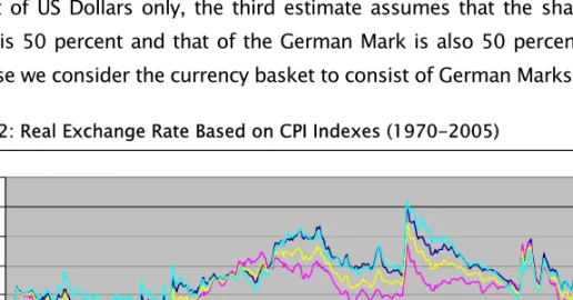
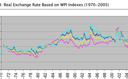
Figure 2 shows the time path of four different estimates of the RER based on CPI over the period 1970-2005. On the other hand, Figure 3 shows the time path of the four estimates of RER based on the approach of Sekkat and Varoudakis (2000). In Figure 3, the first estimate assumes that the currency basket consists of the currencies of a large number of countries with weights shown in Table 1. The second estimate considers the currency basket to consist of US Dollars only, the third estimate assumes that the share of US Dollar is 50 percent and that of the German Mark is also 50 percent. In the last case we consider the currency basket to consist of German Marks only.

Figure 2: Real Exchange Rate Based on CPI Indexes (1970-2005)

0 50 100 150 200 250 300 350 Jan-70 Jan-72 Jan-74 Jan-76 Jan-78 Jan-80 Jan-82 Jan-84 Jan-86 Jan-88 Jan-90 Jan-92 Jan-94 Jan-96 Jan-98 Jan-00 Jan-02 Jan-04 Zanello $ 0.5 $+0.5 DM DM

(8)

[\]Q ₁₆₂ _{JITD, Spring 2007}

Figure 3: Real Exchange Rate Based on WPI Indexes (1970-2005)

0 50 100 150 200 250 300 350 Ja n-70 Ja n-72 Ja n-74 Ja n-76 Ja n-78 Ja n-80 Ja n-82 Ja n-84 Ja n-86 Ja n-88 Ja n-90 Ja n-92 Ja n-94 Ja n-96 Ja n-98 Ja n-00 Ja n-02 Ja n-04 Zanello $ 0.5 DM+0.5 $ DM

Source : The authors

Figures 2 and 3 reveal that there are five episodes of RER developments during the period 1970-2005. In mid-1970, when Turkey faced a foreign exchange crisis, the RER was devalued by 65.78 percent. Thereafter the RER started to appreciate. After the foreign exchange crisis of late 1970’s, the RER depreciated sharply with the stabilization measures of 1980. It kept depreciating until 1988 and then started to appreciate again. Appreciation of the RER carried on until 1994 when the country was faced with another currency crisis. In 1994 the RER depreciated sharply but after a while RER started to appreciate again from April 1994 to February 2001 when the country was faced with the currency crisis of 2001. After the sharp depreciation of the RER during February 2001 to April 2001, the RER started to appreciate, with the appreciation accelerating after November 2001.

To emphasize the extent of annual inflation and rate of depreciation of the nominal exchange rate, we show in Figure 4 the time path of inflation and rate of depreciation of the TL/$ exchange rate, as the growth of CPI compared to its 12 month period lag value and as the

(9)

growth rate of the TL/$ exchange rate compared to its 12 month period lag value, respectively, on a monthly basis. The figure reveals that the annual rate of depreciation of the TL/$ exchange rate has exceeded the annual rate of domestic inflation during the crisis periods of 1970, 1980, 1994, 2001 and also during the period February 1980 – December 1984 when the government was deliberately pursuing a policy of RER depreciation. On the other hand, the rate of inflation has exceeded the rate of depreciation of the TL/$ exchange rate during the remaining periods, leading to an appreciation of the RER.

Figure 4: Annual CPI Inflation and Annual Rate of Devaluation of the Exchange Rate (1970-2005)

Source : The authors

We next turn to consideration of the foreign exchange regime followed by Turkey during the period 1970-2005. The IMF in its “Annual Report on Exchange Arrangements and Exchange Restrictions” classified the exchange rate policies based on information provided by the member countries. During 1970s the IMF indicated whether the country applied par (fixed) values or not. During 1974-82 it further reported whether the exchange rate was maintained within relatively narrow margins in terms

-50 0 50 100 150 200 250 300 Jan-70 Jan-72 Jan-74 Jan-76 Jan-78 Jan-80 Jan-82 Jan-84 Jan-86 Jan-88 Jan-90 Jan-92 Jan-94 Jan-96 Jan-98 Jan-00 Jan-02 Jan-04

(10)

[\]Q ₁₆₄ _{JITD, Spring 2007}

of the U.S. dollar, British sterling, French franc, South African rand or Spanish peseta, a group of currencies, or a composite of currencies. Finally, during 1970-82 the IMF also emphasized whether the country applied special rates for some or all of capital transactions, import rate different from export rate, more than one rate for imports, and finally whether more than one rate was applied for exports. After 1983 the number of classification categories was expanded to three. The three-bucket classification that prevailed through most of the 1980’s and 1990’s consisted of (i) pegged regimes, (ii) regimes with limited flexibility, and (iii) more flexible arrangements. The first broad regime group consists of two sub-groups, i.e. single currency pegs and composite currency pegs. The second group has been used to classify the European countries (prior to the monetary union) with exchange rate arrangements vis-à-vis one another (i.e. the Snake, the Exchange Rate Mechanism, etc.) and the Gulf countries. The third bucket includes two sub-groups, i.e. managed floats, either according to a set of indicators or in a country-specific way, and independent floats. In this classification the exchange rate arrangement (i) refers to fixed, (ii) to intermediate and (iii) to flexible regimes. However, the classification had two major shortcomings. First, it failed to capture differences between what the countries claimed to be doing and what they were actually doing. Second, by lumping rigid forms of pegs together with softer pegs it failed to acknowledge the different degree of monetary autonomy afforded by each regime. To address these shortcomings, in 1999 the IMF adopted a new classification scheme based on still de facto policies. The new scheme allows for eight different categories ranging from the adoption of a foreign currency as legal tender to free floats.2

2_{The eight regimes are: (I) dollarization and euroization, (II) currency board, (III)} conventional fixed pegs, (IV) horizontal bands, (V) crawling pegs, (VI) crawling bands, (VII) managed float with no preannounced path for the exchange rate, and (VIII) independent float. Under “conventional fixed pegs” the currency is pegged to another currency or currency basket within a band of at most +/- 1 percent. While “horizontal bands” refer to pegs with bands larger than +/- 1 percent, “crawling pegs” refer to pegs with central parity periodically adjusted in fixed amounts at a pre-announced rate or in response to changes in selected quantitative indicators. “Crawling bands” refer to crawling pegs combined with bands larger than +/- 1 percent. While “managed float with no preannounced path for the exchange rate” refers to a regime with active

(11)

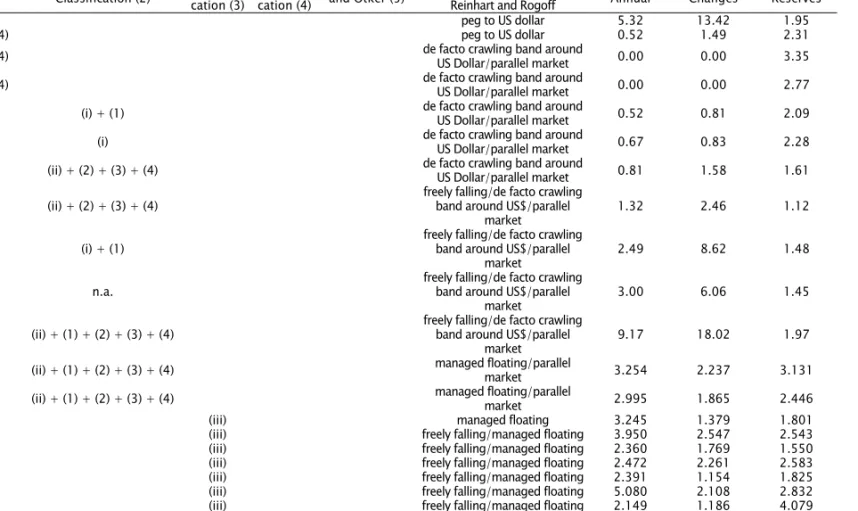
Table 2, in columns 1-4, shows the evolution of the Turkish exchange rate regime according to the IMF’s “Exchange Arrangements and Exchange Restrictions”. The table reveals that Turkey applied a par exchange rate regime during 1970-73, that the exchange rate was maintained within a relatively narrow margin during 1974-75, and that the exchange rate was not maintained within a narrow margin during 1976-82. According to the IMF, Turkey applied special rates for some or all capital transactions during 1970 and 1974. During 1971-73 Turkey applied import rates different from export rates, and more than one rate for exports, and during 1976-77 it applied, in addition, more than one rate for imports. During the 1980-82 period Turkey applied special rates for some or all capital transactions, import rates different from export rates, and more than one rate for imports and exports. After 1983 Turkey was classified as having “more flexible arrangements”. Later during 1996-97 it was classified as having a ‘managed floating’, during 1998-99 a ‘crawling peg’ and during 2000-05 an ‘independently floating’.

interventions without precommitment to a preannounced target or path for the exchange rate, the “independent float” regime refers to market-determined exchange rate with monetary policy independent of exchange rate policy. This classification treats exchange arrangements II, III, and I as fixed regimes, IV, V, and VI as intermediate regimes, and VII and VIII as flexible regimes.

(12)

Table 2: Exchange Rate Regimes

Volatility of Volatility of

Classification Exchange Exchange

IMF IMF IMF IMF of Babula Rates Rate Volatility of Classification ₍₁₎ Classification (2) _{cation (3)}Classifi- _{cation (4) and Otker (5)}Classifi- _{Reinhart and Rogoff}Classification of Annual Changes Reserves

1970 (i) + (1) peg to US dollar 5.32 13.42 1.95

1971 (i) + (2) + (4) peg to US dollar 0.52 1.49 2.31 1972 (i) + (2) + (4) de facto crawling band around _{US Dollar/parallel market} 0.00 0.00 3.35 1973 (i) + (2) + (4) de facto crawling band around _{US Dollar/parallel market} 0.00 0.00 2.77 1974 (i) + (1) de facto crawling band around _{US Dollar/parallel market} 0.52 0.81 2.09 1975 (i) de facto crawling band around _{US Dollar/parallel market} 0.67 0.83 2.28 1976 (ii) + (2) + (3) + (4) de facto crawling band around _{US Dollar/parallel market} 0.81 1.58 1.61 1977 (ii) + (2) + (3) + (4) freely falling/de facto crawling band around US$/parallel

market 1.32 2.46 1.12 1978 (i) + (1) freely falling/de facto crawling band around US$/parallel

market 2.49 8.62 1.48 1979 n.a. freely falling/de facto crawling band around US$/parallel

market 3.00 6.06 1.45 1980 (ii) + (1) + (2) + (3) + (4) freely falling/de facto crawling band around US$/parallel

market 9.17 18.02 1.97 1981 (ii) + (1) + (2) + (3) + (4) managed floating/parallel _market 3.254 2.237 3.131 1982 (ii) + (1) + (2) + (3) + (4) managed floating/parallel _market 2.995 1.865 2.446

1983 (iii) managed floating 3.245 1.379 1.801

1984 (iii) freely falling/managed floating 3.950 2.547 2.543 1985 (iii) freely falling/managed floating 2.360 1.769 1.550 1986 (iii) freely falling/managed floating 2.472 2.261 2.583 1987 (iii) freely falling/managed floating 2.391 1.154 1.825 1988 (iii) freely falling/managed floating 5.080 2.108 2.832 1989 (iii) freely falling/managed floating 2.149 1.186 4.079 1990 (iii) 9 freely falling/managed floating 1.834 0.978 2.816 1991 (iii) 9 freely falling/managed floating 4.854 2.929 4.688

(13)

Volatility of Volatility of Classification Exchange Exchange

IMF IMF IMF IMF of Babula Rates Rate Volatility of Classification ₍₁₎ Classification (2) _{cation (3)}Classifi- _{cation (4) and Otker (5)}Classifi- _{Reinhart and Rogoff}Classification of Annual Changes Reserves

1992 (iii) 9 freely falling/managed floating 4.296 2.142 4.776 1993 (iii) 9 freely falling/managed floating 4.433 1.579 3.553 1994 (iii) 7 freely falling/managed floating 10.770 15.141 8.115 1995 (iii) 9 freely falling/managed floating 3.579 2.515 14.266 1996 (iii) 9 freely falling/managed floating 5.222 1.245 8.618 1997 (iii) 9 freely falling/managed floating 5.538 0.944 8.913 1998 (iii) 7 crawling band around _{DM/freely falling} 3.659 1.812 12.500 1999 IV 7 crawling band around _{Euro/freely falling} 4.618 1.373 5.658 2000 IV 7 crawling band around _{Euro/freely falling} 2.323 1.102 8.480 2001 VIII 13 freely falling/freely floating 9.773 8.080 13.553

2002 VIII 3.247 3.310 7.190 2003 VIII 3.10 2.03 10.08 2004 VIII 3.00 2.90 3.77 2005 VIII 1.37 1.32 7.57 3.426 3.311 4.714 Notes:

1. The two regimes are (i) par (fixed), and (ii) not par. (1) indicates that special rates are applied for some or all capital transactions, (2) import rates are different from export rates, (3) more than one rate for imports, and (4) more than one rate for exports.

2. The two regimes are (i) exchange rate maintained within relatively narrow margin, and (ii) exchange rate not maintained within relatively narrow margins. (1) indicates that special rates are applied for some or all capital transactions, (2) import rates are different from export rates, (3) more than one rate for imports and (4) more than one rate for exports.

3. The three regimes are: (i) pegged regimes, (ii) regimes with limited flexibility, and (iii) more flexible arrangements

4. The eight regimes are: (I) dollarization and euroization, (II) currency board, (III) conventional fixed pegs, (IV) horizontal bands, (V) crawling pegs, (VI) crawling bands, (VII) managed floats with no preannounced path for the exchange rate, and (VIII) independent float path for the exchange rate, and (VIII) independent float

5. The thirteen regimes of Babula and Otker-Robe are: (1) formal dollarization and euroization, (2) currency union, (3) currency board arrangements, (4) conventional fixed pegs vis-à-vis single currency, (5) conventional fixed pegs vis-à-vis a basket of currencies, (6) horizontal bands, (7) forward looking crawling pegs, (8) backward looking crawling pegs, (9) forward looking crawling bands, (10) backward looking crawling bands, (11) tightly managed floats, (12) other managed floats with no predetermined exchange rate path, and (13) independently floating.

(14)

[\]Q ₁₆₈ _{JITD, Spring 2007}

On the other hand, while Babula and Otker-Robe (2002) distinguish

between 13 regimes3_{, Reinhart and Rogoff (2002) distinguish between 15}

regimes.4_{Table 2 in column 5 reports the exchange regimes followed by}

Turkey according to the classification of Babula and Otker-Robe. The table shows that Turkey during the 1990s under high capital mobility has abandoned the intermediate regimes of “forward-looking crawling bands” and “forward-looking crawling pegs” and moved towards a regime of free floats. The Turkish exchange regime, according to the classification of Reinhart and Rogoff (2002), is reported in column 6 of Table 2. This classification reveals that Turkey during 1980-82 had multiple exchange rates and also had active parallel (black) rates. Furthermore, annual inflation rate in Turkey was running above 40 percent during 1980 and during 1984-2001, which have been classified by Reinhart and Rogoff as ‘freely falling’.

We supplement the information provided in Table 2 columns 1-4 with the following additional measures: (i) “volatility of exchange rates” defined as the average of absolute monthly percentage changes in the

3 _{These regimes are: (1) formal dollarization and euroization, (2) currency union, (3)} currency board arrangements, (4) conventional fixed pegs vis-à-vis single currency, (5) conventional fixed pegs vis-à-vis a basket of currencies, (6) horizontal bands, (7) looking crawling pegs, (8) backward-looking crawling pegs, (9) forward-looking crawling bands, (10) backward-forward-looking crawling bands, (11) tightly managed floats, (12) other managed floats with no predetermined exchange rate path, and (13) independently floating. The crawl is viewed as “backward-looking” when the crawl aims to passively accommodate e.g. past inflation differentials under a real exchange rate rule, and as “forward-looking” when the exchange rate is adjusted at a preannounced fixed rate and/or set below projected inflation differentials, typically when the exchange rate is envisaged to have an anchor role. Under “tightly managed floats” interventions take the form of very tight monitoring that generally results in stable exchange rates without having a clear exchange rate path, so as to permit the authorities an extra degree of flexibility in deciding the tactics to achieve a desired path. Under “other managed floats with no predetermined exchange rate path” exchange rate is influenced in a more ad hoc fashion. The classification of Babula and Otker-Robe treats exchange arrangements 1, 2, and 3 as hard peg regimes, 4-11 as intermediate regimes, and 12 and 13 as floating regimes.

4_{The regimes are: (1) no separate legal tender, (2) pre announced peg or currency board} arrangement, (3) pre announced horizontal band that is narrower than or equal to +/- 2 percent, (4) de facto peg, (e) preannounced crawling peg, (5) preannounced crawling band that is narrower than or equal to +/- 2 percent, (6) de facto crawling peg, (7) de facto crawling band that is narrower than or equal to +/- 2 percent, (8) preannounced crawling band that is wider than or equal to +/- 2 percent, (9) de facto crawling band that is narrower than or equal to +/- 5 percent, (10) moving band that is narrower than or equal to +/- 2 percent, (11) managed floating, (12) freely floating, (13) freely falling, and (14) hyperfloats.

(15)

nominal exchange rate during a year, (ii) “volatility of exchange rate changes” defined as the standard deviation of the monthly percentage changes in the nominal exchange rate during a year, and (iii) “volatility of reserves” defined as the average of absolute monthly changes in the non-gold reserves, normalized by the reserve money in the previous month. We note that fixed regimes have low values for “volatility of exchange rates”, low values for “volatility of exchange rate changes” and high values for “volatility of reserves”. On the other hand, flexible regimes combine high values for “volatility of exchange rates” and “volatility of exchange rate changes” with low values for “volatility of reserves”.

The estimated values of volatility of exchange rates, volatility of exchange rate changes and volatility of reserves for Turkey reported in columns 7-9 in Table 2 for 1970-2005 reveal that the volatility of exchange rates, volatility of exchange rate changes, and volatility of reserves have been low during the 1970s. Furthermore, volatility of exchange rates and volatility of exchange rate changes during 1981-1990 and during 2000 have been relatively low, and during the period 1980-1988 when Turkey tried to achieve annual RER devaluation of about 6 percent, the volatility of reserves has been rather low. On the other hand, during 2000 when Turkey followed a semi currency board arrangement the volatility of reserves has been relatively high.

The volatility of reserves started to increase after the liberalization of international capital movements in 1989. As the exchange rate became more and more determined by the market, the volatility of exchange rates and volatility of reserves increased considerably during the periods 1991-1993 and also during 1995-2001. During the crises periods of 1994 and 2001, the values for all three measures increased enormously. During the period 2002-2005 the country has experienced relatively high values of volatility of reserves, but relatively low values of volatility of exchange rates.

(16)

[\]Q ₁₇₀ _{JITD, Spring 2007}

III. PRICE EFFECTS IN TURKISH FOREIGN TRADE

From economic theory we know that the current account balance improves with depreciation of the RER, worsens with increases in domestic absorption, and improves with increases in foreign absorption. To determine these relations empirically, we consider the imperfect substitutes model of international trade, the key underlying assumption of which is that neither imports nor exports are perfect substitutes for domestic goods. Import (export) demand and supply are modeled as functions of the relative price of imports (exports) and of aggregate demand for goods and services.

The Model

The quantity of imported goods demanded is assumed to depend on real domestic aggregate demand and the real exchange rate:

Md_{= M}d_{(π, AD)}

where Md_{is the quantity of foreign goods imported, AD is the level of}

real domestic aggregate demand measured at constant prices, and π = RER (1 + t). Here t is the ad valorem average tariff rate on imports. The demand for exports (foreign imports) depends on real foreign aggregate demand AD* and foreign relative price of imports π* by the rest of the world:

Md*_{= M}d*_{(π*, AD*)}

where Md*_{is the quantity of exports, π* = (p}_x_{/ E p}_f_{) is the relative price of}

imports abroad. Here px is the price of exportables by the home country

measured in terms of domestic currency, and pf is the foreign price of

commodities produced by the rest of the world measured in terms of foreign currency.

We assume that the supply schedules of importables are perfectly elastic. On the other hand, the supply of exportables in the home country is

(17)

assumed to depend on the price of exportables px, relative to the home

price p of goods produced by the home country, measured in terms of domestic currency and and real income y in the country:

Xs_{= X}s_(p_x_{/p , y)}

where Xs_{is the supply of home country exportables and y denotes the}

real GDP. Here, exports are assumed to rise as real income serving the purpose of an index of productive capacity of the country rises. Imposing the equilibrium condition in the market for exportables

Md*_{= X}s_,

and expressing all relations in natural logarithms we get

(1) ln M = α0 – α1 ln [RER (1 + t)] + α2 ln AD

(2) ln Md*₌_β₀_-_β₁_{ln (p}_x_{/E p}_f_{) +}_β₂_{ln AD*}

(3) ln Xs₌_γ₀₊_γ₁_{ln (p}_x_{/p) +}_γ₂_{ln y}

(4) ln Md*₌_{ln X}s

Solving equations (2) – (4) for exports we obtain

(5) ln X = a0 + a1 ln RER + a2 ln AD* + a3 ln y

where RER = (E pf/p), a1 > 0, a2 > 0 and the sign of a3 is indeterminate.5

Data Sources

We now consider the annual data for the period 1970-2005. Data on Turkish GDP at constant prices, on exports and imports of goods at current prices measured in US dollars, and on aggregate domestic demand defined as the sum of consumption, plus investment plus government expenditures at constant prices, have been obtained from

5_{The literature on trade equations is vast. Goldstein and Khan (1985) provide excellent} discussion.

(18)

[\]Q ₁₇₂ _{JITD, Spring 2007}

the State Planning Organization. Tariff revenue figures excluding the VAT payments on imported commodities at current prices were obtained from the website of the Ministry of Finance. Annual data on foreign aggregate demand, defined as the weighted sum of consumption plus investment plus government expenditures at constant prices of various OECD

countries, have again been obtained from the OECD.6_{Export and import}

price indexes of goods on a monthly basis were obtained from Central Bank publications and State Institute of Statistics. Finally, the RER data were obtained on a monthly basis following the method described above. The import and export values have been converted to real imports and exports using the export and import price indexes. In the estimation of import and export functions, we use real exports and real imports measured in terms of millions of 1987 US dollars. When estimating the import function we use RER data adjusted for the tariff rates as shown in equation (1).

Empirical Evidence

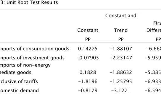
In order to observe the equilibrium relationship, we estimate the long-term stable relationship for exports and imports using their basic determinants. We adopted Johansen’s cointegration estimation method to identify the long-term relationship for these variables. Before going into the details of estimation, we performed heteroscedastic robust and Phillips and Perron (PP) unit root tests for the variables of interest. The test results are tabulated in Table 3. Test statistics cannot reject the presence of unit roots in levels for all the series considered when we included both constant, and constant and time trends. However, we can reject the null of the unit root with the intercept for the first differences of all the series. Therefore, we can safely assume that all the series considered are different stationary or I (1).

6_{The weight of Belgium is 4.47 percent, Canada 0.81 percent, France 11.07 percent,} Germany 26.66 percent, Italy 17.96 percent, Japan 4.94 percent, Netherlands 4.72 percent, Spain 3.8 percent, Switzerland 4.1 percent, United Kingdom 11 percent, and USA 10.47 percent.

(19)

Table 3: Unit Root Test Results

Constant and

Constant Trend

First Difference

PP PP PP

Real imports of consumption goods 0.14275 -1.88107 -6.6606** Real imports of investment goods -0.07905 -2.23147 -5.95951** Real imports of non-energy

intermediate goods 0.1828 -1.88632 -5.88581**

RER inclusive of tariffs -1.8196 -1.25795 -6.93367**

Real domestic demand -0.8179 -3.1271 -6.59466**

Real exports -1.30172 -2.4237 -6.10947**

RER -1.94938 -1.27677 -7.10945**

Real foreign demand -1.14475 -2.69017 -3.99087**

Note: ** indicates the level of significance at the 1 percent level and * indicates the level of significance at the 5 percent level.

The estimated import demand schedules are presented in Table 4. During the estimation we first separate total imports into energy and non-energy imports. Next, we split non-energy imports into imports of consumption goods, imports of investment goods, and imports of non-energy intermediate goods. We note that for practical purposes, non-energy imports depend on the price of oil rather than the RER. Splitting non-energy imports into consumption, investment and non-non-energy intermediate goods is relevant since the RER elasticity of consumption goods, investment goods, and non-energy intermediate goods are quite different, and since there may be an increase in imports of intermediate goods over time reflecting a structural shift in the export pattern towards assembly-driven operations as a result of closer integration into international production networks. The results show that the RER elasticity of imports of consumption goods, investment goods and non-energy intermediate goods, in case a CPI-based measure of the RER obtained using the method of Zanello and Desruelle (1997) is used, are

(20)

[\]Q ₁₇₄ _{JITD, Spring 2007}

2.1843, 0.874121 and 1.0376 respectively.7_{Similarly domestic demand}

elasticity of imports of consumption goods, investment goods, and non-energy intermediate goods are 3.2217, 2.11076 and 2.3039 respectively. The figures reveal high susceptibility of import flows to aggregate domestic demand.

Table 4: Import Functions

Logarithm of Logarithm of

CPI based real

Dependent RER inclusive domestic

variable Constant of tariffs demand

Real imports of -19.72558 -2.18433 3.22173 consumption goods (-5.5519) (-3.0060) (9.94611) Real imports of -12.55229 -0.874121 2.11076 investment goods (-7.104493) (-2.318562) (12.61209) Real imports of non-energy imports -12.47592 -1.03757 2.30387 of intermediate goods (-4.9575) (-1.9919) (11.0879)

Note: t-statistics are displayed in parenthesis.

The estimated export supply schedule is given in Table 5. The elasticity of exports with respect to foreign aggregate demand is estimated as 3.4085. On the other hand, price elasticity of exports, when the CPI-based measure of the RER obtained using the method of Zanello and Desruelle (1997), is measured as 0.3403.

7_{When deflating the export and import values measured in terms of current US Dollars by} the export and import price indexes we have used for the period 1970-1995, the price indexes published on a monthly basis by the Central Bank of Turkey, and for the period 1996-2005, the price indexes published by the State Institute of Statistics. The import values of investment goods have been deflated by the import price index of investment goods published by the Central Bank of Turkey over the period 1970-1995. All other import and export values have been deflated by the general price indexes respectively as obtained above.

(21)

Table 5: Export Function

Logarithm of Logarithm of

CPI based real

Dependent RER inclusive foreign

variable Constant of tariffs demand

Logarithm of -43.6101 0.3403 3.4085

real exports (-6.1369) (0.437) (5.4118)

Note : t-statistics are displayed in parenthesis.

We note that the Marshall-Lerner condition holds as the absolute values of estimated price elasticities for imports determined by the relationship

)

(

)

(

)

(

m

_ne ne inv inv con con im

η

=

+

and exports sum up to more than unity, where ηcon denotes the price

elasticity of imports of consumption goods, ηinv price elasticity of imports

of investment goods, ηne price elasticity of imports of non-energy

intermediate goods, mcon imports of consumption goods, minv imports of

investment goods, mne imports of non-energy intermediate goods, and

m total imports. We note that import price elasticity is ηim = 0.9676 and

that export price elasticity is ηex= 0.3403. The Marshall-Lerner condition

indicates that the trade balance improves following a real depreciation of the domestic currency.

IV. A FRAMEWORK FOR ASSESSING THE SUSTAINABILITY OF THE CURRENT ACCOUNT

Swan (1963), in a path-breaking paper taking productivity, the terms of trade, capital movements and other financial variables as given and assuming no special import restrictions imposed on balance of payments grounds, shows how employment and the balance of payments both depend on the level of spending and on the relative cost situation. In Figure 5 ‘real expenditure’ is the total domestic investment and consumption

(22)

[\]Q ₁₇₆ _{JITD, Spring 2007}

(private and public) at constant prices, called AD for short; and the ‘cost ratio’ is an index measuring competitive position of industries.

Figure 5: Swan Diagram

Source : Swan (1963)

Considering that for the cost ratio RER, we note that a given level of employment can be sustained with AD very low if RER is high enough, and vice versa. This is shown by Schedule A, where A2 refers to full

employment, A1 underemployment and A3 over-employment. Similarly a

given balance of payments requires a combination of low RER and low AD, or high RER and high AD. This is shown by Schedule B, where B2

stands for sustainable level of balance of payments deficit, B1 for a

relatively smaller deficit and B3 for a relatively larger deficit. Swan (1963)

points out that there are many A and B curves for different levels of employment and balance of payments.

Any combination of RER and AD along A2 gives the internal balance, and

any combination of B2 gives external balance. The intersection of these

two curves gives us the equilibrium values of RER and AD that will attain internal as well as external balance. The equilibrium value of the RER,

(23)

called the fundamental equilibrium exchange rate (FEER), is thus a normative one, and it is characterized by Williamson (1994) as the equilibrium exchange rate that would be consistent with ‘ideal economic conditions’.

Although the determination of the internal balance relation A2 is rather

straightforward, the determination of external balance B2 depends on the

way that the sustainable level of current account is defined. To attack the problem of determination of sustainable level of current account, we consider the simple accounting methodology developed by Milesi-Ferretti and Razin (1996), which makes use of the balance of payments

relation written as $

−

*

₁

+

−

₁

=

0

− − t t t t t

i

D

FDI

D

TB

where TB$_denotes

the non-interest current account, i* the foreign rate of interest, D the stock of foreign debt, and FDI the foreign direct investment inflow. Note that

(

TB

t$

−

i

*

D

t−1

)

=

Current

Account

t and

t t

t

D

Capital

Account

FDI

+

−

₋

)

=

(

₁ _{, where all variables are measured}

in terms of foreign currency. Writing the non-interest current account explicitly by splitting total imports into energy and non-energy imports and considering the EU grants we have:

TB$_{= Exports – Energy Imports – Non-Energy Imports + EU Grants +} Other

where all variables are measured in terms of foreign currency, and ‘Other’ stands for Current Account - Exports + Energy Imports + Non-Energy Imports + i* Dt -1 - EU Grants.8

Next we define the non-energy and non-interest current account

surplus, NETB = (Exports – Non-Energy Imports + Other). If

t t t t t

y

p

D

E

d

=

8_{Here we assume that EU grants are in the form of current transfers. If EU grants would} be in the form of capital transfers, they would be shown not in the current account but in the capital account of the balance of payments. Since this is purely a matter of definition, for our purposes it is not of importance whether EU grants are shown under current account or capital account of the balance of payments.

(24)

[\]Q ₁₇₈ _{JITD, Spring 2007}

is the foreign debt to GDP ratio; ne

t t t t t

y

p

NETB

E

tb

$

=

the non-interest non

energy current account surplus in proportion to GDP; energy = (E x Energy Imports / py) the energy import bill to GDP ratio; eugrants = (E x EU Grants / py) the EU grants to GDP ratio; and

t t t t t

y

p

E

FDI

fdi

=

the FDI to

GDP ratio, the equation determining the time path of dt which also stands for the economy’s intertemporal financing constraint can be written as: (6) t t t t t t t t

t

d

energy

eugrants

fdi

g

r

netb

d

+

−

+

−

=

* ₋₁

)

1

(

)

1

(

)

1

(

η

, where * t

r

denotes the foreign real rate of interest and η_{t the rate of}

depreciation of the RER. The equation reveals that the external debt to GDP ratio decreases with increases in the non-interest, non-energy current account surplus in proportion to GDP netb, EU grants to GDP ratio eugrants, the FDI to GDP ratio fdi, and the growth rate of GDP g. By contrast, the debt to GDP ratio increases with increases in the foreign real interest rate r*, rate of depreciation of the RER η_{, and energy import}

bill to GDP ratio energy.

Following the approach of von Hagen and Harden (1994), we solve the

economy’s intertemporal financing constraint forward for n periods and

obtain: (7)

∑

= + +

+

Γ

=

n i ti t i t n t n t t t

d

A

d

1 , ,

δ

_where

∏

=

+

=

k i i i i k t

r

g

1 * ,

)

1

(

)

1

(

1

η

δ

_and t t t t

t

netb

fdi

eugrants

energy

A

=

+

−

. Here,

δ

t,k can be interpreted as

the ‘k-periods ahead’ discount factor used to calculate the present value of assets and liabilities in period t + k for period t, and

Γ

t

x

t+k denotes the period t expectation of the variable x in period t + k. The economy’s intertemporal financing constraint indicates that, when intertemporal solvency holds (so that dt+n is finite), current debt-to-GDP ratio equals the

(25)

expected discounted present value of foreign debt outstanding in period t+n relative to GDP, plus the sum of all discounted At s between period t and period t + n.

To translate the intertemporal budget constraint into a practically more relevant requirement for debt sustainability, we consider the budget constraint for a limited period of time n* and add the sustainability condition that the discounted debt/GDP ratio at the end of period t+n*, discounted dt+n* should not exceed the debt/GDP ratio at time t, dt. Thus,

current account is not sustainable if:

(8)

S

(

n

*)

=

d

_t

−

Γ

_t

δ

_t_,_n

d

_t₊_n

<

0

.9

but this sustainability condition, while useful, is not easy to assess in practice. Even under initial negative At values over the next few years, the

current account can be said to be sustainable if during the latter periods large positive non-interest non-energy current account to GDP, EU grants to GDP, FDI to GDP and relatively low values of energy import bill-to-GDP ratios are assumed. The analysis thus depends on the assumptions one makes about the evolution of At+n over time.

V. SCENARIOS FOR THE SUSTAINABILITY OF THE CURRENT ACCOUNT In the exercise conducted below we introduce the following assumptions:

• _{We assume that n* = 10, and assume in the base case the continuation}

of the present policies into the future. In particular we assume that the value of netb2005+i for i = 1, . . . , 10 will remain unchanged at its initial value of netb2005 = 0.2845 percent.

9_{The formulation of the sustainability problem through the difference equation (6)} assumes that FDI is a surer and safer form of external financing. Thus the analysis is the paper assumes that current account deficits financed mainly by FDI inflows does not lead to problems of sustainability of current account, but if FDI takes the form of purchases of stocks and if these shares can be liquidated easily in domestic markets, then it is possible to take the money out of the country as in other forms of investment. In those cases FDI makes no difference and there is no reason to separate FDI flows in the difference equation (6). Under these conditions, sustainability of the current account will require higher rates of depreciation of the RER than those obtained in our analysis given in section 4.

(26)

[\]Q ₁₈₀ _{JITD, Spring 2007}

• _{In the case of energy products, we note that the average price of oil}

($/barrel) has increased from $54.45 in 2005 to $64.34 in 2006, and

that the price of Russian natural gas (US$/1000 m3_{) from $212.94 in}

2005 to $290.40 in 2006. Concentrating in the following on oil imports only we assume under the base case that the price of oil (US$/barrel) will decrease to $58.4 in 2007 and to $50 thereafter. Thus, given

energy2005= 5.39 percent we have energy2006 = 6.37 percent, energy2007

= 5.79 and energy2005+i = 4.95 for i = 3,..,10.

• _{Regarding EU grants, we assume in the base case that EU grants amount}

to 300 million Euros in 2005, 500 million Euros in 2006, 550 million Euros during 2007-2009, 700 million during 2010-2013 and 2 billion Euros during 2014-2015.10

• _{Regarding the growth rate of real income, we note that the average}

value of the growth rate of real GDP amounted to 4.08 per cent during 1980-1989 and to 4.3 percent during 1990-2005. The 2005 ‘Pre-Accession Economic Programme’ published by the State Planning Organization at the end of 2005 foresees a growth rate of 5 percent over the next few years. The growth rate of real GDP in 2006 is expected to be around 6 percent. For the growth rate of GDP over the time period 2007 to 2015 we take the figure of 5 per cent in the base case, i.e. g2005+i = 0.05 for i = 2,.., 10.

• _{To determine the foreign interest rate, we use the yields on Eurobonds}

issued by the Turkish Treasury. The average rate of return on Turkish US dollar-denominated Eurobonds during the last few years amounted to 12.515 percent in 2002, 10.852 percent in 2003, 8.605 percent in 2004, 7.93 percent in 2005, and 7.13 percent during the first few months of 2006.11_{Considering the value of 7.93 and deflating it by}

expected US CPI inflation rate over the next few years, we obtain a figure of 5.91 percent for foreign real interest rate. In the following we

10 _{When converting the Euro values into US Dollar values we use the exchange rate where 1} Euro equals US$ 1.25.

11_{We would like to thank Tekin Cotuk of the Undersecretariat of the Treasury for providing} the data on Turkish Eurobonds.

(27)

take the figure of 6 percent for real foreign interest rate in the base case, i.e. r*2005+i = 0.06 for i = 1,.., 10.

• _{Next we consider the rate of depreciation of the RER. Although the}

CPI-based RER has appreciated over the period 2002-2005 at the annual rate of 7.53 percent, and the WPI-based RER at 7.66 percent, we abstract from further appreciation or depreciation of the RER under the base case due to the Balassa-Samuelson effect under the base case and assume that η_{2005+i = 0 for i = 1, . . . , 10.}12

• _{Concerning the FDI/GDP ratio, we note that while, during the period}

2002-2004 the average FDI/GDP ratio amounted to 0.76 percent, the ratio increased to 2.7 percent in 2005 as a result of privatizations and private sector mergers and acquisitions. On the other hand, the 2005 ‘Pre-Accession Economic Programme’ foresees FDI/GDP ratio of 1.367 percent over the next few years. Preliminary “best guess” estimates of FDI inflows for 2006 amount to $19 billion, and the forecasts are $14.2 billion for 2007, $8.5 billion in 2008, $8.2 billion in 2009 and $8 billion thereafter.

Next we consider a high-case scenario. Here we assume the price of energy products to revert to a lower level (temporary shock) starting from the fourth quarter of 2006.13_{Concentrating on the price of oil, we assume that}

the average price of oil (US$/barrel) will decrease from $62.33 in 2006 to $44.00 in 2007 and further to $41.50 thereafter. Furthermore we assume that the growth rate of real GDP will amount to 7 percent, and the foreign real interest rate will be 4 percent during the period 2007-2015. The assumptions introduced in the base and optimistic cases are summarized in Table 6.

12_{For a discussion of Balassa-Samuelson effect see Togan and Berument (2006). Note that} the current account is assumed to be independent of RER appreciation, driven by productivity growth.

13_{In the fourth quarter of 2006 the average price of oil (US$/barrel) is assumed to be} $56.42 under the base case and $48.50 under the optimistic scenario.

(28)

Table 6: Assumptions of the Base and Optimistic Cases

Annual FDI Balassa- Samuelson Oil Price Growth Rate of GDP Foreign Real Interest Rate Non-Interest Non-Energy Current Account A

EU grants Inflow Effect Base Optimistic Base Optimistic Base Optimistic -to-GDP _Ratio Base Optimistic Time Euros US$ billion (percent) $/barrel $/barrel (percent) (percent) (percent) (percent) (percent) (percent) (percent)

2006 500 million 19 0 64.34 62.33 6 6 6 6 2005 level -1.050 -0.852 2007 550 million 14.2 0 58.50 58.50 5 7 6 4 2005 level -1.870 -0.502 2008 550 million 8.5 0 50.00 41.50 5 7 6 4 2005 level -2.528 -1.766 2009 550 million 8.2 0 50.00 41.50 5 7 6 4 2005 level -2.696 -1.963 2010 700 million 8 0 50.00 41.50 5 7 6 4 2005 level -2.793 -2.087 2011 700 million 8 0 50.00 41.50 5 7 6 4 2005 level -2.882 -2.201 2012 700 million 8 0 50.00 41.50 5 7 6 4 2005 level -2.967 -2.307 2013 700 million 8 0 50.00 41.50 5 7 6 4 2005 level -3.048 -2.407 2014 2 billion 8 0 50.00 41.50 5 7 6 4 2005 level -2.843 -2.257 2015 2 billion 8 0 50.00 41.50 5 7 6 4 2005 level -2.930 -2.359

(29)

Regarding foreign debt, we note that we have two sets of data. The first set is produced by the Turkish Treasury. With this data, the debt-to-GDP ratio in 2005 equals 46.9 percent. A second set of data which we use in our analysis is provided by Lane and Milesi-Ferreti (2006) for the period

1970-2004.14_{The authors define the net foreign assets as foreign assets}

minus foreign liabilities, and estimate the figures for 145 countries. Foreign assets are defined as the sum of portfolio equity assets, FDI assets, debt assets, and total reserves minus gold. Similarly foreign liabilities are defined as the sum of portfolio equity liabilities, FDI liabilities, and debt liabilities. In the following, we adjust Lane and Milesi-Ferreti’s (2006) data, so that the estimates become consistent with the relation Dt = Dt-1 - Current Accountt - FDIt used in our analysis, where Dt denotes the net foreign liabilities defined as foreign liabilities

minus foreign assets. We consider Lane and Milesi-Ferreti’s foreign asset figure, but define foreign liabilities as the sum of portfolio equity liabilities and debt liabilities. The debt-to-GDP ratio in 2005 using the adjusted Lane and Milesi-Ferreti’s figures turns out to be 35.57 percent.15

We then calculate the value of the debt-to-GDP ratio in 2015 using the difference equation (6) and then the value of the sustainability measure (8). When under the base case

A

t

=

netb

t

+

fdi

t

+

eugrants

t

−

energy

t for t = 2006, .., 2015 equals the values shown in Table 6, the current account in 2005 turns out to be unsustainable in the sense that the actual debt-to-GDP ratio in 2005 falls short of the expected discounted present value of foreign debt outstanding in period 2015 by 24.42 per cent. The sustainability of the current account requires that the value of the sustainability measure be increased so that it becomes zero or positive. This goal can be achieved through increases in non-energy

14_{The data set of Lane and Milesi-Ferreti (2006) is available via the Internet at} http://www.imf.org/ external/pubs/ft/wp/2006/data/wp0669.zip.

15_{We do not use the foreign debt figures of the Treasury as they are generally not} consistent with the relation Dt = Dt-1 - Current Accountt - FDItused in our analysis, where Dt denotes the net foreign liabilities defined as foreign liabilities minus foreign assets.

(30)

[\]Q ₁₈₄ _{JITD, Spring 2007}

non-interest current account to GDP ratio netb2005+i, EU grants to GDP

ratioeugrants2005+i , FDI to GDP ratio fdi2005+i , or through a decrease in

energy to GDP ratio energy2005+i during the period 2007-2015, or

through a combination of increases in both the non-energy non-interest current account to GDP, EU grants to GDP and FDI to GDP ratios, and a decrease in energy to GDP ratio over time. To achieve the minimal condition for external sustainability, Turkey has to increase the value of At during each period from 2006 to 2015.

Suppose first that fdi2005+i , energy2005+i and EU grants for i = 1, .., 10 amount to values shown in Table 6 under the base case. Economic theory tells us that non-energy, non-interest current account to GDP ratio net can be increased by decreasing the aggregate demand for domestic goods and services and/or by depreciating the RER. Decreasing the aggregate demand for goods and services would require that the country use contractionary policies. Overall, although adjustments are possible, little margin for further tightening of macroeconomic demand management policies may exist in the coming years in view of the high real interest rates and the large general government primary fiscal surplus—equivalent to 6.5 percent of GDP.

In the absence of adjustment in the underlying fundamentals for current account sustainability (FDI, energy bill, grants, domestic demand), changes in the exchange rate are the other possible adjustment mechanism for maintaining long-term sustainability of the current account. Depreciation of the RER increases exports and decreases imports via the direct RER effect considered in Tables 4 and 5, but depreciation of the RER also contains the growth in domestic aggregate demand, and thus limits import growth and helps restore the sustainability of the current account through this more indirect channel. The estimated aggregate demand function shown in Table 7 reveals that depreciation of the RER reduces the aggregate demand, which in turn reduces imports through the aggregate demand effect shown in Table 4.

(31)

Table 7: Aggregate Demand Function

Logarithm of

CPI based Logarithm of

Dependent RER inclusive real

variable Constant of tariffs GDP

Logarithm of

Domestic Aggregate 0.6030 -0.1190 0.9964

Demand (1.5993) (-2.1228) (40.9769)

Note: t-statistics are displayed in parenthesis.

To determine the extent of depreciation in the RER required, all else being equal, for achieving current account sustainability in the baseline scenario, we consider the effect of percentage change in RER on non-interest, non-energy current account to GDP ratio, given by

)

/

(

RER

d

GDP

NETB

d

=

θ

_{, which can be expressed as:}

)

]

[

1

)

(

η

_exp

η

γ

ε

θ

m

RER

x

y

m

RER

_ne ne inv inv con con imp

−

+

=

,

where η_imp_andη_exp_{denote the import and export elasticities with respect}

to the RER, γcon is the elasticity of imports of consumption goods with

respect to aggregate demand, γinv is the elasticity of imports of

investment goods with respect toaggregate demand, γne is the elasticity

of imports of non-energy intermediate goods with respect to aggregate

demand, ε is the elasticity of aggregate demand with respect to RER, x is

the real exports, m is the real imports and y is the real GDP. From previous considerations, we know that export price elasticity is 0.34 and import price elasticity is 0.97. On the other hand, the elasticity of imports of consumption goods with respect to aggregate demand is 3.22, the elasticity of imports of investment goods with respect to aggregate demand is 2.11, and the elasticity of imports of non-energy intermediate goods with respect to aggregate demand is 2.30. Table 7 reports that the elasticity of aggregate demand with respect to

(32)

[\]Q ₁₈₆ _{JITD, Spring 2007}

RER is ε = -0.119. Since during 2005 the export-to-import ratio was

62.98 percent and import-to-GDP ratio was 26. 6 percent, we have θ₌

8.98. Thus, a reduction in the ratio of the non-energy, non-interest current account by 1 percentage point of GDP requires a depreciation of the RER by 8.98 per cent. Thus sustainability of the current account in the base case requires that the RER be depreciated by 22.87 per cent. The above results were derived from equation (6) for the value netb2005+i for i = 2,..,10 that would satisfy the sustainability condition S(10) = 0. The results show that netb2005+i for i = 2,..,10 has to be increased by 2.55 percent. Solving the difference equation (6) for the value of debt-to-GDP ratio in 2015, with the values of energy2005+i , eugrants2005+i , and fdi2005+i of the base case for i = 1,..,10 shown in Table 6, and all other

parameters remaining at their base scenario values, we note that the debt to GDP ratio increases from its value of 35.57 per cent in 2005 to 38.74 per cent in 2015. This increase in debt-to-GDP ratio is thus perfectly compatible with the sustainability condition specified above, but note that the estimated value of the increase in debt-to-GDP ratio from 35.57 percent to 38.74 percent does not consider the effect of changes in RER on debt-to-GDP ratio. Since by definition

)

(

)

(

_* t t t t t t t t t

y

D

p

RER

y

p

D

E

d

=

,

we note that RER changes will affect the value of debt-to-GDP ratio, and that depreciation of the RER will lead to further increases in debt-to-GDP ratio. Hence, the results obtained above are downward-biased. They need to be corrected accordingly. In particular under the base case when RER depreciates by 22.87 percent, the debt-to-GDP ratio will not increase to 38.74 percent but rather to 47.6 percent.

The above considerations reveal that sustainability of the current account can be achieved with depreciation of the RER by 22.87 percent, but under relatively large increases in debt-to-GDP ratio from 35.57 percent

(33)

to 47.6 percent. An alternative specification of the sustainability condition requires that the ratio of the stock of net foreign liabilities-to-GDP, after say 10 years, taking account of the effect of RER changes on the debt-to-GDP ratio does not increase above its initial value attained during the time period 2005. Since this is a stronger condition than that of von Hagen and Harden, we note that attainment of sustainability requires now that the RER be depreciated by 33.2