Growth oriented adjustment programs : a statistical analysis

Trade Policy

Counitry Economics Department The World Bank

June 1990 WPS 426

Growth-Oriented

Ad justment Programs

A Statistical

Analysis

Riccardo Faini

Jaime de Melo

Abdel Senhadji-Semlali

and

Julie Stanton

There is no statistical evidence that growth was faster

-

or

slower

-

for countries that received adjustment loans. And

there are no signs of sustainable recovery through higher

invest-ment- at least through 1986.

Thc Policy. Rce.arch, and lixemi A AffAtrs ('rinip:v d. I c l'K !r.k Inh i dg atie, the findings of *ork in progrcss and to cnexurge the exchange of id as amorng II ank sLa!t and ,I ai' rtn k: desc>_wocrnt mn [hese papcrn carT) the names of the auLhor,, mrelw 'rl N ot r ,*.* and s : ' :.. .I. < .. tc.tg> I !rt;onn, -and ': .,rca * it. Lis ionn arc rhc auLhor' o*.n The.n sh nu i nno he jlatrh- lU- d nc Vi r..' m, It r l,. ,r I) ,.: rx, g.nf m a, k w ir fL, 7ncbcr e mnnres

Public Disclosure Authorized

Public Disclosure Authorized

Public Disclosure Authorized

Trade Pclicy

WPS 426

T hisppaper a- product of ltleTralde Polic) Di ision Counltr EconomicsDepartnmct-ispartofalarger

effort in PRE to analyze thc sustainabilitv oi structural adjustie nt programs. The paper is part of thc research project orn trade refonrm in structural adjustment loans (RPPG 675-32). Copies are available free from the World Bank, I81 Ili Strcet NW, Washington DC 2(033. Please contact Maria Ameal, room NI(-031, extension 37947 (33 pages '. ith tahbes).

What happened to cconiomic perrirmanic in 1Thc found that a higher current account developing countrics under oro( ih-oricniitd surplus and loAer inflation during 1978-81 were adjustmcnt programs sponsored i' tteC World associ;itcd

~

ith bcttcr investmcnt pertormancc Bank and thte INiF? d uring 19S2-S6. And that deterioration in the

external environment in 1982-86 was associated Analyzinjg data for a sample of 93 CoLuntriC S. ith lo er gro lh during thiat period.

Fai li, de M(elo, Senhadji-SelLikii, and St anton

compared the average values of cconomic Thic) also cxa;mincd the investmnclt-output indicators for 1982-86 with the corrcspondinei relationship lor 14 countries that received sizable values lr 1978-8 1. They control lcidlor the Lrow th-ori.rintedi adjustment loans -- estimatlingi

external environment and initial condition:%, antd the g-.ro( ii 10rConie because of lo, r a-t regate

al loA ced or policies that l ould 1 % c ha n v c,tment i u ndier adjustmenl

idopldt iI tlie CoultllieoS hIci Iated in

aidjUstlimCeIt. IlhC\ CoiK I Iiu' l;tat Sieil5 Oi SuStai nlble

ICC~\ I ! t h ron eh hi h r invcstientw Acre uno,

Thic toutilld o tati cal cx idenee tdeniit. l at Iax it throu ieh 19S6. 3ut Ltlhese results (or slok er) e,rox t lih ? 1 t C n t r1 I t hi I I a rIei I 'ri, d nt 'urprisi: ht ecausc considerable timeic

loans. nI ,1 a 1', iol or the b nefits of structural relfonn to

n at c n ll l/ e

Fh,k 'RI. Woiirking P'.q;><r A<1>x,>'!,I.i' i". _, .! Uq Ti ilt; i C i T 11 1 !!1; lIx i < %'i I R car 8;u , wi.d F .. i c rTl .i

A tI lr ( .1ic:< x A i k 5 > i, ,i 1 ti i T i 1 i < - t ci t1 irl,.!!g C"I Ce.tKi+' 11 it I)TOICrIIA11011S .u. 11!SS t11.u fUli'L

by

Riccardo Faini (Johns Hopkins University) Jaime de Melo (The World Bank and CEPR) Abdel Senhadji-Semlali (University of Pennsylvania)

and

Julie Stanton (University of Maryland)

Table of Contents

1. Introduction 1

2. External Environment and Adjustment Lending 2

3. An Implementable Model to Measure Effectiveness 6

of IMF-WB Programs

3.1 Alternative Approaches to Evaluating Adjustment 6 Programs

3.2 Implementation 8

4. Statistical Results 10

5. Sustainability of Adjustment: Output Loss Estimates 13 from Investment Cuts for a Group of Intensive

Adjustment Lending Recipients

6. Conclusions 20

Footnotes 23

References 24

Appendix 27

* We thank Bela Balassa, Ajay Chhibber, Patrick ConrJay, Vittorio Corbo, Peter Montiel, John Nash, and Dani Rodrik for helpful comments. Helpful comments were also received from seminars at Berkeley, Urbino, and at a conference on Adjustment Lending held at the World Bank. This paper is part of RPO 675-32.

1. Introduction

The decade of the 1980s will be remembered as one of unfulfilled

expectations for developing countries. Average per capita GDP growth fell

from 3.1 percent in the 1970s to 0.6 percent in the 1980s, and for many countries, private per capita consumption growth was negative. Adjustment lending programs supported by the International Monetary Fund (IMF) and the

World Bank (WB) were launched in response to the deteriorating external

environment. Restoring growth has remainei the focal concern of adjustment lending. Indeed, it is this greater emphasis on growth that disLinguishes the adjustment programs of the 1980s from their predecessors. The purpose of this paper is to assess statistically the extent to which adjustment programs supported by the IMF and the WB have restored growth. l/

The paper offers a fairly systematic evaluation of :MF-WB

supported adjustment programs. The evaluation relies on a large sample of countries (93) and controls for some of the statistical difficulties associated with measuring the effectiveness of adjustment programs. In

section 2, we review briefly the environment under which 1MF-'sB lendinlg

took place, the rationale for adjustment lending, and the distribution of adjustment loans through time. The methodology is described in section 3. The results of the statistical evaluation in section 4 suggest that, after controlling for external factors and for initial conditions, growth is not

higher in countries recipient of IMF-WB Fund , but that investment was

significantly lower than for non-recipient countries. This result leads us to examine further long-term growth prospects in section 5. There, for a

group of 15 countrie_ that received IMF-WB adjustment loans, we estimate a

simple growth model where capital is the only binding factor on output.

This model allows us to measure the approximate output loss incurred during

adjustment programs due to the combined reduction of private and public

investment. Conclusions follow in section 6.

2. External Environment and Adjustment Lending

The proximate causes of the worsening performance of developing

countries during the 1980s are well-known. For oil-importing countri!s,

the foreclosing of commercial credit and higher real interest rates on

co-mmercial _{borrowing came on top of the second oil price shock. Within}

this group of countries, exporters of primary commodities were further

adversely _{affected by declining prices for primary commodities as the}

dollar appreciated. For oil exporters, deterioration in the terms of trade

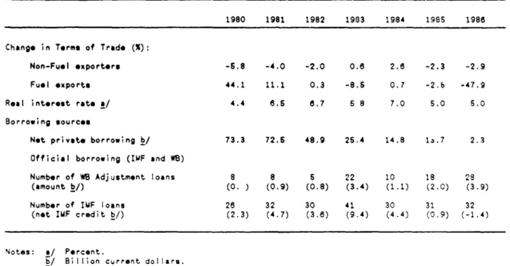
came later, but they were also adversely affected by the foreclosing of commercial funds. This adverse evolution of the external environment for developing countries is summarized in the top of table 1. Using these measures, in table 2 we provide a measure of the loss in purchasing power during 1982-6 due to the unfavourable environment of the 1980s. The loss is estimated at between 3.8 and 4.5 percentage points of average GDP during 1982-6.

As can be seen from the macroeconomic indicators in table 2, as a result of the deteriorating external environment, developing countries had difficulty in improving their current account position during the eighties and they increased substantially their external indebtedness. Also, table 2 indicates that the cut in expenditures that accompanied the adjustment to

Table 1: TERMS-OF-TRADE, REAL INTEREST RATES AND BORROWING SOURCES

1980 1981 1982 1903 1984 1955 1988

Change in Terms of Trade (%):

Non-Fuel exporters -5.8 -4.0 -2.0 0.8 2.6 -2.3 -2.9

Fuel exports 44.1 11.1 0.3 -8.6 0.7 -2.5 -47.9

Real interest rate a/ 4.4 6.5 8.7 5 8 7.0 5.0 5.0

Borrowing sources

Net private borrowing b/ 73.3 72.6 48.9 25.4 14.8 1a.7 2.3

Official borrowing (IMF and WS)

Number of WB Adjustment loans 8 8 5 22 10 18 28

(amount b/) (0. ) (0.9) (0.8) (3.4) (1.1) (2.0) (3.9)

Number of IMF loans 26 32 30 41 30 31 32

(net IMF credit b/) (2.3) (4.7) (3.8) (9.4) (4.4) (0.9) (-1.4)

Notes: a/ Percent.

b/ Biion current dollars.

the more unfavourable external environment involved a reduction in the share of investment expenditures in GDP.

It is in response to these balance of payments difficulties that adjustment lending was initiated by the WB (SALs and SECALs) and that adjustment programs by the IMF (EFFs and standby arrangements) were intensified. 2/ Participation by these international agencies was intended to assist recipient countries in designing packages that would help achieve two objectives. First, the packages would help stabilize the economy by adopting measures to restore a sustainable balance between aggregate demand and aggregate supply. Second, the packages would help production in the

short-run, especially in tradabl's because of the need to generate

increased net foreign exchanze earnings to meet 'arger ;ert service

payments. In our companion paper (Faini, et. al. 1989), *e show that tnis objective was met by a significantly larger real exchange rate qevauao

for countries that participated in adjustment programs sup.port- c by the M!F

and the World Bank. As emphasized by Corbo et as. L9 7\ e -.o:e

emphasis of adjustment programs in the eighties waS he e,.as s

restoring long-run growth, henrce the label g:uw-.:n: I

programs.

The distributicn of ad'ustment loans t3nu ..-. : ;e -.

by the WB are given at the bottom of table 1. The table ;-.wi -he •hRr

drop in the availability of commercial funds start in-. :.-. e e

also indicates a sharp, increase in lending volume a<- i --e n er

loans by both institutions starting in 1983. Htwevr-, r e a :un e

lending by both institutions far from com-ensated a ed r r.. e 4 :

-rable 2: MACROECONC:0o INDICATORS DURING THE 1980S

1978-81 1982-86

Low Middle Low Middle

Income income Income Income

GDP (Growth) 2.77 4.83 2.48 1.99

CA/GDP -7.3.7 -5.52 -7.81 -5.12

INVjGDP 20.6 27.1 18.5 22.7

RER 1.029 1.014 1.247 1.040

EXSHCK/GDP a/ -4.50(LY) -3.82 (MY)

DOD/GDP 33.8 29.3 54.2 46.6

Definitions:

GDP = Real gross domestic product

CA = Current account

INV Real public + private investment

RER = Real exchange rate index (3980=100). An increase irn the

value of RER means a real depreciation.

DOD = Putlic or publicly guaranteed debt m World Bank Debt

tables.

Notes: Cwn calculations. All values a:-e average values during the

relevant period. Sample of 93 developing countries. LY = 'ow

income; MY = middle income. (Income per capita above S450 irn

1986).

a/ Source: Fain.i et al. (1989). Estimate of the welfare loss due to

lower terms of trade and higher interest rates during 1982-86 compared with 1978-81, as expressed as a share of t'e average 32P. Formula for the computation of the welfare loss is given below

disbursing loans, the shorter maturity of IMF loans implied sharply diminishing net credit after 1985.

In previous work, we found no correlation between the amount of IMF-WB adjustment credit during 1982-86 and the size of the external shock during that period, suggesting that adjustment lending was nct targeted to countries facing the greatest deterioration in the external environment. However, we fouid a significantly negative correlation between IMF-WB credit and net private credit suggesting that IMF-WB credit served as a

substitute for private credit.

3. An Implementable Model to Measure Effectiveness of IMF-WB Programs 3.1 Alternative Approaches to Evaluating Adjustment Programns The relatively short time period since the beginning of adjustment lending is a reason why so little formal statistical evidence is available

on performance under these adjustment programs. Apart from a recent paper

by Khan (1988), most of the available evidence fDonc;an G1982(, Coldstein

(1986), Cornia et al (1987), Balassa (1988)] relies on non-parametric

statistics (e.g. the number of countries which show an im:;rovement

i-growth in the year followinrg implementation of an. ad;ustmenrt program) to

assess perform.ance. Furthermore, often the samples are sm^Li, making more difficult the interpretation of results.

Statistical evaluation of adjustment prog-ams is fraught with

difficulties. First, any assessment of pe;-formance must recognize that

performance will be influenced by the external environment. Countries under adjustment p.ograms which faced a more unfavourabie environment wo.'d

be expected to show less improvement in performance. Seccrd. anv

would have been in the absence of IMF-WB adjustment programs. Thus any

'before and after' analysis should be complemented by a control group

approach to reduce the bias in the estimated values of the selected

indicators. These considerations are taken into account in the

simple model presented below. 3/

Denote the set of performance indicators j for country i by

yij-We postulate that changes in the value of each performance indicator

depends on a vector of autonomous policy changes, Axi, on rhanges in the

external environment, SHi, and possibly on participation in IMF-WB

adjustment programs:

(1) hYij = aoj + Ax! * ai + SHi * 2j + CON * a3j + eij

where CON is a dummy variable which takes the value of 1 for czuntries that

received an IMF and/or World Bank adjustment loan. Because autonomous

policy changes are unobservable for countries participating in IMF-WB

programs, we specify the following rep ion function:

(2) Axi = 7 * [Yi d (Yi l) I + Si;

Thus, autonomous policies are specified as an adjustment process of th^e

performance indicators towards their desired values (yj). Under the

long-run assumption (yi = yi), substituting AX, the transpose cf (2). into (1)

gives the final equation for estimation:

In this model, A refers to a difference between the 'post' and

"pre" adjustment periods, and in the statistical results reported in

section 4, each observation is an average over the pre and post adjustment

periods.

The assumption that IMF-WB lending has a fixed effect on

performance may appear too restrictive. Alternatively, we introduce in

equation (3) the amount of net IMF-"';j lending during 1982-6 instead of the

dummy variable CON. In that case, the maintained hypothesis is that, after

controlling for external factors and autonomous policy changes, the change

in performance is linearly related to the amount of IMF-WB disbursements.

3.2 Implementation

Since IMF-WB programs are often not initiated in the same year, it

is difficult to choose the correct point for beginning the assessment of these programs. The choice of 1982 as the cut-off point was made since 1982 corresponds most closely to the year when the external environment

deteriorated sharply for developing countries (see table 1). 4/

As detailed in the appendix, the sample consists of data for 93 developing countries. Among these countries, 32 did not receive any IMF-WB adjustment loans during 1982-86. Another 9 - ceived their first adjustment loan only in 1985 or 1986 which makes it difficult to assess the impact of

the loan given our data. Thus, these countries are added to those who did

not receive adjustment loans so that the control group includes 41

countries. The remaining 52 countries received IMF-WB adjustment lending. In this group, only 2 countries received their first adjustment Loan in

1984. Hence one should really interpret the statistical results as

credits in 1982 or 1983 and were carrying out policy reforms whose

perfr,mance-enhancing effects were supposed to last throughout the period

of analysis (i.e. until 1986). The performance of these countries is

compared with the performance of 43 countries (of which 11 countries had

been implementing adjustment lending policy reforms since 1984).

Next, we construct a proxy for the external invironiment, SHi, by

measuring terms of trade and interest rate shocks. To measure how

signitfiant the deterioration in the external environment was, we quantify

the impact of the external disturbances associated with declining terms of

trade and rising real interest rates. Exterlal disturbances are measured

over 1982-6, taking average values over 1976-81 as the base period. The

formula (country subscripts omitted) is: 5/

(4) SH = - (R, - R ) * (D/Y) + (PX PX 1) (X/Y)₁

- (PM2/PM1 - 1) (M/Y)1

where subscripts 2 and 1 refer to 1982-6,and 1976-81 respectively, a bar over a variable means an average value over the relevant period and the variables are:

R = average real interest rate (deflacor is USGDP deflator)

and the nominal interest rate is the weighted interest

on concessional and commercial debt.

Y = real GDP

PX,PM = export aad import price indices deflated by USGDP

X,M - redl exports and real imports

D - gross outstanding debt, net of reserves

In equation 4, the first term (RIR) measures the contribution of

higher than expected interest payments and the remaining terms measure the

e.;fect

of changes _{in the terms of trade (TOT). The choice of periods}

implies that the proxy for the external environment, SHi, is expressed as a

nercentage of the average value of GDP during 1976-81.

4. Statistical Results

Our main interest is in the effects of adjustment programs on

growth. We use two indicators of growth: GDP growth and the share of

investment in GDP. It could be argued that the investment share in GDP is

an intermediate _{target. While this would be true in the long run, our}

limited _{time-frame for the post-loan period removes this concern. An}

improvement in growth alone could indicate an increase in capacity

utilization. Hence the investment share is used as an additional indicator

of sustainable long-run growth. We also use two indicators whose

developments are followed closely by the IMF: inflation and the current

account. (Another _{closely watched indicator, the government deficit, .s}

not included here because it is unreliable on a comparative basis.)

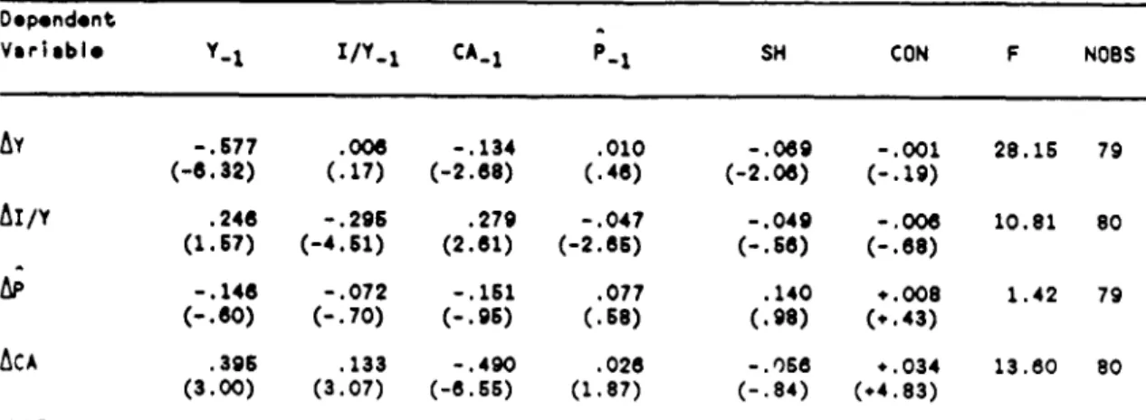
The results after one round of exclusion of influential

observations, and correcting for heteroskedacity, appear in tahle 3. 5/

The effects of participation in IMF-WB programs are measured Dy the

coefficient on the dummy CON. 7/ The first remarkable result is that

Table 3: PERFORMANCE UNDER ADJUSTMENT LENDING

Dependent

Variable Y_. I/Y_1 CA_1 P-1 SH CON F NOBS

Ay

-.677 .006 -.134 .010 -.069 -.001 28.15 79 (-6.32) (.17) (-2.68) (.46) (-2.06) (-.19) AI/Y .246 -.296 .279 -.047 -.049 -.006 10.81 80 (1.67) (-4.61) (2.61) (-2.65) (-.66) (-.68)

A;

-.146 -.072 -.161 .077 .140 +.008 1.42 79 (-.60) (-.70) (-.96) (.68) (.98) (+.43) ACA .396 .133 -.490 .026 -.068 +.034 13.60 80 (3.00) (3.07) (-6.55) (1.87) (-.84) (.4.83)

The constant term is omitted from the results, and the t-statistics are in parentheses. Definition of variables: all variables are average values over 1982-6 (e.g., y is average GDP growth during 1982-6). All lagged values are average values over 1978-81.

Y = CDP growth; I/Y = INV/GDP; CA = CA/GDP; P is the inflation rate; SH is the

external shock estimate from equation 4; CON = dummy variable with value 1 if participating in IMF and/or World Bank adjustment programs; F = statistic; NOBS = number of observations used in regression.

Results are corrected for heteroskedasticity by weighing each observation by the inverse of its estimated standard error. Extreme influential observations are excluded using Belsley, Kuh, and Welsch (1980) criteria outlined in the Appendix. The list of excluded countries are given in table A.2 of the appendix.

a significant manner, after having controlled for the negative influence of

external shocks. We also find that adjustment lending is positively

correlated with the current account performance. These results echo those

in Khan (1988) where countries that participated in Fund programs had

significantly lower output growth in the first year after the inception of

the program, but this negative effect appeared to diminish when Khan

allowed the effects of Fund programs to last two years. Khan also found

that countries participating in Fund programs had a significant improvement

in their current account. The fact that we measure performance over a

three to five year period (depending on when the country received its first

adjustment loan) may therefore account for our finding an insignificant

effect of Bank-Fund participation on growth.

The investment equation suggests that external shocks and the control group dummy are insignificant although all other variables in the equation have statistically coefficients with the expected signs. Finally, the inflation equation performed poorly. None of the explanatory variables

had a significant impact on inflation. This is probably because we have

not included credit in our instrument set. However, in that equation,

external shocks has the right sign, i.e. external shocks push up inflation. Our results also indicate that initial conditions play a crucial role in affecting the macroeconomic performance of the economy. For instance, it is found that a higher current account surplus and a lower inflation rate are associated with a better investment performance in the following period. It is, however, more difficult to understand why lagged inflation should have a positive effect on growth and on the current account.

To summarize, against the background of overall worsening

indicators for developing countries as a whole, after controlling for

external factors, IMF-WB supported adjustment programs appear not to have

significantly affected output growth, nor to have affected the level or

efficiency of investment. We conclude that the evidence on whether the

growth-oriented adjustment programs of the eighties helped recipient

countries achieve higher growth and improved efficiency is still

inconclusive. Given that the structural reforms advocated by these

programs often require a relatively long time period before their benefits

materialize, the above results are not surprising. However, a major

motivation of the adjustment programs was to mobilize resources, that is to

increase the volume of investment as well as to increase its efficiency

use. Therefore, in the next section we analyze further aggregate

investment behavior over a long time period for a group of 15 countries

which received a relatively large number of World Bank loans (usually 3 or

more). In particular, we look for instability in the investment/output

relationship after the inception of adjustment lending with a view to detect joint changes in capacity utilization due to stabilization and changes in the productivity of capital due to reforms. 8/ We also estimate output loss from investment cuts during adjustment.

5. Sustainability of Adjustment: Output Loss Estimates from Investment Cuts for a Group of Intensive Adjustment Lending Recipients

The previous results suggest that the foundations for sustained recovery were not acvieved primarily due to the fall in investment during

the adjustment lending period. We now investigate further the issue of

output during adjustment for a group of countries which were intensive

recipients of IMF-WB adjustment. 9/ We use a simple aggregate growth model

in which the only binding factor on output is capital, a simplification

which allows us to extend the analysis to a larger number of countries

because data requirements are few, and to a period of 25 years. Labor .s

assumed to be in abundant supply. Foreign exchange may be scarce, but lack

of its availability is, as in Taylor (1979), fully reflected in (lower)

investment. As derived in the appendix, the estimated equation is:

(5) Qt = (1-X) Qt-l + a It + vt

where Qt = output produced during t

X = depreciation rate

a = output capital ratio

It = investment during period t

vt = error term

This formulation eliminates the need to depend on unreliable and incomplete data on employment. It also implicitly assumes that during the estimation period, capital stock resources were fully utilized except for a stochastic term. Since this assumption is less tenable for the adjustment years, initial estimation is carried out for the pre-adjustment period. Stability testing (see table A3) is then used to assess whether the sample

period can be extended up until 1986. In addition we test whether Qt-l is

correlated with the error term and for possible endogeneity of It. Details of the estimation procedure are described in the appendix.

rta.e 4; irE fRGV'U(&J'N FUNCTION

-75 J/ IT2 Stability Period of Bi-aMi

(l-X) a D75 d/ 2 (1) c/ Estimation Year Ch;l / (2) .83 .64 .36 .94 U 82-81 81 (7.89) (2.34) (2.8) Colombia (2) .89 .53 1.0 S 8d-85 84 (8.79) (.92) Ghana (4) .82 .2S .71 S 61-86 81 (7.68) (.78) Jamaica (8) .84 .36 .94 S 61-88 SC (18.94) (3.13) C2te d'Ivoire (3) .89 .32 .98 U 88-79 79 (fixed) b/) (20.31) (2.27) Kenya (3) .96 .24 .99 S 88-88 81 (29.8) (1.88) Korea (3) .84 .60 1.0 S el-88 So (8.50) (2.48) 4aiawi (4) .94 .28 .99 U 61-80 80 (32.56) 2. 91) 4exico (2) .79 .83 1.0 U 62-81 81 (8.22) (2.93) Vorocco (3) .96 29 S9 S 81-86 82 (17.53) (1.47) Pakistan (4) .97 .84 1.0 S 81-88 79 (26.13) (2.88) Philippines (3) .90 .45 1.0 U 81-79 79 (5.90) (1.14) Thailand (2) .9e .37 1.0 S 81-86 81 (64.7) (4.85) Zambia (3) .90 0o .92 S 61-8B 83 (16.94) (1.09)

Notes: t-statistics in parenthes,s

a/ Number of SALs and SECALS n :aSertress.

b/ For all countries, gross domestic neestmert was used for It ksee eqat rn 5) except. for CSte d'Ivoire where fixed nvestment was sed.

/ S: stable equation (the break year is pr or to the first Bank adj.s "e't carn) U: unstable equation.

Estimation results and estimation periods appear in table 4.

Column (2) gives the estimate of one minus the depreciation rate, and

column (3) the inverse of the ICOR (A). With the exception of

Zambia,

the

ranZe of estimated values are in accordance with a priori expectations,

althcugh the average estimate for the depreciation rate (10?) is somewhat

on the high side. However. our interest is primarily with the estimate of

the ICOR which is around 3 (excluding outlier Zambia). For the 13 reported

countries, the values of the ICOR lend themselves to be separated into 2

groups: countries with ICORs above 3 (Kenya. Ghana, Malawi, Morocco, C5te

d'Ivoire) and countries with ICORs below 3 (Thailand, Philippines,

Colombia, Chile, Korea, Jamaica, Mexico, Pakistan). In general, the

composition of each group fits with a priori expectations.

Stability tests (reported in the appendix in table A3) indicate

that 9 out of 14 equations are stable. In interpreting this result, it

should be remembered that two factors are likely to affect the 1COR _uring

the adjustment period: ("l changes in capacity utilization due to

stabilization; _{and. .') changes in the productivity of _apita! ue tC}

reforms or to a -hange in the public and private sector shares in

investment. Because these two effects on the ICOR are indistinguishable in

cur model and because they are likely to move in opposite directions during

adlustment, it is nct surprising that stability could not be rejected in

the majority of cases. Furthermore, even when the equation was f,;end to be

unstable, the fitted value of cutput based on the pre-adjustment estimates

did not deviate much from actual output during adjustment. This suggests

that the net effect on output nf changes _n capacity utili-at:cn and

capital productivity was not significant. Therefore. instead, w4e shai'

during the adjustment period. This implies that we cannot evaluate, as

intended, whether adjustment lending raised the marginal efficiency of

investments through reforms in the system of production and investment

incentives for the private sector and, for the public sector, through

rationalization of public investments,

To estimate the output loss during adjustment. we estimated what

output would have been, had the average investment-output ratio (I7Q)

between 1970 and the initiation of Bank adjustment lending prevailed

afterwards. Formally, yearly output loss, Lt, is calculated as:

.6) Lt a(t t

*where I (I!Q) * Q., and a is the estimated value of the output/capital

tI

ratio from equation 5 Ccolu;mn 2 of table 4). Notice that if cne celieves that adjustment lending led to higher efficiency in resource use and thus to a lower incremental capital output ratio (i.e. a higher value of A),

then equation 6

will

significantly underestf.mate the output loss iue to

the

fall in investment.

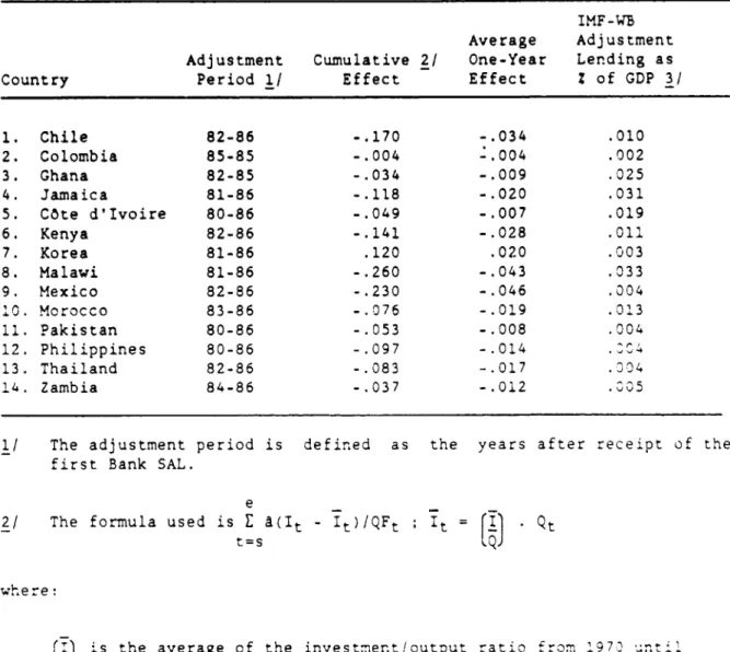
Table 5 gives the estimates of the contractionary le,ss on -,ut.ut

due to the lower investment levels during the period of adjustment :

For example, Chile lost ;7Z of output during 1982-6 tbecause of lower

investment levels. Mexico, Chile and Malawi experien?ed trhe worst losse

CDf course. one ioannct ascribe the entire Output loss -o the ajustnent

relatively -more unfavorable exterr.a envircr-ment in the early cightie.

'.hile and Mexico. for example, had tu a'so adjus: to the dlsequiL; rA

Table 5: OUTPUT LOSS DUE TO LOWER INVESTMENT

IMF-WB

Average Adjustment

Adjustment Cumulative 2/ One-Year Lending as

Country Period 1/ Effect Effect Z of GDP 3/

1. Chile 82-86 -.170 -.034 .010 2. Colombia 85-85 -.004 - .004 .002 3. Ghana 82-85 -.034 -.009 .025 4. Jamaica 81-86 -.118 -. 020 .031 5. Cote d'Ivoire 80-86 -.049 -. 007 .019 6. Kenya 82-86 -.141 -. 028 .011 7. Korea 81-86 .120 .020 .003 8. Malawi 81-86 -.260 -. 043 .033 9. Mexico 82-86 -.230 -. 046 .004 10. Morocco 83-86 -.076 -.019 .013 11. Pakistan 80-86 -.053 -. 008 .004 12. Philippines 80-86 -.097 -. 014 13. Thailand 82-86 -.083 -.017 .J04 14. Zambia 84-86 -.037 -.012 .005

1/ The adjustment period is defined as the years after receipt of the

first Bank SAL.

e

2/ The formula used is E a(It - It)/QFt ; It = [I)l

t=s tQ

where:

[i) is the average of the investment/output ratio from 197' unti!

isthe starting dates of the ad4ustment program.

. = the level of investments.

QFt = the fitted value of output (e.g. 5 where it was replaced

by It)

s = the starting date of the adjustment program.

e = the last year available during the adjustment program.

Only Korea raised her investment ratio during adjustment, thereby showing a

positive output gain.

Excluding Korea and Zambia, the countries fall into three groups:

low, medium, and high output loss as a percent of GDP. Colombia, Ghana,

Cote d'Ivoire and Pakistan lost, on average, less than one percent of GDP

per year. At the other extreme, Mexico, Malawi, Chile, and Kenya, on

average, lost close to four percent of GDP per year. In interpreting this

result, one must remember that for unstable countries (Cote d'Ivoire,

Mexico, Malawi, and Chile), the estimate of the output loss may be biased

in an unpredictable direction because of a change in the value of a during

the adjustment period.

In spite of these caveats, our results suggest a sizeable output

loss because of lower aggregate investment levels during the period of

adjusti:nt under IMF-WB lending. Since an objective of these

growth-oriented programs was to r store growth by, among others, raising invest-ment, one must ask what causes this sharp decline in investment and resulting output loss. While our analysis does not allow us to measure by how much private investment actually fell, the estimated fall in aggregate

investment output ratios was large enough in most countries t'9 leave little

doubt that private investment fell substantially during the adjustment. At least two factors must have contributed to the fall in private investment.

The first factor is that the expenditure-switching policies that accompanied the adjustment programs resulted in an increase in the relative price of imported capital goods. This cost increase was caused by the real exchange rate devaluation required to achieve a trade balance surplus to

service the external debt. Furthermore, the interpretation of the

scarce foreigrn _{exchange was probably tied up in purchasing intermediate}

goods with little left for capital goods imports.

But this interpretation does not tecognize that, given capital

investment partially _{irreversible because of sunken costs of entry and}

exit, the decision to invest in the activities supposedly made more

profitable by the ongoing reforms depends on the probability of a policy

reversal during the lifetime of the new investment. With costly resource

reallocation, uncertainty is likely to have led many private investors to

either keep their capital abroad or in existing activities until the

subjective probability that the reforms and adjustment programs will not be

reversed _{is high enough for them to commit to new investments. 10/ Thus,}

the second factor would ascribe much of the fall in private investment to

the lack of credibility in the adjustment programs, perhaps mostly because

of the size of the required adjustment, or perhaps also because of overambitious reforms in an unsettled macroeconomic environment.

6. Conclusions

This paper has provided a statistical analysis of performance under IMF-WB growth-oriented adjustment programs. The evaluation was based on a comparison of the average values of economic indicators during 1982-86

with the corresponding average values during 1978-81. The methodology

controlled for the state of the external environment during the period when growth-oriented adjustment programs were in effect as well as for the initial conditions of the loan recipient countries. Account was also taken of the policies that would have been adopted had they not participated in IMF-WB adjustment programs.

Admittedly the methodology is crude, even though it controls for

most of the pitfalls common in such comparative exercises. We found that

initial conditions played a significant role in affecting macroeconomic

performance. For example, we found that a higher current account surplus

and a lower inflation during 1978-81 were associated with a better

investment performance during 1982-86. We also found that a deterioration

in the external environment during 1982-86 was associated with lower growth

during that period.

The main result from our comparisons between IMF-WB recipients and

countries that did not receive adjustment loans (or received them towards

the end of the period so that not enough time had elapsed to include them

among loan recipients) relate to growth and investment. After controlling

for initial conditions and external factors, we found no evidence of a

statistically better (or worse) performance for loan recipient countries.

These results suggest that the expected positive effects on growth and

resource mobilization expected from adjustment with growth packages and not

yet occurred. Given that the structural reforms advocated by these

programs often require a relatively long time period before their benefits

materialize, these results may not be surprising.

In the last section of the paper we analyzed in greater detail the

investment output relationship for a group of 14 countries that received a

large amount of growth-oriented adjustment lending. For each country, we

fit a simple production function (in which capital is the only constraint

on growth) over a 25 year period. We then provided an estimate of the

output loss from the shortfall in investment during the period when each

country was receiving adjustment lending. The results show much foregone

during the period of adjustment. Thus, the desired signs of a sustainable

recovery through _{higher investment, evaluated here through 1986, were not}

Footnotes

1/ In previous work (Faini et. al. 1989), we evaluated performance undet

adjustment lending for a group of nine indicators using a

before-and-After approach so that we did not control for initial conditions nor

for the size of external shocks.

2/ The World Bank initi-ated SALS (structural adjustment loans) and SECALs

(sectoral adjustment loans) in 1979 and 1981 respectively. Like the

EFF (Extended Fund Facility) and stand-by arrargements, World Bank

adjustment loans are quick disbursing loans. For a description of

adjustment lending investments by the IMF (World Bank) see IMF (1987),

World Bank (1989). All IMF upper credit tranche programs are of short

duration and some Funid-supported adjustment programs were initiated

before 1979. However, of 288 programs during 1973-86, only 44 took

place during 1973-78.

3/ The following model draws on Goldstein and Montiel (1986).

4/ Because the choice of cut-off is arbitrary, we also carried out our

estimation using 1981 as an alte:native cut-off point. The results were s.milar to those reported in table 3.

5/ The formula derives from a two-period maximization by firms and

households under assumptions of perfect competition and wage-price flexibility. See Dornbusch (1985, pp. 354-6).

6/ One round of exclusion tests results in about 5 percent loss of

observations. Excluded countries are reported in the appendix in Table A.2. The exclusion criteria were determined by the value of Cook's D-statistic. See Belsley, Kuh and Welsch (1980), and section A.3.

7/ Similar results, not reported here, were obtained in an alternative

estimation based on a model in which CON is replaced by the intensity of IMF-WB adjustment lending.

8/ Because we fit the growth model to a relatively large number of

countries, we kept it as simple as possible so that we were not able to distingu_sh between capacity and productivity effects nor between private and public investment.

9/ The 14 countries (see Table 4) were selected on the basis of the

number of SALs. Turkey, included in that sample, had to be dropped from our analysis because regime changes did not allow us to get stable estimates.

10/ This interpretation is emphasized in a broader context in the

References

Balassa, B. 1988. "Quantitative Appraisal of Adjustment Lending," PPR

Working Paper Series No. 79.

Belsley, D. Kuh and Welsch. 1980. Diagnostic Tests in Regression

Analysis.

Blejer, D. and M. Ki.an. 1984. "Government Policy and Private Investment

in Developing Countries," IMF Staff Papers, 31, 2, 379-403.

Buffie, E. 1984. 'The Macroeconomics of Trade Liberalization," Journal oi International Economics, Vol. 17, pp. 121-S7.

Buffie, E. 1986. "Devaluation, Investment and Growth in LDCs," Journal of Development Economics, Vol. 20, pp. 361-79.

Calvo, G. 1986. "Incredible Reforms," mimeo, University of Pennsylvania.

Cline, W.R. 1985. "International Debt: Fror. Crisis to Recovery,'

American Economic Review, pp. 185-90.

Corbo, V., M. Goldstein, and M. Khan, eds. 1988. Adjustment with Growth, IMF, Washington, D.C.

Corden, M. 1988. "Macroeconomic Adjustment in Developing Countries, IMF

(mimeo).

Cornia, G., R. Jolly, and F. Stewart. 1987. Adjustment with a Human Face, Vol. 1. Oxford University Press.

Dadkhah, K.M. and F. Zahedi. 1986. 'Simultaneous Estimation of Production Functions and Capital Stocks for Developing Countries,' The Review of Economics and Statistics, Vol. LXVIII, No. 3, pp. 443-51.

Dell, S. 1983. "Stabilization: The Political Economy of Overkill,' in J.

Williamson, ed., IMF Conditionality, pp. 7-46. Institute for

International Economics, Washington, D.C.

Diaz-Alejandro, C. 1979. "Southern Cone Stabilization Problems, in W.

Cline and S. Weintraub, eds., Economic Stabilization in Developing Countries, Washington, D.C.

Donovan, D.J. 1981. 'Real Responses Associated with Exchange Rate Action in Selected Upper Credit Tranche Stabilization Programs," Staff Papers, pp. 698-727.

Dornbusch, R. 1985. "Policy and Performance Links Between LDC Debtors and Industrial Nations," Brookings Papers on Economic Activily, No. 2, pp. 303-68.

Dornbusch, R. 1986. "The Effects of OECD Macroeconomic Policies on Non-Oil Developing Countries," World Bank Staff Working Papers, No. 793, World Bank.

Dornbusch, R. 1988. "Notes on Credibility and Stabilization," mimeo, MIT.

Faini, R., J. de Melo, A. Senhadji-Semlali, J. Stanton. 1988.

'Performance Under Adjustment Lending,' forthcoming in V. Thomas, A. Chhibber, M. Dailami, and J. de Melo, eds., Structural Adjustment and the World Bank, Oxford University Press.

Genberg, A. and A.K. Swoboda. 1987. 'The Medium-Term Relationship Between

Performance Indicators and Policy: A Cross Section Approach," EPD

Discussion Paper No. EPD-01, The World Bank.

Goldstein, M. and P. Montiel. 1986. "Evaluating Fund Stabilization

Programs with Multicountry Data: Some Methodological Pitfalls," IMF

Staff Papers, Vol. 33, No. 2, pp. 314-44.

Hausman, J.A. 1978. 'Specification Tests in Econometrics,' Econometrica,

Vol. 46, pp. 1257-70.

Khan, M. 1988. "The Macroeconomic Effects of Fund-Supported Adjustment

Programs: An Empirical Assessment," (mimeo), IMF.

Khan, M. and M. Knight. 1981. "Stabilization Programs in Developing

Countries: A Formal Framework," Staff Papers, Vol. 28, No. 1, .p. 1-53.

Kiviet, J.F. 1985. "Model Selection Test Procedures in a Single Linear

Equation of a Dynamic Simultaneous System and Their Effects in Smal' Samples," Journal of Econometrics, Vol. 28, 327-62.

Kiviet, J.F. 1986. "On the Rigour of Some Mispecification Tests for

Modelling Dynamnic Relationships," Review of Economic Studies,

pp. 241-61.

Mitra, P.K. 1984. "Adjustment to External Shocks in Selected

Semi-Industrial Countries, 1974-1981," mimeo, Public Economics Division, The World Bank.

Rodrik, D. 1988. 'Liberalization, Sustainability, and the Design of

Structural Adjustment Programs," mimeo, The World Bank.

Sachs, J. and H. Huizinga. 1987. "U.S. Commercial Banks and the

Developing Country Debt Crisis," Brookings Papers on Economic

Activity.

Sargan, J.D. 1958. "The Estimation of Economic Relationships Using

Instrumental Variables," Econometrica, Vol. 26, pp. 393-415.

van Wijnbergen, S. 1982. "Stagflation Effects of Monetary Stabilization

Policies: A Quantitative Analysis of South Korea," Journal of

van Wijnbergen, S. 1986. wExchange Rate Management and Stabilization

Policies _{in Developing Countries," Journal of Development Economics,}

Appendix

1. Data Sources

All data were extracted from the World Bank's BESD and ANDREX data bases except the SAL and SECAL flows which were extracted from World Bank publications. Data in constant dollars were obtained by using the World

Bank's atlas exchange rate conversion factor. In the calculation of

external shocks (equation 4), terms of trade indices were obtained by dividing current exports and imports (expressed in dollars) by the constant values. Similar results were obtained when the terms-of-trade indices were calculated from current an,i constant local currency values from National Accounts data.

To calculate th.e effective interest rate on external debt, we

applied LIBOR + 1 to the share of total non-concessional debt and the

implicit interest rate from interest payments on concessional debt. For Bank-Funding (BF) we constructed two variables; one based on gross IMF credit (results in table 1); another in the net IMF credit where IMF credit was calculated as IMF purchases less IMF repurchases. In both cases, Bank

SAL credits are the sum of SAL + SECAL commitments. We did not report the

results based on the net TMF credit definition because they are extremely

close to those obtained with gross credit.

As mentioned in the text, we also experimented with a formulation in which we replaced the dummy control group variable CON in equation (3) with a measure of the intensity of IMF-WB credit. In those regressions (not reported in the text because they were similar with those discussed in

credit (SAL + SECAL) during 1982-86, expressed as a percentage of average GDP during 1982-86.

2. Sample

Table A.1 lists the 93 countries in the sample along with their classification. The control group, denoted by C, includes 41 countries of which 6 countries received adjustment lending in 1986, the last year of available data and 3 which received their first adjustment credit in 1984.

A'll other countries received IMF and/or World Bank adjustment credits

between 1982 and 1984. Of the 50 countries which received adjustment

credits during this period, 2v. countries initiated their first adjustment

credit in 1982 and 24 irn 1983.

3. Excluded Countries Trc. 7atle A.:

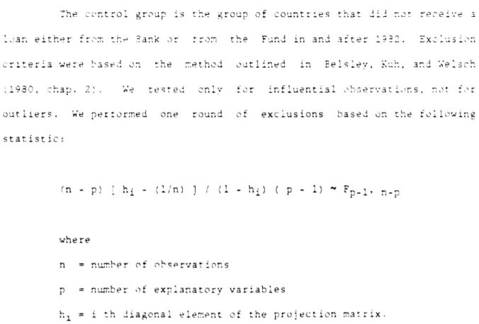
"he -ntro. grou is tI e group of cou.ntr es tha JA _,o r e_

:.ar. eitr.er ear.k :r;. r;r ar rrc the Fun<;d in an art er 1 2. EX_' s

criterla we-e onased o. the -.ethod octl ned in Eelslee, :K, and n iel a.h

;1433, hap. 2' tested only e r irnfluernt al ? rvat c r,s, .

outliers. We 7ert rored one round of excLusions based orn roe fol Lowiniz

statistic:

(n - p) hi - (ln) ] / (1 - hi) ( p - ) Fp , - p

whe re

n = number of observations

p = rnm.ber of exp.anatory variables

Table A.1: 93 COUNTRIES IN SAMPLE Nation 'lation (F,B) ArgentinA (F,B) Morocco C Burundi (F,B) Madagascar C Benin (F,B) Mexico F Bangladesh F Mali C Bolivia C Malta (F,B) Brazil C Mauritania F Barbados (F,B) Mauritius C Burma (F,B) Malawi C Botswana C Malaysia

(F,B) Central African Republic (F,B) Niger

(F,B) Chile B Nigeria

C China C Nicaragua

(F,B) C6te d'Ivoire C Nepal

C Cameroon (F,B) Pakistan

C Congo (F,B) Panama

B Colombia F Peru

(F,B) Costa Rica (F,B) Philippines

C Cyprus C Papua New Guirea

F Dominican Republic F Portugal

C Algeria C Raraguay (F,B) Ecuador _ a C Egypt -C Ethiopia J',B Se &gat C Fiji _ n a e Gabon '-a (F,B) Ghana C Guinea 'S -m Gambia B Guinea-Bissau S , C Greece F Guatemala C Guyana -C Hong Kong F Honduraas F Haiti (F,B) Hungary C Burkina Paso r C I donesia F India C Z- C Israel (F,B) Jamaica C Jordan (F,B" 's V i (F,B) Kenya (F,B) Korea (F,B e F Liberia $F,Ba

F Sri Lanka (F.B)

BI-C Lesotho

N4otes- F,B denote IMF an' 'WB loan, rec±pients respe:;.-el; d.r -. *.e

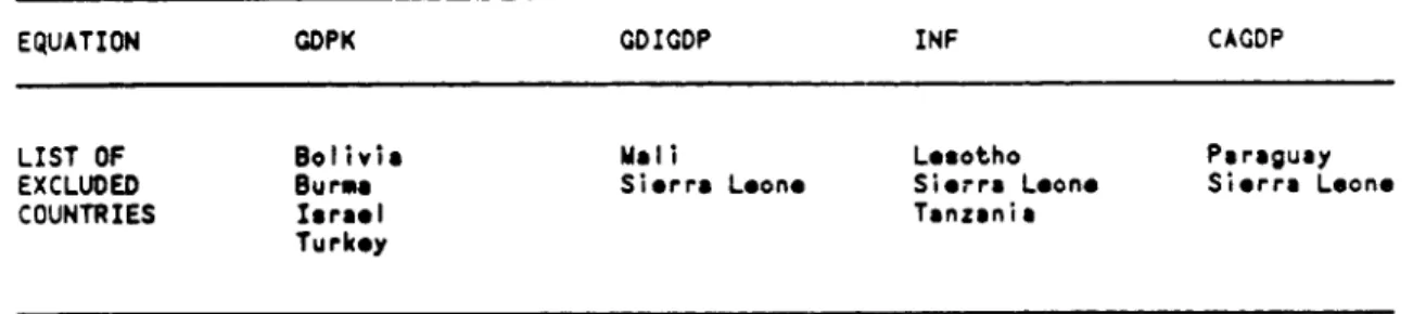
Table A.2: COUNTRIES EXCLUOED FROM PERFORMANCE REGRESSIONS

EQUATION GDPK GDIGDP INF CAGDP

LIST OF Bolivia Mali Lesotho Paraguay

EXCLUDED Burea Sierra Leone Sierra Leone Sierra Leone

COUNTRIES Israel Tanzania

For p > 10 and n - p > 50, the value of the F at 95Z confidence level is

less than 2 and hence 2 p/n is a good rough cut-off. We took into account

two criteria: (a) no more than 5Z of the observations should be excluded:

and (b) exclude observations for which hi > 2 p/n.

Table Al lists the 93 countries in the sample. Table A2 gives the

list of influential observations excluded from each equation.

4. Production Function Estimation

Estimation of the production function relied on a strategy to

detect the presence of correlation of Qt-l with the error term and to check

for endogeneity of It. An instrumental variable (IV) method, described

below, was used if either Qt-l or It were found to be endogenous.

Under the assumption that capital (Kt) is the only binding factor,

output (Qt) can be written as Qt = aKt + Ut where ut is a stochastic term.

Lag the expression for Qt by one period, multiply the resulting expression for Qt-l by one minus the depreciation rate X, then subtract (l-X)Qt.l from Qt. Using the capital stock identity yields equation 5 in the text. The model draws on Dadkhah and Zahedi (1986).

The error term in eq. 5 vt is equal to ut-(l-X)vtil. Therefore, unless the error term ut follows a first-order autoregressive process with parameter p=l-X. OLS estimation will yield inconsistent estimates because of correlation of Qt-l with the error term. The possible endogeneity of It in (5) may also result in inconsistent estimates. This led us to adopt the following estimation strategy.

First, we estimated (5) by OLS for the fourteen countries

performing the Lagrange multiplier (LM) test for autocorrelation to check

the LM test, an instrumental variable (IV) procedure was used with It-1 and

domestic credit as instruments _{for Qt-l. In the case where endogeneity of}

It-, was detected alone with autocorrelation, we used It-2 and domestic

credit as instruments for Qt-l Table A.3 gives the precise set of

instruments _{used in each equation estimated by IV. Finally, in checking}

for endogeneity of It. we used the Hausman (1978) test on OLS equations and

the Sargan (1958) test on the instrumental variable equations.

To sum up, we used OLS if neither Qt-l nor It were shown to be

endogenous. An instrumental variables technique was used otherwise, with

the set of instruments depending on which variable was detected endogenously, (Qt-l and/or It), and on the eventual presence of autocorrelation.

To test for stability we used both the Chow and the Hendry

procedures for OLS estimates, and we relied on the modified Chow test

(Kiviet, 1985) in the context of IV estimation. In deciding whether an

equation was stable or not, we allowed for the fact that the power of the

Chow test may be fairly low, while the actual size of the Hendry test may

Tablo A.3

Estimation LU2 Chow Hendry Sargan Godfrey Set of

Technique (X 1) instruments IV Chile 13.6 .28(XI) 008 B (.02) (.9(X) IV Colombia 1.31 1109(X.) .09 A (.26) (.30) OLS Ghana .08 .08 1.33 1.35 (.78) (.30) (.8S) OLS Jamaica .02 .02 .74 .94 (.89) (.54) (.82)

OLS Cote d'Ivolre 2.06 2.06 4.48 5.67

(fixed) (.15) (.01) (.68) OLS Kenya .18 .18 .49 3.36 (.67) (.78) (.64) OLS Korea (1) 9.51 9.61 1.98 4.80 (.002) (.13) (.67) OLS Malawi .48 .48 2.69 3.08 (.49) (.05) (.80) IV Mexico 17.18 22.4(XI1) 2.24 D (.004) (.13) IV Morocco 7.3 4.03(Xi) 4.03 C (12.2) (.04) OLS Pakistan 1.89 1.69 1.61 2.90 (.19) (.23) (.89) IV Philippinos 19.2 O(Xf) 0 A (.01) (.99) OLS Thailand 1.39 1.39 .84 1.42 (.24) (.64) (.92) OLS Zambia 2.24 2.24 .11 .11 (.09) (.99) (1.0) A: I, I(-1), DC C: I(-1), DC, Q(-2)

8: I, I(-I), Q(-2) D: I(-I), DC, DC(-I), Q(-2) For tho definition of the variabloe see section A.4.

(1) Tho LV is quite high for Koroa which indicatos tho presence of autocorrelation. Normally, the IV tochnique would havo boon employod but did not give reasonable estimate. Hence, OLS estimat.. are reported.

Significance level for chi-squared statistic:

2 2 X2 = 3.84 X 2=6.63 1,a = o0 1,a = .01 2 2 X2 = 6.99 X = 9.21 2 = a.o5 2,a = .01

itle Date fLo paper

WPS402 The GATT as International Discipline J. Michael Finger March 1990 N. Artis

Over Trade Restrictions: A Public 38010

Choice Approach

WPS403 Innovatlle Agricultural Extensicn S Tj p Walker June 1990 M. Villar

for Women: A Case Study of 33752

Cameroon

WPS404 Chile's Labor Markets in an Era of Luis A. Riveros April 1990 R. Luz

Adjustment 34303

WPS405 Investments in Solid Waste Carl Bartone Apri! 1990 S. Cumine

Management: Opportunities for Janis Bernstein 33735

Environmental Improvement Frederick Wright

WPS406 Township, Village, and Private William Byrd April 1990 K. Chen

Industry in China's Economic Alan Gelb 38966

Reform

WPS407 Public Enterprise Reform: Ahmed Galal April 1990 G. Orraca-Tetteh

A Challenge for the World Bank 37646

WPS408 Methodological Issues in Evaluating Stijn Claessens May 1990 S. King-VVatson

Debt-Reducing Deals Ishac Diwan 33730

WPS409 Financial Policy and Corporate Mansoor Dailami April 1990 M. Raggambi

Investment in Imperlect Capital 37657

Markets The Case of Korea

WPS410 The Cost of Capital and Investment Alan Auerbach April 1990 A Bhalla

n Developing Countries 37699

WPS411 Institutional Dimensions of Poverty Lawrence F Salmen May 1990 E Madrona

Reduct:on 37496

WPS412 Exchange Rate Policy in Developing W Max Corden May 1990 M. Corden

Countries 39175

WPS413 Supporting Safe Motherhood L M. Howard May 1990 S. Ainsworth

A Review of Financial Trends 31091

Full Report

WPS414 Supporting Safe Motherhood: L M. Howard May 1990 S Ainsworth

A Review of Financial Trends 31091

Summary

WPS415 How Good (or Bad) are Country Norman Hicks AorIl 1990 M. Berg

Title

~~~~~~~Author

DAIR for papa,

WPS416 Improving Data on Poverty in the Paul Glewwe May 1990 A. Murphy

Third World: The World Bank's 33750

Living Standards Measurement Study

WPS417 Modeling the Macroeconomic William Easterly May 1990 R. Luz

Requirements of Policy Reform E. C. Hwa 34303

Piyabha Kongsamut Jan Zizek

WPS418 Does Devaluation Hurt Private Ajay Chhibber May 1990 M. Colinet

Investment? The Indonesian Case Nemat Shafik 33490

WPS419 The Design and Sequencing of Brian Levy May 1990 B. Levy

Trade and Investment Policy Reform: 37488

An Institutional Analysis

WPS420 Making Bank Irrigation Investments Gerald T. OMara May 1990 C. Spooner

More Sustainable 30464

WPS421 Taxation of Financial Intermediation: Christophe Chamley May 1990 W.

Pitayato-Measurement Principles and Patrick Honohan nakarn

Application to Five African Countries 37666

WPS422 Civil Service Reform and the World Barbara Nunberg May 1990 R. Malcolm

Bank John Nellis 47495

WPS423 Relative Price Changes and the M. Shahbaz Khan May 1990 WDR Office

Growth of the Public Sector 31393

WPS424 Mexico's External Debt Sweder van Wijnbergen June 1990 M. Stroude

Restructuring in 1989-90 38831

WPS425 The Earmarking of Government Wiliam A McCleary

Revenues in Colombia Evamaria Uribe Tobon

WPS426 Growth-Oriented Adjustment Riccardo Faini June 1990 M. Ameal

Programs: A Statistical Analysis Jaime de Malo 37947

Abdel Senhadji-Semlali Julie Stanton

WPS427 Exchange Reform, Parallel Markets Ajay Chhibber May 1990 M. Colinet

and Inflation in Africa: The Case Nemat Shafik 33490

of Ghana

WPS428 Perestroyka and Its Implications Bela Balassa May 1990 N. Campbell