Inference for high-dimensional sparse econometric models

Inference for high-dimensional

sparse econometric models

A. Belloni

V. Chernozhukov

C. Hansen

The Institute for Fiscal Studies

Department of Economics, UCL

MODELS

A. BELLONI, V. CHERNOZHUKOV, AND C. HANSEN

Abstract. This article is about estimation and inference methods for high dimensional sparse (HDS) regression models in econometrics. High dimensional sparse models arise in situations where many regressors (or series terms) are available and the regression function is well-approximated by a parsimonious, yet unknown set of regressors. The latter condition makes it possible to estimate the entire regression function effectively by searching for approximately the right set of regressors. We discuss methods for identifying this set of regressors and esti-mating their coefficients based onℓ1-penalization and describe key theoretical results. In order

to capture realistic practical situations, we expressly allow for imperfect selection of regressors and study the impact of this imperfect selection on estimation and inference results. We focus the main part of the article on the use of HDS models and methods in the instrumental vari-ables model and the partially linear model. We present a set of novel inference results for these models and illustrate their use with applications to returns to schooling and growth regression. Key Words: inference under imperfect model selection, structural effects, high-dimensional econometrics, instrumental regression, partially linear regression, returns-to-schooling, growth regression

1. Introduction

We consider linear, high dimensional sparse (HDS) regression models in econometrics. The HDS regression model allows for a large number of regressors,p, which is possibly much larger than the sample size, n, but imposes that the model is sparse. That is, we assume only s ≪ n of these regressors are important for capturing the main features of the regression function. This assumption makes it possible to estimate HDS models effectively by searching for approximately the right set of regressors. In this article, we review estimation methods for HDS models that make use of ℓ1-penalization and then provide a set of novel inference results. We also provide empirical examples that illustrate the potential wide applicability of HDS models and methods in econometrics.

Date: First version: June 2010, This version is of December 30, 2011.

The preliminary results of this paper were presented at V. Chernozhukov’s invited lecture at 2010 Econometric Society World Congress in Shanghai. Financial support from the National Science Foundation is gratefully acknowledged. Computer programs to replicate the empirical analysis are available from the authors. We thank Josh Angrist, the editor Manuel Arellano, the discussant Stephane Bonhomme, and Denis Chetverikov for excellent constructive comments that helped us improve the article.

The motivation for considering HDS models comes in part from the wide availability of data sets with many regressors. For example, the American Housing Survey records prices as well as a multitude of features of houses sold; and scanner data-sets record prices and numerous characteristics of products sold at a store or on the internet. HDS models are also partly motivated by the use of series methods in econometrics. Series methods use many constructed or series regressors – regressors formed as transformation of elementary regressors – to approximate regression functions. In these applications, it is important to have parsimonious yet accurate approximation of the regression function. One way to achieve this is to use the data to select a small of number of informative terms from among a very large set of control variables or approximating functions. In this article, we formally discuss doing this selection and estimating the regression function.

We organize the article as follows. In the next section, we introduce the concepts of sparse and approximately sparse regression models in the canonical context of modeling a conditional mean function and motivate the use of HDS models via an empirical and analytical examples. In Section 3, we discuss some principal estimation methods and mention extensions of these methods to applications beyond conditional mean models. We discuss some key estimation results for HDS methods and mention various extensions of these results in Section 4. We then develop HDS models and methods in instrumental variables models with many instruments in Section 5 and a partially linear model with many series terms in Section 6, with the main emphasis given to inference. Finally, we present two empirical examples which motivate the use of these methods in Section 7.

Notation. We allow for the models to change with the sample size, i.e. we allow for array asymptotics. In particular we assume that p = pn grows to infinity as n grows, and s=sncan also grow withn, although we require thatslogp=o(n). Thus, all parameters are implicitly indexed by the sample size n, but we omit the index to simplify notation. We also use the following empirical process notation,En[f] =En[f(zi)] =Pni=1f(zi)/n.Thel2-norm is denoted by_k·k, and thel0-norm,k·k0, denotes the number of non-zero components of a vector. We usek · k∞ to denote the maximal element of a vector. Given a vectorδ ∈Rp, and a set of indicesT _{⊂ {}1, . . . , p_}, we denote by δT ∈Rp the vector in which δT j =δj ifj∈T,δT j = 0 if j /_∈T. We use the notation (a)+ = max{a,0}, a∨b = max{a, b} and a∧b = min{a, b}. We also use the notationa.bto denote a6cbfor some constant c >0 that does not depend on n; and a.P b to denote a=OP(b). For an event E, we say that E wp→ 1 whenE occurs with probability approaching one asngrows.

2. Sparse and Approximately Sparse Regression Models

In this section we review the modeling foundations for HDS methods and provide motivating examples with emphasis on applications in econometrics. First, let us consider the following

parametric linear regression model:

yi =x′iβ0+ǫi, ǫi ∼N(0, σ2), β0∈Rp, i= 1, . . . , n T = support(β0) hasselements wheres < n,

wherep > n is allowed, T is unknown, and regressors X = [x1, . . . , xn]′ are fixed. We assume Gaussian errors to simplify the presentation of the main ideas throughout the article, but note that this assumption can be eliminated without substantially altering the results. It is clear that simply regressingy on allp availablex variables is problematic whenp is large relative to nwhich motivates consideration of models that impose some regularization on the estimation problem.

The key assumption that allows effective use of this large set of covariates is sparsity of the model of interest. Sparsity refers to the condition that only s ≪ n elements of β0 are non-zero but allows the identities of these elements to be unknown. Sparsity can be motivated on economic grounds in situations where a researcher believes that the economic outcome could be well-predicted by a small (relative to the sample size) number of factors but is unsure about the identity of the relevant factors. Note that we allows=snto grow withn, as mentioned in the notation section, although slogp =o(n) will be required for consistency. This simple sparse model substantially generalizes the classical parametric linear model by letting the identities, T,of the relevant regressors be unknown. This generalization is useful in practice since it is problematic to assume that we know the identities of the relevant regressors in many examples. The previous model is simple and allows us to convey the essential ideas of the sparsity-based approach. However, it is unrealistic in that it presumes exact sparsity or that, after accounting for s main regressors, the error in approximating the regression function is zero. We shall make no formal use of the previous model, but instead use a much more general,

approximately sparse or nonparametric model. In this model,all of the regressors potentially have anon-zerocontribution to the regression function, but no more thansunknown regressors are needed for approximating the regression function with a sufficient degree of accuracy.

We formally define the approximately sparse model as follows.

Condition ASM. We have data _{(yi, zi), i = 1, . . . , n} that for each n obey the regression

model:

yi=f(zi) +ǫi, ǫi ∼N(0, σ2), i= 1, . . . , n, (2.1)

where yi is the outcome variable, zi is a kz-vector of elementary regressors, f(zi) is the re-gression function, and ǫi are i.i.d. disturbances. Let xi = P(zi), where P(zi) is a vector of

dimension p = pn, that contains a dictionary of possibly technical transformations of zi,

in-cluding a constant. The values x1, . . . , xn are treated fixed, and normalized so that En[x2_ij] = 1

for j = 1, . . . , p. The regression function f(zi) admits the approximately sparse form, namely

there existsβ0 such that

f(zi) =x′iβ0+ri, kβ0k0 6s, cs:={En[ri2]}1/2 6Kσ p

where s=sn=o(n/logp) andK is a constant independent of n.

In the set-up we consider the fixed design case, which covers random sampling as a special case where x1, . . . , xn represent a realization of this sample on which we condition through-out. The vector xi = P(zi) can include polynomial or spline transformations of the original regressorszi see, e.g., Newey (1997) and Chen (2007) for various examples of series terms. The approximate sparsity can be motivated similarly to Newey (1997), who assumes that the first s = sn series terms can approximate the nonparametric regression function well. Condition ASM is more general in that it does not impose that the most important s = sn terms in the approximating dictionary are the firststerms; in fact, the identity of the most important terms is treated as unknown. We note that in the parametric case, we may naturally choose x′_iβ0 =f(zi) so that ri = 0 for all i= 1, . . . , n. In the nonparametric case, we may think of x′_iβ0 as any sparse parametric model that yields a good approximation to the true regression function f(zi) in equation (2.1) so that ri is “small” relative to the conjectured size of the estimation error. Given (2.2), our target in estimation is the parametric functionx′_iβ0, where we can call

T := support(β0)

the “true” model. Here we emphasize that the ultimate target in estimation is, of course, f(zi). The function x′_iβ0 is simply a convenient intermediate target introduced so that we can approach the estimation problem as if it were parametric. Indeed, the two targets, f(zi) and x′

iβ0, are equal up to the approximation error ri. Thus, the problem of estimating the parametric target x′

iβ0 is equivalent to the problem of estimating the nonparametric target f(zi) modulo approximation errors.

One way to explicitly construct a good approximating modelβ0 for (2.2) is by takingβ0 as the solution to min β∈RpEn[(f(zi)−x ′ iβ)2] +σ2k βk0 n . (2.3)

We can call (2.3) the oracle problem,1 and so we can call T = support(β0) the oracle model. Note that we necessarily have that s = _kβ0k 6 n. The oracle problem (2.3) balances the approximation errorEn[(f(zi)−xi′β)2] over the design points with the variance termσ2kβk0/n, where the latter is determined by the number of non-zero coefficients in β. Letting c2

s :=

En[r2i] =En[(f(zi)−xi′β0)2] denote the squared error from approximating valuesf(zi) byx′iβ0, the quantity c2_s+σ2s/n is the optimal value of (2.3). In common nonparametric problems, such as the one described below, the optimal solution in (2.3) would balance the approximation error with the variance term giving thatcs 6Kσ

p

s/n. Thus, we would have pc2

s+σ2s/n. σps/n,implying that the quantity σps/nis the ideal goal for the rate of convergence. If we knew the oracle model T, we would achieve this rate by using the oracle estimator, the least squares estimator based on this model. Of course, we do not generally know T since we do 1_{By definition the oracle knows the risk function of any estimator, so it can compute the best sparse least} square estimator. Under some mild condition the problem of minimizing prediction risk amongst all sparse least square estimators is equivalent to the problem written here; see, e.g., Belloni and Chernozhukov (2011b).

not observe the f(zi)’s and thus cannot attempt to solve the oracle problem (2.3). Since T is unknown, we will not generally be able to achieve the exact oracle rates of convergence, but we can hope to come close to this rate.

Before considering estimation methods, a natural question is whether exact or approximate HDS models make sense in econometric applications. In order to answer this question, it is helpful to consider the following two examples in which we abstract from estimation completely and only ask whether it is possible to accurately describe some structural econometric function f(z) using a low-dimensional approximation of the form P(z)′β0.

Example 1: Sparse Models for Earning Regressions. In this example we consider a model for the conditional expectation of log-wage yi given education zi, measured in years of schooling. We can expand the conditional expectation of wageyi given education zi:

E[yi|zi] = p X j=1

β0jPj(zi), (2.4) using some dictionary of approximating functions P(zi) = (P1(zi), . . . , Pp(zi))′, such as poly-nomial or spline transformations in zi and/or indicator variables for levels of zi. In fact, since we can consider an overcomplete dictionary, the representation of the function using P1(zi), . . . , Pp(zi) may not be unique, but this is not important for our purposes.

A conventional sparse approximation employed in econometrics is, for example,

f(zi) :=E[yi|zi] = ˜β1P1(zi) +· · ·+ ˜βsPs(zi) + ˜ri, (2.5) where thePj’s are low-order polynomials or splines, with typically one or two (linear or linear and quadratic) terms. Of course, there is no guarantee that the approximation error ˜ri in this case is small or that these particular polynomials form the best possibles-dimensional approx-imation. Indeed, we might expect the function E[yi|zi] to change rapidly near the schooling levels associated with advanced degrees, such as MBAs or MDs. Low-degree polynomials may not be able to capture this behavior very well, resulting in large approximation errors ˜ri.

A sensible question is then, “Can we find a better approximation that uses the same number of parameters?” More formally, can we construct a much better approximation of the sparse form

f(zi) :=E[yi|zi] =βk1Pk1(zi) +· · ·+βksPks(zi) +ri, (2.6)

for some regressor indicesk1, . . . , ksselected from{1, . . . , p}? Since we can always include (2.5) as a special case, we can in principle do no worse than the conventional approximation; and, in fact, we can construct (2.6) that is much better, if there are some important higher-order terms in (2.4) that are completely missed by the conventional approximation. Thus, the answer to the question depends strongly on the empirical context.

Consider for example the earnings of prime age white males in the 2000 U.S. Census see, e.g., Angrist, Chernozhukov, and Fernandez-Val (2006). Treating this data as the population data,

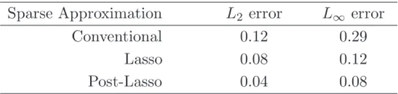
Sparse Approximation L2 error L∞ error Conventional 0.12 0.29

Lasso 0.08 0.12

Post-Lasso 0.04 0.08

Table 1. Errors of Conventional and the Lasso-based Sparse Approximations of the Earning Function. The Lasso method minimizes the least squares criterion plus the ℓ1-norm of the

coefficients scaled by a penalty parameterλ. The nature of the penalty forces many coefficients to zero, producing a sparse fit. The Post-Lasso minimizes the least squares criterion over the non-zero components selected by the Lasso estimator. This example deals with a pure approximation problem, in which there is no noise.

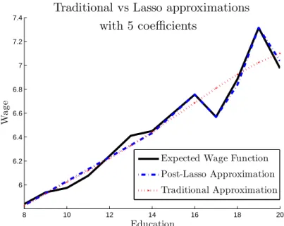
we can computef(zi) =E[yi|zi] without error. Figure 1 plots this function. We then construct two sparse approximations and also plot them in Figure 1. The first is the conventional approximation of the form (2.5) with P1, . . . , Ps representing polynomials of degree zero to s₋1 (s= 5 in this example). The second is an approximation of the form (2.6), withPk1, . . . ,

Pks consisting of a constant, a linear term, and three linear splines terms with knots located

at 16, 17, and 19 years of schooling. We find the latter approximation automatically using theℓ1-penalization or Lasso methods discussed below,2 although in this special case we could construct such an approximation just by eye-balling Figure 1 and noting that most of the function is described by a linear function with a few abrupt changes that can be captured by linear spline terms that induce large changes in slope near 17 and 19 years of schooling. Note that an exhaustive search for a low-dimensional approximation in principle requires looking at a very large set of models. Methods for HDS models, such as ℓ1-penalized least squares (Lasso), which we employed in this example, are designed to avoid this search. Example 2: Series approximations and Condition ASM. It is clear from the state-ment of Condition ASM that this expansion incorporates both substantial generalizations and improvements over the conventional series approximation of regression functions in Newey (1997). In order to explain this consider the set_{Pj(z), j>1} of orthonormal basis functions on [0,1]d, e.g. orthopolynomials, with respect to the Lebesgue measure. Suppose zi have a uniform distribution on [0,1]d for simplicity.3 _{Assuming E[f}2_(z

i)] < ∞, we can represent f via a Fourier expansion, f(z) =P∞_j=1δjPj(z), where{δj, j >1} are Fourier coefficients that satisfyP∞_j=1δ2j <∞.

Let us consider the case that f is a smooth function so that Fourier coefficients fea-ture a polynomial decay δj ∝ j−ν, where ν is a measure of smoothness of f. Consider 2_{The set of functions considered consisted of 12 linear splines with various knots and monomials of degree} zero to four. Note that there were only 12 different levels of schooling.

3_{The discussion in this example continues to apply whenz}

i has a density that is bounded from above and

8 10 12 14 16 18 20 6 6.2 6.4 6.6 6.8 7 7.2 7.4

Traditional vs Lasso approximations

W

a

g

e

Education

Expected Wage Function Post-Lasso Approximation Traditional Approximation

with 5 coefficients

Figure 1. The figures illustrates the Post-Lasso sparse approximation and the fourth order polynomial approximation of the wage function.

the conventional series expansion that uses the first K terms for approximation, f(z) = PK

j=1β0jPj(z) +ac(z), with β0j = δj. Here ac(zi) is the approximation error which obeys p En[a2c(zi)] .P p E[a2 c(zi)] . K −2ν+1

2 . Balancing the order K− 2ν+1

2 of approximation error

with the order pK/n of the estimation error gives the oracle-rate-optimal number of series termss=K ∝n1/2ν, and the resulting oracle series estimator, which knowss, will estimatef at the oracle rate ofn1−4ν2ν. This also gives us the identity of the most important series terms

T=_{1, ..., s_}, which are simply the first sterms. We conclude that Condition ASM holds for the sparse approximationf(z) =Pp_j=1β0jPj(z) +a(z), withβ0j =δj forj6sandβ0j = 0 for s+ 16j6p, and a(zi) =ac(zi), which coincides with the conventional series approximation above, so thatpEn[a2(zi)].P

p

s/nand _kβ0k0 6s.

Next suppose that Fourier coefficients feature the following pattern δj = 0 for j 6M and δj ∝(j−M)−ν for j > M. Clearly in this case the standard series approximation based on the firstK6M terms,PK_j=1δjfj(z), has no predictive power forf(z), and the corresponding standard series estimator based on the first K terms therefore fails completely.4 In contrast, Condition ASM is easily satisfied in this case, and the Lasso-based estimators will perform at a near-oracle level in this case. Indeed, we can use the first p series terms to form the approximationf(z) =Pp_j=1β0jPj(z) +a(z), whereβ0j = 0 forj6M andj > M+s,β0j =δj forM+ 16j6M +swith s∝n1/2ν, andp such that M +n1/2ν =o(p). Hencekβ0k0 =s, and we have thatpEn[a2(zi)].P

p E[a2_(z

i)]. p

s/n.n1−4ν2ν.

4_{This is not merely a finite sample phenomenon but is also accommodated in the asymptotics since we} expressly allow for array asymptotics; i.e. the underlying true model could change withn. Recall that we omit the indexing bynfor ease of notation.

3. Sparse Estimation Methods

3.1. ℓ1-penalized and post ℓ1-penalized estimation methods. In order to discuss es-timation consider first, as a matter of motivation, the classical AIC/BIC type estimator (Akaike 1974, Schwarz 1978) that solves the empirical (feasible) analog of the oracle prob-lem: min β∈RpEn[(yi−x ′ iβ)2] + λ nkβk0,

whereλis a penalty level.5 This estimator has attractive theoretical properties. Unfortunately, it is computationally prohibitive since the solution to the problem may require solvingP_k6n p_k least squares problems.6

One way to overcome the computational difficulty is to consider a convex relaxation of the preceding problem, namely to employ a closest convex penalty – the ℓ1 penalty – in place of theℓ0 penalty. This construction leads to the so called Lasso estimator βb(Tibshirani 1996), defined as a solution for the following optimization problem:

min β∈RpEn[(yi−x ′ iβ) 2 ] + λ nkβk1, (3.7)

where kβk1 = Pp_j=1|βj|. The Lasso estimator is computationally attractive because it min-imizes a convex function. A basic choice for penalty level suggested by Bickel, Ritov, and Tsybakov (2009) is

λ= 2_·cσp2nlog(2p/γ). (3.8) wherec >1 and 1−γ is a confidence level that needs to be set close to 1. The formal motivation for this penalty is that it leads to near-oracle rates of convergence of the estimator.

The penalty level specified above is not feasible since it depends on the unknownσ. Belloni and Chernozhukov (2011c) propose to set

λ= 2·cbσΦ−1(1−γ/2p), (3.9)

withσb=σ+oP(1) obtained via an iteration method defined in Appendix A, where c >1 and 1₋γ is a confidence level.7 Belloni and Chernozhukov (2011c) also propose theX-dependent penalty level:

λ=c_·2_bσΛ(1₋γ_|X), (3.10) where

Λ(1−γ|X) = (1−γ)−quantile of nkEn[xigi]k∞|X 5_{The penalty level}

λin the AIC/BIC type estimator needs to account for the noise since it observesyiinstead

off(zi) unlike the oracle problem (2.3).

6_{Results on the computational intractability of this problem were established in Natarajan (1995), Ge, Jiang,} and Ye (2011) and Chen, Ge, Wang, and Ye (2011).

7_{Practical recommendations include the choice}

where X = [x1, . . . , xn]′ and gi are i.i.d. N(0,1) , which can be easily approximated by simulation. We note that

Λ(1₋γ_|X)6√nΦ−1(1₋γ/2p)6p2nlog(2p/γ), (3.11) sop2nlog(2p/γ) provides a simple upper bound on the penalty level. Note also that Belloni, Chen, Chernozhukov, and Hansen (2010) formulate a feasible Lasso procedure for the case with heteroscedastic, non-Gaussian disturbances. We shall refer to the feasible Lasso method with the feasible penalty levels (3.9) or (3.10) as theIterated Lasso. This estimator has statistical performance that is similar to that of the (infeasible) Lasso described above.

Belloni, Chernozhukov, and Wang (2011) propose a variant called the Square-root Lasso

estimatorβbdefined as a solution to the following program: min β∈Rp q En[(yi−x′iβ)2] + λ nkβk1, (3.12)

with the penalty level

λ=c·Λ(1e −γ|X), (3.13) wherec >1 and e Λ(1₋γ_|X) = (1₋γ)₋quantile of n_kEn[xigi]k∞/ q En[gi2]|X,

withgi ∼N(0,1) independent fori= 1, . . . , n. As with Lasso, there is also simple asymptotic option for setting the penalty level:

λ=c_·Φ−1(1₋γ/2p). (3.14)

The main attractive feature of (3.12) is that the penalty levelλis independent of the valueσ, and so it is pivotal with respect to that parameter. Nonetheless, this estimator has statistical performance that is similar to that of the (infeasible) Lasso described above. Moreover, the estimator is a solution to a highly tractable conic programming problem:

min t>0,β∈Rpt+ λ nkβk1: q En[(yi−x′iβ)2]6t, (3.15) where the criterion function is linear in parameterstand positive and negative components of β, while the constraint can be formulated with a second-order cone, informally known also as the “ice-cream cone”.

There are several other estimators that make use of penalization by theℓ1-norm. An impor-tant case includes the Dantzig selector estimator proposed and analyzed by Candes and Tao (2007). It also relies onℓ1-regularization but exploits the notion that the residuals should be nearly uncorrelated with the covariates. The estimator is defined as a solution to:

min

β∈Rp kβk1 : kEn[xi(yi−x

′

iβ)]k∞6λ/n (3.16) whereλ =σΛ(1₋γ_|X). In what follows we will focus our discussion on Lasso but virtually all theoretical results carry over to otherℓ1-regularized estimators including (3.12) and (3.16).

We also refer to Gautier and Tsybakov (2011) for a feasible Dantzig estimator that combines the square-root lasso method (3.15) with the Dantzig method.

ℓ1-regularized estimators often have a substantial shrinkage bias. In order to remove some of this bias, we consider the post-model-selection estimator that applies ordinary least squares regression to the modelTbselected by a ℓ1-regularized estimator β. Formally, setb

b

T = support(β) =b {j∈ {1, . . . , p} : |βbj|>0}, and define the post model selection estimator βeas

e β _∈arg min β∈Rp En[(yi−x ′ iβ) 2 ] : βj = 0 for each j∈Tbc, (3.17) whereTbc _{={1, ..., p} \Tb. In words, the estimator is ordinary least squares applied to the data} after removing the regressors that were not selected inT. When theb ℓ1-regularized method used to select the model is Lasso (Square-root Lasso), the post-model-selection estimator is called Post-Lasso (Post-Square-root Lasso). If model selection works perfectly – that is,Tb=T – then the post-model-selection estimator is simply the oracle estimator whose properties are well-known. However, perfect model selection is unlikely in many situations, so we are interested in the properties of the post-model-selection estimator when model selection is imperfect, i.e. whenTb6=T, and are especially interested in cases whereT *Tb. In Section 4 we describe the formal properties of the Post-Lasso estimator.

3.2. Some Heuristics via Convex Geometry. Before proceeding to the formal results on estimation, it is useful to consider some heuristics for the ℓ1-penalized estimators and the choice of the penalty level. For this purpose we consider a parametric model, and a generic ℓ1-regularized estimator based on a differentiable criterion function Q:b

b

β ∈arg min

β∈RpQ(β) +b

λ

nkβk1, (3.18)

where, e.g., Q(β) =b En[(yi −x′iβ)2] for Lasso and Q(β) =b p

En[(yi−x′iβ)2] for Square-root Lasso. The key quantity in the analysis of (3.18) is the score – the gradient ofQb at the true value8:

S=∇Q(βb 0).

The score S is the effective “noise” in the problem that should be dominated by the regu-larization. However we would like to make the regularization bias as small as possible. This reasoning suggests choosing the smallest penalty level λthat is large enough to dominate the noise with high probability, say 1−γ, which yields

λ > cΛ, for Λ :=nkSk∞, (3.19)

where Λ is the maximal score scaled byn, andc >1 is a theoretical constant of Bickel, Ritov, and Tsybakov (2009) that guarantees that the score is dominated. We note that the principle

8_{In the case of a nonparametric model the score is similar to the gradient of Qb at β}

0 but ignores the

of setting λ to dominate the score of the criterion function is a general principle that carries over to other convex problems with possibly non-differentiable criterion functions and that leads to the optimal – near-oracle – performance ofℓ1-penalized estimators. See, for instance, Belloni and Chernozhukov (2011a).

It is useful to mention some simple heuristics for the principle (3.19) which arise from considering the simplest case where none of the regressors are significant so that β0 = 0. We want our estimator to perform at a near-oracle level in all cases, including this case, but here the oracle estimatorβ∗ sets β∗ =β0 = 0. We also wantβb=β0 = 0 in this case, at least with a high probability, say 1₋γ. From the subgradient optimality conditions for (3.18), we must have

−Sj+λ/n >0 and Sj+λ/n >0 for all 16j6p

for this to be true. We can only guarantee this by setting the penalty level λ/n such that λ > nmax16j6p|Sj|=nkSk∞ with probability at least 1−γ. This is precisely the rule (3.19) appearing above.

Finally, note that in the case of Lasso and Square-root Lasso we have the following expres-sions for the score:

Lasso : S = 2En[xiǫi] =d2σEn[xigi],

Square-root Lasso : S = qEn[xiǫi] En[ǫ2i] =d En [xigi] q En[gi2] ,

where gi are i.i.d. N(0,1) variables. Note that the score for Square-root Lasso is pivotal, while the score for Lasso is not, as it depends onσ. Thus, the choice of the penalty level for Square-root Lasso need not depend onσ to produce near-oracle performance for this estimator. 3.3. Beyond Mean Models. Most of the literature on high dimensional sparse models fo-cuses on the mean regression model discussed above. Here we discuss methods that have been proposed to deal with quantile regression and generalized linear models in high-dimensional sparse settings. We assume i.i.d. sampling for (yi, xi) in this subsection.

3.3.1. Quantile Regression. We consider a response variable yi and p-dimensional covariates xi such that the u-th conditional quantile function of yi given xi is given by

F_y−1

i|xi(u|x) =x

′_{β(u), β(u)∈R}p_{, (3.20)}

where u ∈ (0,1) is quantile index of interest. Recall that the u-th conditional quantile F_y−1

i|xi(u|x) is the inverse of the conditional distribution functionFyi|xi(y|x) ofyi given xi =x.

Suppose that the true modelβ(u) has a sparse support:

Tu = support(β(u)) ={j∈ {1, . . . , p} : |βj(u)|>0} has onlysu 6s6n/log(n∨p) non-zero components.

The population coefficientβ(u) is known to be a minimizer of the criterion function Qu(β) = E[ρu(yi−x′iβ)], (3.21) where ρu(t) = (u−1{t 6 0})t is the asymmetric absolute deviation function; see Koenker and Bassett (1978). Given a random sample (y1, x1), . . . ,(yn, xn),β(u), the quantile regressionb estimator ofβ(u), is defined as a minimizer of the empirical analog of (3.21):

b Qu(β) =En ρu(yi−x′iβ) . (3.22)

As before, in high-dimensional settings, ordinary quantile regression is generally not consistent, which motivates the use of penalization in order to remove all, or at least nearly all, regressors whose population coefficients are zero. The ℓ1-penalized quantile regression estimator β(u) isb a solution to the following optimization problem:

min

β∈Rp Qbu(β) +

λpu(1−u)

n kβk1. (3.23)

The criterion function in (3.23) is the sum of the criterion function (3.22) and a penalty function given by a scaledℓ1-norm of the parameter vector.

In order to describe choice of the penalty levelλ, we introduce the random variable Λ =n max 16j6p En " xij(u−1{ui 6u}) p u(1−u) # , (3.24)

where u1, . . . , un are i.i.d. uniform (0,1) random variables, independently distributed from the regressors, x1, . . . , xn. The random variable Λ has a pivotal distribution conditional on X= [x1, . . . , xn]′. Then, forc >1, Belloni and Chernozhukov (2011a) propose to set

λ=c·Λ(1−γ|X), where Λ(1−γ|X) := (1−γ)-quantile of Λ conditional onX, (3.25) and 1−γ is a confidence level that needs to be set close to 1.

The post-penalized estimator (post-ℓ1-QR) applies ordinary quantile regression to the model b

Tu selected by the ℓ1-penalized quantile regression (Belloni and Chernozhukov 2011a). Specif-ically, set

b

Tu= support(β(u)) =b {j∈ {1, . . . , p} : |βbj(u)|>0}, and define the post-penalized estimatorβ(u) ase

e

β(u)_∈arg min

β∈RpQbu(β) : βj = 0, j ∈Tb

c

u (3.26)

which is just ordinary quantile regression removing the regressors that were not selected in the first step. Belloni and Chernozhukov (2011a) derive the basic properties of the estimators above; see also Kato (2011) for further important results in nonparametric setting, where group penalization is also studied.

3.3.2. Generalized Linear Models. From the discussion above, it is clear that ℓ1-regularized methods can be extended to other criterion functions Qb beyond least squares and quantile regression. ℓ1-regularized generalized linear models were considered in van de Geer (2008). Lety ∈R denote the response variable and x ∈Rp _{the covariates. The criterion function of} interest is defined as b Q(β) = 1 n n X i=1 h(yi, x′iβ)

wherehis convex and 1-Lipschitz with respect the second argument,_|h(y, t)₋h(y, t′)_|6_|t₋t′_|. We assumeh is differentiable in the second argument with derivative denoted ∇h to simplify exposition. Let the true model parameter be defined by β0 ∈ arg minβ∈RpE[h(y_i, x′

iβ)], and consequently we have E[xi∇h(yi, x′iβ0)] = 0. The ℓ1-regularized estimator is given by the solution of

min

β∈RpQ(β) +b

λ nkβk1.

Under high level conditions van de Geer (2008) derived bounds on the excess forecasting loss, E[h(yi, x′iβ)]b −E[h(yi, x′iβ0)], under sparsity-related assumptions, and also specialized the results to logistic regression, density estimation, and other problems.9 The choice of penalty parameterλderived in van de Geer (2008) relies on using the contraction inequalities of Ledoux and Talagrand (1991) in order to bound the score:

n_k∇Q(βb 0)k∞= n X i=1 xi∇h(yi, x′iβ0) ∞ .P n X i=1 xiξi ∞ , (3.27)

where ξi are independent Rademacher random variables, P(ξi = 1) = P(ξi = −1) = 1/2. Then van de Geer (2008) suggests further bounds on the right side of (3.27). For efficiency reasons, we suggest simulating the 1₋γ quantiles of the right side of (3.27) conditional on regressors. In either way one can achieve the domination of “noise” λ/n>ck∇Q(βb 0)k∞ with high probability. Note that sinceh is 1-Lipschitz, this choice of the penalty level is pivotal.

4. Estimation Results for High Dimensional Sparse Models

4.1. Convergence Rates for Lasso and Post-Lasso. Having introduced Condition ASM and the target parameter defined via (2.3), our task becomes to estimate β0. We will focus on convergence results in theprediction norm forδ=βb₋β0, which measures the accuracy of predictingx′

iβ0 over the design points x1, . . . , xn,

kδk2,n:= q En[(x′iδ)2] = q δ′_E n[xix′i]δ.

The prediction norm directly depends on the the Gram matrixEn[xix′i]. Whenever p > n, the empirical Gram matrixEn[xix′i] does not have full rank and in principle is not well-behaved.

9_{Results in other norms of interest could also be derived, and the behavior of the post-ℓ}

1-regularized

However, we only need good behavior of certain moduli of continuity of the Gram matrix called sparse eigenvalues. We define the minimalm-sparse eigenvalue of a semi-definite matrixM as

φmin(m)[M] := min kδk06m,δ6=0

δ′_{M δ}

kδk2 , (4.28)

and the maximalm-sparse eigenvalue as

φmax(m)[M] := max kδk06m,δ6=0

δ′M δ

kδ_k2 , (4.29)

To assume that φmin(m)[En[xix′i]] > 0 requires that all empirical Gram submatrices formed by anym components ofxi are positive definite. To simplify asymptotic statements for Lasso and Post-Lasso, we use the following condition:

Condition SE. There isℓn→ ∞ such that

κ′ 6φmin(ℓns)[En[xix′i]]6φmax(ℓns)[En[xix′i]]6κ′′,

where 0< κ′ < κ′′<∞ are constants that do not depend on n.

Comment 4.1. It is well-known that Condition SE is quite plausible for many designs of interest. For instance, Condition SE holds with probability approaching one asn→ ∞ifxi is a normalized form of ˜xi, namelyxij = ˜xij/

q

En[˜x2_ij], and

• xi˜ , i = 1, . . . , n, are i.i.d. zero-mean Gaussian random vectors that have population Gram matrix E[˜xix˜′i] with ones on the diagonal and its minimal and maximal slog n-sparse eigenvalues bounded away from zero and from above, whereslogn=o(n/logp);

• xi˜ , i= 1, . . . , n, are i.i.d. bounded zero-mean random vectors with kxi˜k∞ 6 Kn a.s. that have population Gram matrix E[˜xix˜′i] with ones on the diagonal and its minimal and maximalslogn-sparse eigenvalues bounded from above and away from zero, where K2

nslog 5

(p_∨n) =o(n).

Recall that a standard assumption in econometric research is to assume that the population Gram matrix E[xix′_i] has eigenvalues bounded from above and below, see e.g. Newey (1997). The conditions above allow for this and more general behavior, requiring only that theslogn sparse eigenvalues of the population Gram matrix E[xix′i] are bounded from below and from above. The latter is important for allowing functions xi to be formed as a combination of elements from different bases, e.g. a combination of B-splines with polynomials.

The following theorem describes the rate of convergence for feasible Lasso in the Gaussian model under Conditions ASM and SE. We formally define the feasible Lasso estimator βb as either the Iterated Lasso with penalty level given byX-independent rule (3.9) orX-dependent rule (3.10) or Square-root Lasso with penalty level given by X-dependent rule (3.13) or X-independent rule (3.14), with the confidence level 1₋γ such that

Theorem 1 (Rates for Feasible Lasso). Suppose that conditions ASM and SE hold. Then for

nlarge enough the following bounds hold with probability at least 1₋γ:

C′_kβb₋β0k6kβb−β0k2,n 6Cσ r

slog(2p/γ)

n ,

where C >0 and C′ >0 are constants, C′ &√κ′ _{and C.1/}√_κ′_{, and log(p/γ).log(p∨n).}

Comment 4.2. Thus the rate for estimating β0 is p

s/n, i.e. the root of the number of parameters s in the “true” model divided by the sample size n, times a logarithmic factor p

log(p_∨n). The latter factor can be thought of as the price of not knowing the “true” model. Note that the rate for estimating the regression functionf over design points follows from the triangle inequality and Condition ASM:

q

En[(f(zi)−x′iβb)2]6kβb−β0k2,n+cs.P σ r

slog(p_∨n)

n . (4.31)

Comment 4.3. The result of Theorem 1 is an extension of the results in the fundamental work of Bickel, Ritov, and Tsybakov (2009) and Meinshausen and Yu (2009) on infeasible Lasso and Candes and Tao (2007) on the Dantzig estimator. The result of Theorem 1 is derived in Belloni and Chernozhukov (2011c) for Iterated Lasso, and in Belloni, Chernozhukov, and Wang (2011) and Belloni, Chernozhukov, and Wang (2010) for Square-root Lasso (with constants C given explicitly). Similar results also hold forℓ1-QR (Belloni and Chernozhukov 2011a) and other M-estimation problems (van de Geer 2008). The bounds of Theorem 1 allow the constructions of confidence sets for β0, as noted in Chernozhukov (2009); see also Gautier and Tsybakov (2011). Such confidence sets rely on efficiently boundingC. Computing bounds forC requires computation of combinatorial quantities depending on the unknown modelT which makes the approach difficult in practice. In the subsequent sections, we will present completely different approaches to inference which have provable confidence properties for parameters of interest

and which are computationally tractable.

As mentioned before,ℓ1-regularized estimators have an inherent bias towards zero and Post-Lasso was proposed to remove this bias, at least in part. It turns out that we can bound the performance of Post-Lasso as a function of Lasso’s rate of convergence and Lasso’s model selection ability. For common designs, this bound implies that Post-Lasso performs at least as well as Lasso, and it can be strictly better in some cases. Post-Lasso also has a smaller shrinkage bias than Lasso by construction.

The following theorem applies to any Post-Lasso estimator βe computed using the model b

T = support(bβ) selected by a Feasible Lasso estimator βbdefined before Theorem 1.

Theorem 2 (Rates for Feasible Post-Lasso). Suppose the conditions of Theorem 1 hold and let ε >0. Then there are constants C′ and Cε such that with probability 1−γ

b

and with probability 1−γ−ε √ κ′_kβe_−β0k6kβe_−β0k2 ,n 6 Cεσ r slog(p_∨n) n . (4.32)

If further |kβbk0−s|=o(s) and T ⊆Tb with probability approaching one, then

kβe−β0k2,n.P σ "r o(s) log(p∨n) n + r s n # . (4.33)

If Tb=T with probability approaching one, then Post-Lasso achieves the oracle performance kβe−β0k2,n .P σ

p

s/n. (4.34)

Comment 4.4. The theorem above shows that Feasible Post-Lasso achieves the same near-oracle rate as Feasible Lasso. Notably, this occurs despite the fact that Feasible Lasso may in general fail to correctly select the oracle model T as a subset, that isT _6⊆ Tb. The intuition for this result is that any components of T that Feasible Lasso misses are very unlikely to be important. Theorem 2 was derived in Belloni and Chernozhukov (2011c) and Belloni, Chernozhukov, and Wang (2010). Similar results have been shown before for ℓ1-QR (Belloni and Chernozhukov 2011a), and can be derived for other methods that yield sparse estimators.

4.2. Monte Carlo Example. In this section we compare the performance of various esti-mators relative to the ideal oracle linear regression estimator. The oracle estimator applies ordinary least square to the true model by regressing the outcome on only the control variables with non-zero coefficients. Of course, the oracle estimator is not available outside Monte Carlo experiments.

We considered the following regression model:

y =x′β0+ǫ, β0 = (1,1,1/2,1/3,1/4,1/5,0, . . . ,0)′,

where x = (1, z′)′ consists of an intercept and covariates z ∼ N(0,Σ), and the errors ǫ are independently and identically distributedǫ∼ N(0, σ2_{). The dimension p of the covariates x} is 500, and the dimensions of the true model is 6. The sample size n is 100. The regressors are correlated with Σij =ρ|i−j| and ρ = .5. We consider the levels of noise to be σ = 1 and σ= 0.1. For each repetition we draw new x’s andǫ’s.

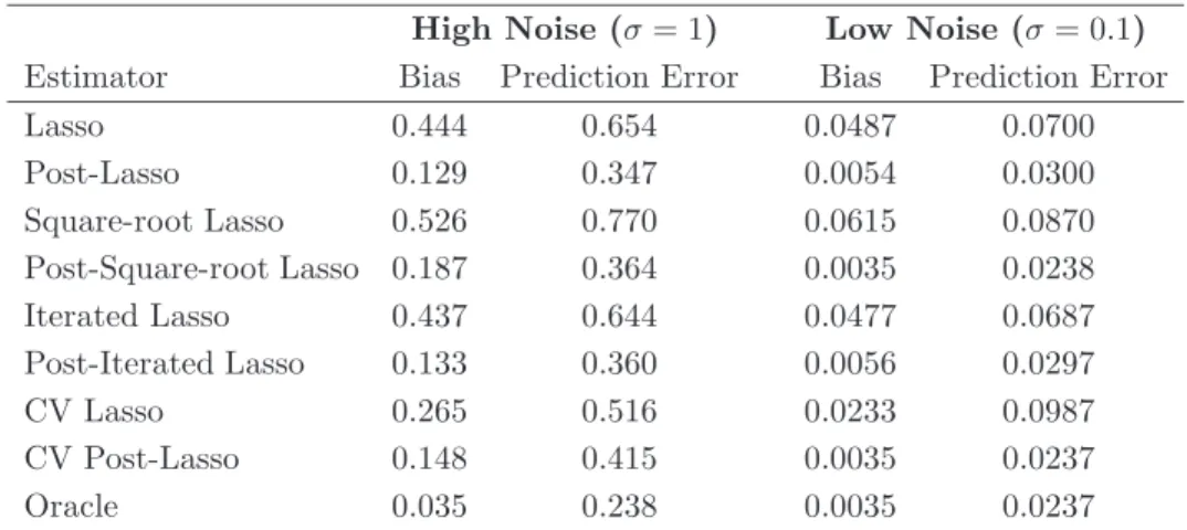
We consider infeasible Lasso and Post-Lasso estimators, feasible Lasso and Post-Lasso esti-mators described in the previous section, all with X-dependent penalty levels, as well as (5-fold) cross-validated (CV) Lasso and Post-Lasso. We summarize results on estimation performance in Table 2 which records for each estimator ¯β the norm of the bias kE[ ¯β −β0]k and also the empirical risk_{E[(x′

i( ¯β−β0))2]}1/2 for recovering the regression function. In this design, infeasible Lasso, Square-root Lasso, and Iterated Lasso exhibit substantial bias toward zero. This bias is somewhat alleviated by choosing the penalty-level via cross-validation, though the

remaining bias is still substantial. It is also apparent that, as intuition and theory would sug-gest, the post-penalized estimators remove a large portion of this shrinkage bias. We see that among the feasible estimators, the best performing methods are the Post-Square-root Lasso and Post-Iterated Lasso. Interestingly, cross-validation also produces a Post-Lasso estimator that performs nearly as well, although the procedure is much more expensive computationally. The Post-Lasso estimators perform better than Lasso estimators primarily due to a much lower shrinkage bias which is beneficial in the design considered.

High Noise (σ= 1) Low Noise (σ= 0.1)

Estimator Bias Prediction Error Bias Prediction Error

Lasso 0.444 0.654 0.0487 0.0700 Post-Lasso 0.129 0.347 0.0054 0.0300 Square-root Lasso 0.526 0.770 0.0615 0.0870 Post-Square-root Lasso 0.187 0.364 0.0035 0.0238 Iterated Lasso 0.437 0.644 0.0477 0.0687 Post-Iterated Lasso 0.133 0.360 0.0056 0.0297 CV Lasso 0.265 0.516 0.0233 0.0987 CV Post-Lasso 0.148 0.415 0.0035 0.0237 Oracle 0.035 0.238 0.0035 0.0237

Table 2. The table displays the mean bias and the mean prediction error. The average number of components selected by Lasso was 5.18 in the high noise case and 6.44 in the low noise case. In the case of CV Lasso, the average size of the model was 29.6 in the high noise case and 10.0 in the low noise case. Finally, the CV Post-Lasso selected models with average size of 7.1 in the high noise case and 6.0 in the low noise case.

5. Inference on Structural Effects with High-Dimensional Instruments 5.1. Methods and Theoretical Results. In this section, we consider the linear instrumental variable (IV) model with many instruments. Consider the Gaussian simultaneous equation model: y1i=y2iα1+w′_iα2+ζi, (5.35) y2i=f(zi) +vi, (5.36) ζi vi ! |zi ∼N 0, σ2 ζ σζv σζv σv2 !! . (5.37)

Here y1i is the response variable, y2i is the endogenous variable, wi is a kw-vector of control variables,zi= (u′_i, w_i′)′ is a vector of instrumental variables (IV), and (ζi, vi) are disturbances that are independent of zi. The function f(zi) = E[y2i|zi], the optimal instrument, is an unknown, potentially complicated function of the elementary instruments zi. The main pa-rameter of interest is the coefficient on y2i, whose true value is α1. We treat {zi} as fixed throughout.

Based on these elementary instruments, we create a high-dimensional vector of technical instruments,xi =P(zi), with dimension p possibly much larger than the sample size though restricted via conditions stated below. We then estimate the the optimal instrumentf(zi) by

b

f(zi) =x′_iβ,b (5.38) whereβbis a feasible Lasso or Post-Lasso estimator as formally defined in the previous section. Sparse-methods take advantage of approximate sparsity and ensure that many elements of b

β are zero when p is large. In other words, sparse-methods will select a small subset of the available technical instruments. LetAi = (f(zi), wi′)′ be the ideal instrument vector, and let

b

Ai = (fb(zi), w_i′)′ (5.39) be the estimated instrument vector. Denotingdi= (y2i, wi′)′, we form the feasible IV estimator using the estimated instrument vector as

b α∗=En[Aidb ′_i]− 1 En[Aiyb 1i] . (5.40)

The main regularity condition is recorded as follows.

Condition ASIV. In the linear IV model (5.35)-(5.37) with technical instruments xi = P(zi), the following assumptions hold: (i) the parameter values σv, σζ and the eigenvalues

of Qn =En[AiA′_i] are bounded away from zero and from above uniformly in n, (ii) condition ASM holds for (5.36), namely for each i = 1, ..., n, there exists β0 ∈ Rp, such that f(zi) = x′_iβ0+ri, kβ0k6s, {En[r2i]}1/26Kσv

p

s/n, where constant K does not depend on n, (iii) condition SE holds forEn[xix′i], and (iv) s2log2(p∨n) =o(n).

The main inference result is as follows.

Theorem 3 (Asymptotic Normality for IV Estimator Based on Lasso and Post-Lasso). Sup-pose Condition ASIV holds. The IV estimator constructed in (5.40) is √n-consistent and is asymptotically efficient, namely as ngrows:

(σ2_ζQ−1_n )−1/2√n(αb∗−α) =N(0, I) +oP(1),

and the result also holds withQn replaced byQbn=En[AbiAb′i]andσ2ζ byσb2ζ =En[(y1i−Ab′iαb∗)2].

Comment 5.1. The theorem shows that the IV estimator based on estimating the first-stage with Lasso or Post-Lasso is asymptotically as efficient as the infeasible optimal IV estimator that usesAi and thus achieves the semi-parametric efficiency bound of Chamberlain (1987). Belloni, Chernozhukov, and Hansen (2010) show that the result continues to hold when other sparse methods are used to estimate the optimal instruments. The sufficient conditions for showing the IV estimator obtained using sparse-methods to estimate the optimal instruments is asymptotically efficient include a set of technical conditions and the following key growth condition: s2_log2_(p

∨n) = o(n). This rate condition requires the optimal instruments to be sufficiently smooth so that a relatively small number of series terms can be used to approximate

them well. This smoothness ensures that the impact of instrument estimation on the IV estima-tor is asymptotically negligible. The rate conditions2_log2

(p_∨n) =o(n) can be substantive and cannot be substantially weakened for the full-sample IV estimator considered above. However, we can replace this condition with the weaker condition thatslog(p∨n) =o(n) by employing a sample splitting method from the many instruments literature (Angrist and Krueger 1995) as established in Belloni, Chernozhukov, and Hansen (2010) and Belloni, Chen, Chernozhukov, and Hansen (2010). Moreover, Belloni, Chen, Chernozhukov, and Hansen (2010) show that the result of the theorem, with some appropriate modifications, continues to apply under het-eroscedasticity though the estimator does not necessarily attain the semi-parametric efficiency bound. In order to achieve full efficiency allowing for heteroscedasticity, we would need to estimate the conditional variance of the structural disturbances in the second stage equation. In principle, this estimation could be done using sparse methods.

5.2. Weak Identification Robust Inference with Very Many Instruments. Consider the simultaneous equation model:

y1i=y2iα1+w_i′α2+ζi, ζi|zi ∼N 0, σ2ζ

, (5.41)

wherey1i is the response variable, y2i is the endogenous variable, wi is akw-vector of control variables,zi= (u′i, wi′)′ is a vector of instrumental variables (IV), andζi is a disturbance that is independent ofzi. We treat {zi} as fixed throughout.

We would like to use a high-dimensional vector xi = P(zi) of technical instruments for inference that is robust to weak identification. We propose a method for inference based on inverting pointwise tests performed using a sup-score statistic defined below. The procedure is similar in spirit to Anderson and Rubin (1949) and Staiger and Stock (1997) but uses a very different statistics that is well-suited to cases with very many instruments.

In order to formulate the sup-score statistic, we first partial-out the effect of controlswi on the key variables. For ann-vector_{ui, i= 1, ..., n}, define ˜ui =ui−wi′En[wiwi′]−1En[wiui], i.e. the residuals left after regressing this vector on _{wi, i= 1, ..., n}. Hence ˜y1i, ˜y2i, and ˜xij are residuals obtained by partialling out controls. Also, let ˜xi = (˜xi1, ...,x˜ip)′. In this formulation, we omit elements ofwifrom ˜xij since they are eliminated by partialling out. We then normalize without loss of generality

En[˜x2_ij] = 1, j = 1, ..., p. (5.42) The sup-score statistic for testing the hypothesisα1 =atakes the form:

Λa= max 16j6p |nEn[(˜y1i−y˜2ia)˜xij]| q En[(˜y1i−y˜2ia)2x˜2_ij] .

If the hypothesisα1 =ais true, then the critical value for achieving level γ is Λ(1−γ|W, X) = 1−γ−quantile of max 16j6p |nEn[˜gix˜ij]| q En[˜gi2x˜2ij] |W, X (5.43)

whereW = [w1, ..., wn]′,X= [x1, ..., xn]′, andg1, ..., gn are i.i.d. N(0,1) variables independent ofW and X; ˜gi denotes the residuals left after projecting{gi} on {wi} as defined above. We can approximate the critical value Λ(1₋γ_|W, X) by simulation conditional on X and W. It is also possible to use a simple asymptotic bound on this critical value of the form

Λ(1₋γ) :=c√nΦ−1(1₋γ/2p)_≤cp2nlog(2p/γ), (5.44) forc >1. The finite-sample (1−γ) – confidence region for α1 is then given by

C:={a∈R: Λa6Λ(1−γ|W, X)},

while a large sample (1₋γ) – confidence region is given by_C′ _{:={a∈R: Λ}

a6Λ(1−γ)}. The main regularity condition is recorded as follows.

Condition HDIV. Suppose the linear IV model (5.41) holds. Consider the p-vector of instruments xi =P(zi), i= 1, ..., n, such that (logp)/n→ 0. Suppose further that the

follow-ing assumptions hold uniformly in n: (i) the parameter value σζ is bounded away from zero

and from above, (ii) the dimension of wi is bounded and the eigenvalues of the Gram matrix

En[wiw′i] are bounded away from zero, (iii) kwik6K and |x˜ij|6K for all 16i6n and all 16j6p, where K is a constant, independent of n.

The main inference result is as follows.

Theorem 4 (Valid Inference based on the Sup-Score Statistic). (1) Suppose the linear IV model (5.41) holds. Then P(α1 ∈ C) = 1−γ. (2) Suppose further that condition HDIV holds,

then P(α1 ∈ C′)>1−γ−o(1). (3) Moreover, if a is such that that max 16j6p |a−α1|√n|En[˜y2ix˜ij]|/√logp σζ+|a−α1| q En[˜y22ix˜ 2 ij] → ∞,

then P(a∈ C) =o(1) andP(a∈ C′_{) =o(1).}

Comment 5.2. The theorem shows that the confidence regions _C and _C′ constructed above have finite-sample and large sample validity, respectively. Moreover, the probability of includ-ing a false pointa in either C or C′ _{tends to zero as long as a is sufficiently distant from α}

1 and instruments are not too weak. In particular, if there is a strong instrument, the confi-dence regions will eventually exclude pointsathat are further thanp(logp)/naway fromα1. Moreover, if there are instruments whose correlation with the endogenous variable is of greater order than p(logp)/n, then the confidence regions will asymptotically be bounded. Finally, note that a nice feature of the construction is that it provides provably valid confidence regions and does not require computation of some combinatorial quantities, in sharp contrast to other recent proposals for inference, e.g. Gautier and Tsybakov (2011). Lastly, we note that it is not difficult to generalize the results to allow for an increasing number of controls wi under suitable technical conditions that restrict the number of controls and their envelope in relation to the sample size. Here we did not consider this possibility in order to highlight the impact of

very many instruments more clearly. The result (2) extends to non-Gaussian, heteroscedastic cases; we refer to Belloni, Chen, Chernozhukov, and Hansen (2010) for relevant details. Comment 5.3 (Inverse Lasso Interpretation). The construction of confidence regions above can be given the followingInverse Lasso interpretation. Let

b

βa= arg min

β∈RpEn[(˜y1i−a˜y2i)−x˜ ′ ijβ]2+ λ n p X j=1

|βj|γaj, γaj=qEn[(˜y1i−y˜2ia)2x˜2_ij]. If λ = 2Λ(1₋γ_|W, X), then _C is equivalent to the region _{a_∈ R : βba = 0}. If λ= 2Λ(1− γ), then _C′ _{is equivalent to the region {a ∈ R : βb}

a = 0}. In words, to construct these confidence regions, we collect all potential values of the structural parameter, where the Lasso regression of the potential structural disturbance on the instruments yields zero coefficients on the instruments. This idea is akin to the Inverse Quantile Regression and Inverse Least Squares ideas in Chernozhukov and Hansen (2008a) and Chernozhukov and Hansen (2008b).

5.3. Monte Carlo Example: Instrumental Variable Model. The theoretical results pre-sented in the previous sections suggest that using Lasso to aid in fitting the first-stage regression should result in IV estimators with good estimation and inference properties. In this section, we provide simulation evidence on these properties of IV estimators using iterated Lasso to select instrumental variables for a second-stage estimator. We also considered Square-root Lasso for variable selection. The results were similar to those for iterated Lasso, so we report only the iterated Lasso results.

Our simulations are based on a simple instrumental variables model of the form y1i =αy2i+ζi y2i =x′_iΠ +vi ζi vi ! |xi∼N 0, σ2 ζ σζv σζv σv2 !! i.i.d.,

whereα= 1 is the parameter of interest, andxi= (xi1, ..., xi100)′∼N(0,ΣX) is the instrument vector with E[x2_ih] = σ2_x and Corr(xih, xij) = .5|j−h|. In all simulations, we set σζ2 = 1 and σ2

x= 1. We also use Corr(ζ, v) = .3.

We consider several different settings for the other parameters. We provide simulation results for sample sizes,n, of 100 and 500. In one simulation design, we set Π = 0 andσ2

v = 1. In this case, the instruments have no information about the endogenous variable, soα is unidentified. We refer to this as the “No Signal” design. In the remaining cases, we use an “exponential” design for the first stage coefficients, Π, that sets the coefficient onxih=.7h−1forh= 1, ...,100 to provide an example of Lasso’s performance in settings where the instruments are informative. This model is approximately sparse, since the majority of explanatory power is contained in the first few instruments, and obeys the regularity conditions put forward above. We consider values ofσ2

v which are chosen to benchmark three different strengths of instruments. The three values ofσ2

v are found as σv2= n Π′Σ_ZΠ

For each setting of the simulation parameter values, we report results from several estimation procedures. A simple possibility when presented with p < n instrumental variables is to just estimate the model using 2SLS and all of the available instruments. It is well-known that this will result in poor-finite sample properties unless there are many more observations than instruments; see, for example, Bekker (1994). Fuller’s (1977) estimator (FULL)10 is robust to many instruments as long as the presence of many instruments is accounted for when constructing standard errors andp < n; see Bekker (1994) and Hansen, Hausman, and Newey (2008) for example. We report results for these estimators in rows labeled 2SLS(All) and FULL(All) respectively.11 _{In addition, we report Fuller and IV estimates based on the set} of instruments selected by Lasso with two different penalty selection methods. IV-Lasso and FULL-Lasso are respectively 2SLS and Fuller using instruments selected by Lasso with penalty obtained using the iterated method outlined in Appendix A. We use an initial estimate of the noise level obtained using the regression of y2 on the instrument that has the highest simple correlation withy2. IV-Lasso-CV and FULL-Lasso-CV are respectively 2SLS and Fuller using instruments selected by Lasso using 10-fold cross-validation to choose the penalty level. We also report inference results based on the Sup-Score test developed in Section 5.2.

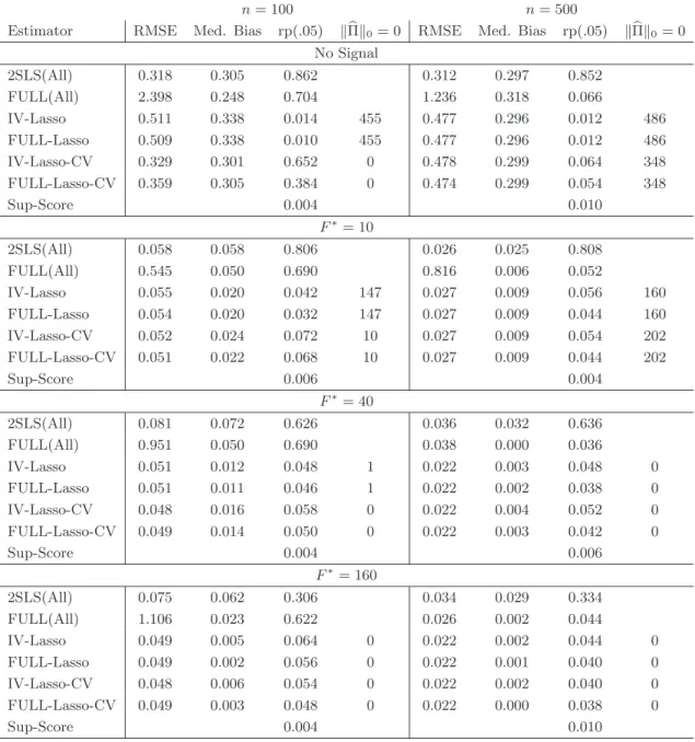
In Table 3, we report root-mean-squared-error (RMSE), median bias (Med. Bias), rejection frequencies for 5% level tests (rp(.05)), and the number of times the Lasso-based procedures select no instruments (_kΠb_k0 = 0). For computing rejection frequencies, we estimate conven-tional 2SLS standard errors for all 2SLS estimators, and the many instrument robust standard errors of Hansen, Hausman, and Newey (2008) for the Fuller estimators. In cases where Lasso selects no instruments, the reported Lasso point estimation properties are based on the feasible procedure that enforces identification by lowering the penalty until one variable is selected. Rejection frequencies in cases where no instruments are selected are based on the feasible procedure that uses conventional IV inference using the selected instruments when this set is non-empty and otherwise uses the Sup-Score test.

The simulation results show that Lasso-based IV estimators is useful in situations with many instruments. As expected, 2SLS(All) does extremely poorly along all dimensions. FULL(All) also performs worse than the Lasso-based estimators in terms of estimator risk (RMSE) in all cases. The Lasso-based procedures do not dominate FULL(All) in terms of median bias, though all of the Lasso-based procedures have smaller median bias than FULL(All) when n = 100 and there is some signal in the instruments and are very similar with n = 500. In terms of size of 5% level tests, we see that the Sup-Score test uniformly controls size as indicated by the theory. IV-Lasso and FULL-Lasso using the iterated penalty selection method also do a very good job controlling size across all of the simulation settings with a worst-case rejection frequency of .064 (with simulation standard error of .01) and the majority of rejection 10_{The Fuller estimator requires a user-specified parameter. We set this parameter equal to one which produces} a higher-order unbiased estimator. See Hahn, Hausman, and Kuersteiner (2004) for additional discussion.

11_{All models include an intercept. Withn= 100, we randomly select 98 instruments to use for 2SLS(All)} and FULL(All).

frequencies below .05. Interestingly, when there is no signal in the instrument, the Lasso-based estimators using penalty selected by CV have substantial size-distortions whenn= 100 which is due to the CV penalty being small enough that instruments are still selected despite there being no signal. The iterated penalty is such that, at least approximately, only instruments whose coefficients are outside of a√nneighborhood of 0 are selected and thus overselection in cases with little signal is guarded against. Despite the problem with using CV when there is no signal, it is worth noting that the Lasso-based procedures with CV penalty produce tests with approximately correct size in all other parameter settings.

To further examine the properties of the inference procedures that appear to give small size distortions, we plot the power curves of 5% level tests using the Sup-Score test and IV-Lasso with the iterated and CV penalty choices with n = 100 in Figure 2.12 We see that both the Sup-Score test and IV-Lasso using the iterated procedure augmented with Sup-Score test when no instruments are selected appear to uniformly control size and have some power against alternatives when the model is identified. It is also clear that of these two procedures, the IV-Lasso has substantially more power than the Sup-Score test. The figures also show that IV-Lasso with iterated penalty has almost as much power as IV-Lasso using the CV penalty while avoiding the substantial size distortion and spurious power produced by using CV when there is no signal.

Overall, the simulation results are favorable to the based IV methods. The Lasso-based estimators dominate the other estimators considered Lasso-based on RMSE and have relatively small finite sample biases. The Lasso-based procedures also do a good job in producing tests with size close to the nominal level. There is some evidence that the Fuller-Lasso may do better than 2SLS-Lasso in terms of testing performance though these procedures are very similar in the designs considered. It also seems that tests based on IV-Lasso using the iterated penalty selection rule may perform better than tests based on IV-Lasso using cross-validation to choose the Lasso penalty levels, especially when there is little explanatory power in the instruments.

6. Inference on Treatment and Structural Effects Conditional on Observables

6.1. Methods and Theoretical Results. We consider the following partially linear model, y1i =diα0+g(zi) +ζi, (6.45) di =m(zi) +vi, (6.46) ζi vi ! |zi ∼N 0, σ2 ζ 0 0 σ2 v !! (6.47) wheredi is a policy/treament variable whose impact we would like to infer, and zi represents confounding factors on which we need to condition. This model is of interest in our international

12_{The power curves in the}

Instrumental Variables Model Simulation Results

n= 100 n= 500

Estimator RMSE Med. Bias rp(.05) kΠkb 0= 0 RMSE Med. Bias rp(.05) kΠkb 0= 0

No Signal 2SLS(All) 0.318 0.305 0.862 0.312 0.297 0.852 FULL(All) 2.398 0.248 0.704 1.236 0.318 0.066 IV-Lasso 0.511 0.338 0.014 455 0.477 0.296 0.012 486 FULL-Lasso 0.509 0.338 0.010 455 0.477 0.296 0.012 486 IV-Lasso-CV 0.329 0.301 0.652 0 0.478 0.299 0.064 348 FULL-Lasso-CV 0.359 0.305 0.384 0 0.474 0.299 0.054 348 Sup-Score 0.004 0.010 F∗_{= 10} 2SLS(All) 0.058 0.058 0.806 0.026 0.025 0.808 FULL(All) 0.545 0.050 0.690 0.816 0.006 0.052 IV-Lasso 0.055 0.020 0.042 147 0.027 0.009 0.056 160 FULL-Lasso 0.054 0.020 0.032 147 0.027 0.009 0.044 160 IV-Lasso-CV 0.052 0.024 0.072 10 0.027 0.009 0.054 202 FULL-Lasso-CV 0.051 0.022 0.068 10 0.027 0.009 0.044 202 Sup-Score 0.006 0.004 F∗_{= 40} 2SLS(All) 0.081 0.072 0.626 0.036 0.032 0.636 FULL(All) 0.951 0.050 0.690 0.038 0.000 0.036 IV-Lasso 0.051 0.012 0.048 1 0.022 0.003 0.048 0 FULL-Lasso 0.051 0.011 0.046 1 0.022 0.002 0.038 0 IV-Lasso-CV 0.048 0.016 0.058 0 0.022 0.004 0.052 0 FULL-Lasso-CV 0.049 0.014 0.050 0 0.022 0.003 0.042 0 Sup-Score 0.004 0.006 F∗_{= 160} 2SLS(All) 0.075 0.062 0.306 0.034 0.029 0.334 FULL(All) 1.106 0.023 0.622 0.026 0.002 0.044 IV-Lasso 0.049 0.005 0.064 0 0.022 0.002 0.044 0 FULL-Lasso 0.049 0.002 0.056 0 0.022 0.001 0.040 0 IV-Lasso-CV 0.048 0.006 0.054 0 0.022 0.002 0.040 0 FULL-Lasso-CV 0.049 0.003 0.048 0 0.022 0.000 0.038 0 Sup-Score 0.004 0.010

Table 3. Results are based on 500 simulation replications. F∗ _{measures the strength of}

the instruments as outlined in the text. We report root-mean-square-error (RMSE), median bias (Med. Bias), rejection frequency for 5% level tests (rp(.05)), and the number of times the Lasso-based procedures select no instruments (kΠkb 0= 0). Further details are provided in

the text.

growth example discussed in the next section as well as in many empirical studies (Heckman, LaLonde, and Smith 1999, Imbens 2004). The confounding factors affect the policy variable viam(zi). We assume thatm(zi) andg(zi) each admit an approximately sparse form and use linear combinations of technical control termsxi =P(zi) to approximate them.

0.5 1 1.5 0 0.2 0.4 0.6 0.8 1 n = 100, No Signal 0.5 1 1.5 0 0.2 0.4 0.6 0.8 1 n = 100, F* = 10 0.5 1 1.5 0 0.2 0.4 0.6 0.8 1 n = 100, F* = 40 0.5 1 1.5 0 0.2 0.4 0.6 0.8 1 n = 100, F* = 160

Sup−Score IV−Lasso: Plug−In IV−Lasso: CV

Figure 2. Power curves for Sup-Score test, IV-Lasso with Iterated penalty, and IV-Lasso with penalty selected by 10-Fold Cross-Validation from IV simulation with 100 observations.

There are at least three obvious strategies for inference:

(i) Estimate α0 by applying a Feasible Lasso method to model (6.45) without penalizing α0,

(ii) Estimateα0 by applying a Post-Lasso method to model (6.45) without penalizing α0, (iii) Estimate α0 by applying an Indirect Post-Lasso where α0 is estimated by running standard least squares regression ofy ondand control terms selected in a preliminary Feasible Lasso regression of di onxi in (6.46).

Note that it is most natural not to penalize α0 since the goal is to quantify the impact of di. (The previous rate results derived in Theorems 1 and 2 for the regression function extend to the case where the coefficients on a fixed number of variables are not penalized.) In what follows, we shall refer to options (i), (ii), and (iii) respectively as Lasso, Post-Lasso, and Indirect Post-Lasso.

Regarding inference, “intuition” suggests that ifg can be estimated at faster than then1/4 rate then any of (i)-(iii) could be√n-consistent and asymptotically normal. It turns out that

this “intuition” is often correct for options (ii) and (iii) but is wrong for option (i). Indeed, it is possible to show that under rather strong regularity conditions that

(σ_ζ2[Env2_i]−1)−1/2√n(¯α−α0) =N(0,1) +oP(1), (6.48) whereσ2

ζ[Env 2

i]−1 is the semi-parametric efficiency bound for estimatingα0, for ¯αdenoting the estimators (ii) or (iii) above. Unfortunately, the distributional result (6.48) is not very robust to modest violations of regularity conditions and may provide a poor approximation to the finite-sample distributions of the estimators forα0. The reason is that Lasso applied to (6.45) may miss important terms relating di to zi through m(zi) and thus suffer from substantial omitted variables bias. On the other hand, Lasso applied only to (6.46), even if successful in selecting adequate controls for the relationship betweendi andzi, may miss important terms in g(zi) and thus be highly inefficient. We illustrate this lack of robustness through a simulation experiment reported below.

Instead of using Lasso, Post-Lasso, or Indirect Post-Lasso, we advocate a “double-Post-Lasso” method. To define this estimator, we write the reduced form corresponding to (6.45)-(6.46):

y1i =α0m(zi) +g(zi) +α0vi+ζi, (6.49)

di =m(zi) +vi. (6.50)

Now we have two equations and hence can apply Lasso methods to each equation to select control terms. That is, we run Lasso regression of y1i on xi =P(zi) and Lasso regression of di on xi = P(zi). Then we can run least squares of y1i on di and the union of the controls selected in each equation to estimate and perform inference onα0. By using this procedure we increase the chances for successfully recovering terms that approximate the key control term m(zi), which results in improved robustness properties. Indeed, the resulting procedure is considerably more robust in computational experiments and requires much weaker regularity conditions than the obvious strategies outlined above.

Now we formally define the double-Post-Lasso estimator. Let Ib1 = support(bβ1) denote the control terms selected by a feasible Lasso estimator βb1 computed using data (yi, xi) = (di, xi), i = 1, ..., n. Let Ib2 = support(βb2) denote the control terms selected by a feasible Lasso estimatorβb2 computed using data (yi, xi) = (y1i, xi), i= 1, ..., n. The double-Post-Lasso estimator ˇαofα0 is defined as the least squares estimator obtained by regressingy1i ondi and the selected control termsxij withj ∈Ib⊇Ib1∪Ib2:

(ˇα,β) = argminˇ α∈R,β∈Rp{En

[(y1i−diα−x′iβ)2] : βj = 0,∀j6∈Ib}.

The setIbcan contain other variables with namesIb3 that the analyst may think are important for ensuring robustness. Thus,Ib=Ib1∪Ib2∪Ib3; let bs=|Ib|andsbj =|Ibj|forj= 1,2,3.

Condition ASTE.(i) The data (y1i, di, zi), i= 1, ..., n, obeys model (6.45)-(6.47) for each n, andxi=P(zi) is a dictionary of transformations ofzi. (ii) The parameter valuesσ2v andσζ2