Learning Pose Estimation for UAV Autonomous Navigation and
Landing Using Visual-Inertial Sensor Data
Francesca Baldini
1, Animashree Anandkumar
1, and Richard M. Murray
1Abstract— In this work, we propose a robust network-in-the-loop control system that allows an Unmanned-Aerial-Vehicles to navigate and land autonomously on a desired target. To estimate the global pose of the aerial vehicle, we develop a deep neural network ar-chitecture for visual-inertial odometry, which provides a robust alternative to traditional techniques for au-tonomous navigation of Unmanned-Aerial-Vehicles. We first provide experimental results on the accuracy of the estimation by comparing the prediction of our model to traditional visual-inertial approaches on the publicly available EuRoC MAV dataset. The results indicate a clear improvement in the accuracy of the pose estima-tion up to 25% against the baseline. Second, we use Airsim, a simulator available as a plugin for Unreal Engine, to create new datasets of photorealistic images and inertial measurement to train and test our model. We finally integrate the proposed architecture for global localization with the Airsim closed-loop control system, and we provide simulation results for the autonomous landing of the aerial vehicle.
I. INTRODUCTION
Unmanned-Aerial-Vehicles (UAVs) can provide signif-icant support for many applications, such as rescue operations, environmental monitoring, package delivery, and surveillance. To guarantee a high safety level in the UAV operation, it is crucial to have continuous monitoring of the state of the vehicle. Currently, the most standard techniques deployed for pose estimation are Visual-Inertial Odometry (VIO) [1, 2] and Simultane-ous Localization and Mapping (SLAM) [3–5]. However, these methods have been proven not to be robust to challenging conditions, such as low-texture or low-light environments, noise and blur, camera occlusion, dynamic objects in the scene, and camera calibrations errors [1, 6, 7].
The advent of deep-learning techniques has led to the development of a wide variety of improvements in the computer vision algorithms [8]. Data-driven approaches have shown outstanding performance in various applica-tions. Even if learning an estimator from data requires a significant amount of labels, their robustness to illumi-nation changes, noise, and blur compared to traditional VIO and SLAM methods, makes learning algorithm more attractive for vision-based applications. VIO/SLAM methods tracks hand-engineered selected points along
F.Baldini is supported in part by Darpa PAI grant HR0011-18-9-0035. A. Anandkumar is supported in part by Darpa PAI grant HR0011-18-9-0035, Bren Endowed Chair, Microsoft Faculty Fellowship, Google Faculty Award, Adobe Grant,
1California Institute of Tecnology, Pasadena CA 91125, USA
images to perform localization. In the presence of noise and blurs, these features are not easy to recognize and track. In contrast, DNNs learn which features are more meaningful for localization tasks. By eliminating the need for feature selection, DNNs provide robust alter-native solutions to autonomous navigation [8, 9].
a) Contribution: In this paper, we propose a robust end-to-end learning control system for UAV autonomous navigation and landing. We train the model to learn the function that relates raw images and inertial data to 6-DOF global poses. We assess the performance of the model by comparing it to well known baseline VIO on the public available EuRoC MAV dataset. The results show that our method significantly outperforms the state-of-the-art visual odometry estimation, improving the accu-racy of the estimation up to 25% against the baseline.
In order to use the proposed algorithm for real-time autonomous navigation and landing, we train and test our model on new datasets generated using Airsim [10], a flight simulator available as a plugin for Unreal Engine. This tool provides photo-realistically rendered RGB images that minimize the gap between reality and simulation. We used the steady-state covariance from a Kalman Filter (KF) as a quality measure for the proposed algorithm. Based on the experimental results, we found an empirical bound for the ML estimation of 10 cm. Experimental results show that our algorithm tracks the robot position with a median error, in the worse case, no larger than 30 cm compared to the KF estimation. As an additional comparison, we implemented the ORB-SLAM [11] algorithm on the same AirSim datasets. However, given noises and blurs input images, the al-gorithm failed the position tracking in all the datasets collected. Hand-engineered features are hard to track in the presence of noise. By learning features that are more meaningful for localization tasks, our algorithm provides a more robust UAV tracking method compared to traditional approaches.
Finally, we integrate our architecture with a position-based control scheme to perform autonomous navigation and landing. We validate the data-driven closed-loop flight control system on the Downtown environment simulated in Airsim [10]. We show through real-time simulations that, during the final landing phase, when high positioning precision is required, the closed-loop neural-based control system can navigate and land the UAV on the designed target with less than 10 cm of errors.
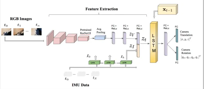
Fig. 1. The architecture of the proposed neural-network for global pose estimation with sensor fusion consisting of visual and inertial encoders, feature concatenations, temporal modeling, and pose regression. The CNN determines the most discriminative visual featureszV while a small LSTM transforms windows of inertial measurements into a single inertial feature vectorzI. Finally, the visual and inertial feature vectors are concatenated into a single representationzt. A core LSTM takes in input the feature vectorztand the previous estimatext−1and outputs the current estimate of the pose (translation and rotation).
b) Previous Works: Traditional localization-based approaches to autonomous drone navigation rely on computer vision algorithms supplemented by sensors, including Global Positioning Systems (GPS) and Inertial Measurement Units (IMUs), for pose estimation [2, 12– 14]. A traditional pipeline for VIO and SLAM typically consists of camera calibration, followed by feature de-tection and tracking, outlier rejection, motion, and scale estimation, optimization back-end, and local optimization (Bundle Adjustment). Visual Servoing methods use the tracked features as inputs to a control law that directs the robot into a desired pose [6, 15, 16]. However, en-vironmental noise and the presence of dynamic objects can negatively affect the tracking process and reduce the estimation accuracy. Overall, VIO systems demand heavy computation due to image processing and sensor fusion. When the vehicle flies at a very high speed, there is a need to track the position of the robot at a high rate. To this end, [17] presented a real-time simulation tool that interconnects with a real UAV. Finally, they use synthetic images and real IMU data for visual-inertial-odometry. Carlone et al. [18] have proposed a visual feature selection scheme for visual-inertial-navigation. A cardinality constraint is imposed on the selected mea-surements to control the computational cost of solving the pose estimation problem.
The advent of deep learning techniques has created new benchmarks in almost all areas of computer vision. Recently, CNN architectures for pose estimation have been capturing lots of interests in machine learning and control community [19–22]. PoseNet [23] has been the first approach to utilize CNNs to address the metric localization problem. In order to provide a more robust approach to balance both the translational and rotational
components in the loss term, they replace the regularizer term with learnable parameters. Other architectures [19, 20, 24–26] have been additionally deployed to esti-mate the incremental motion of the camera using only sequential camera images or a combination of visual and inertial data [20].
II. PRELIMINARIES
a) Estimation Problem: Given the actual state of the robot xt = [xt,yt,zt,qwt,qxt,qyt,qzt]
T
∈ R7, we train the neural network to regress its estimate xˆt=
[ ˆxt, ˆyt, ˆzt, ˆqwt, ˆqxt, ˆqyt, ˆqzt]
T
∈R7 from continuous stream of images and inertial data.
The inputs to our model are photorealistic RGB images
IVt and IMU measurements yt={IIt,IVt}, where the
vec-tor IIt=[τt,axt,ayt,azt,ωxt,ωyt,ωzt]
T ∈RN×7, τ
t denotes
the timestamp of the inertial measurement,at is linear
acceleration, ωt is angular velocity, and N is defined by
the number of inertial measurements observed between two camera timestamps tand t+1.
The estimation problem can be summarized as follows: produce an estimatexˆtthat is as close as possible to the
actual state xt of the robot based on the measurement
yt.
b) Control Problem: We make the assumption that the target positionxposd es=[xd es,yd es,zd es]T is know.
After the controller receives the reference posi-tion of the target xd espos, the desired velocities xveld es =
[ud es,vd es,wd es]T are computed based on the rate of
change of position set points, i.e.,xveld es=x˙posd es.
Subsequently, we use these velocity references xveld es
along with the position reference xd espos to compute the final throttle and attitude angle commands ucom =
[Fzd es,phid es,θd es,ψd es]T that are fed back into the
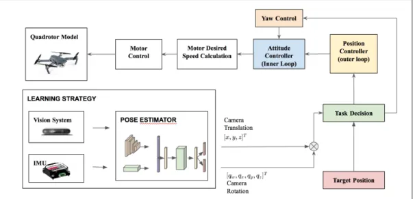
Fig. 2. High-level illustration of the proposed data-driven GNC model. The neural network estimates the 6 DOF of the vehicle. The predicted pose is then used together with the desired state vector to define the velocity command for the low-level controller.
Given the target pose coordinate, we simulate a control law forucomdepending only on xd espos, ˙xd espos such thatxt→ xd espos and (vt,ωt)→0.
Fig. 2 shows an overview of the system architecture for our neural estimator algorithm.
III. ARCHITECTURE
Fig. 1 shows the proposed visual-inertial learning architecture. We assume to have in input synchronized measurements from the vision and inertial sensors (i.e., they start recording at the same time, and the inertial sensors frequency of measurements is a multiple of the camera frame capturing frequency).
A. Network Architecture
The primary goal of our model is to estimate the global pose of the robot by minimizing the geometry consistency loss function described in III-B. Like ViNet [20], our architecture includes a convolutional neural network (CNN) that takes in inputs streams of images, a small LSTM that integrates the IMU measurements between consecutive images, and a core LSTM followed by fully-connected layers that are trained to regress the 6-DOF of the vehicle.
Note that, in contrast to ViNet [20], which is trained to estimate the relative transformation between 2 consec-utive frames of images and the transformation matrix with respect to a reference image, we aim to provide a global representation of the state estimate,i.e., global position and orientation of the robot.
In summary, the neural network can be seen as a sensor which processes raw data at each timestamp and produces an observation vector yt.
a) CNN-based feature extractor: To learn effective features from images that are suitable for the global pose estimation problem, we build upon the ResNet18 architecture, pre-trained on the ImageNet dataset, with
the following modifications. The structure is similar to the ResNet18 truncated before the last average pooling layer. Each of the convolutions is followed by batch normalization and Rectified Linear Unit (ReLU). We replace the average pooling with global average pooling and subsequently add two inner-product layers which output a visual feature vector representation zVt.
b) LSTM for inertial feature extraction: IMU data is generally available at a frequency that is an order of magnitude higher (e.g., 100−200H z) than visual data (e.g., 10−20H z). We then process windows of IMU measurements (representing robot motions) between con-secutive images timestamp using a small Long Short-Term Memory (LSTM) (two-layer bi-directional) as iner-tial feature encoder to recover the latent connection be-tween motion characteristics and data features. LSTMs can exploit these temporal dependencies by maintaining hidden states throughout the window.
c) Intermediate fully-connected layer: The final hidden-layer of the LSTM outputs an inertial feature vector zIt representation that is concatenated with the
visual feature vector representationzVt and fused into a
single feature vector zt=f(zVt,zIt). This vector is then
finally carried over to the core LSTM for sequential modeling.
d) Core LSTM: A core LSTM takes as input the combined feature representation zt and its previous
hidden states ht−1 and models the dynamics and the
connections between sequences of features, where ht= f(zt,ht−1). The use of the LSTM module allows for the
rapid deployment of visual-inertial pose tracking. They can maintain the memory of the hidden states over time and have feedback loops among them. In this way, they enable their hidden state to be related to the previous one and allows them to learn the connection between the previous input and states in the sequence.
e) Fully-connected layer: The output of the LSTM is carried into a fully-connected layer which serves as odometry estimation. The first inner-product layer is of dimension 1024, and the following two are of dimensions 3 and 4 for regressing the translation x and rotation q
as quaternions. In synthesis, the fully connected layer maps the features vector zt representation into a pose
vector as follows: xt=LST M(zt,ht−1). B. Learning and Inference
We train the entire network through loss gradient backpropagation. We use Stochastic Gradient Descent (SGD) to update the weights of the network. To regress the pose of the vehicle, we compute the Euclidean loss between the estimated pose and the ground truth. We adopt Adam [27] optimizer to minimize this loss function, starting with an initial rate of 10−4.
a) Loss Function: We predict the position and ori-entation of the robot following [28], with the following modification. In our loss function, we introduce an addi-tional constraint that penalizes the L1norm in addition to the L2 Euclidean norm. Let x=[x,y,z]∈R3 and q=
[qw,qx,qy,qz]∈R4 denote the ground-truth translation
and rotation vector respectively, and xˆ and qˆ their estimates.
The resulting loss function is as follows:
Lβ(I)=Lx(I)+βLq(I) (1) where Lx(I) = kxˆ −xkL2+γkxˆ−xkL1 and Lq(I) = ° ° °qˆ− q kqk ° ° °L 2+ γ°° °qˆ− q qk ° ° °L 1
represents the translation and the rotation loss, β is a scale factor that balances the weights of position and orientation, which are expressed in different units, and γ is a coefficient introduced to balance the two Euclidean norms. However, as shown in in [28],βrequires significant tuning to get consistent re-sults. To avoid this problem, we replaceβby introducing learnable parameters.
The final loss function implemented in the paper is as follows: Lσ(I)=Lx(I) exp (−sˆx)+sˆx+Lq(I) exp ¡ −sˆq ¢ +sˆq (2)
where ˆs:=log ˆσ2is the learnable variable. Note that each
variable acts as a weight for the respective component in the loss function.
IV. EXPERIMENTS
All the experiments are carried out on a machine with an Intel Xeon CPU E5-2650 @ 2 GHz processor 192 GB RAM, and NVIDIA TITAN RTX GPU. In this section, we compare results from our proposed architecture to the state-of-the-art for VIO on the EuRoC MAV dataset provided by [29].
We additionally evaluate the performance of our model on a new synthetic dataset created using Airsim, an open-source simulator that simulates the physics of the
UAV and renders photorealistic images. Finally, we inte-grate our model into the Airsim’s closed-loop flight con-trol system, and we demonstrate the UAV’s autonomous landing in the simulated scenario.
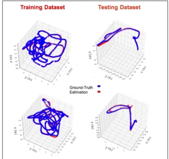
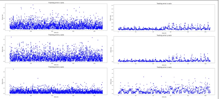
Fig. 3. Sampled 3D trajectories of results on the training and testing sequences
A. Benchmarking
In this section, we evaluate the performances of the proposed network with results from traditional ap-proaches for VIO. We use the publicly available EuRoC MAV Dataset [30] to perform the benchmarking. This dataset consists of eleven visual-inertial challenge se-quences recorded onboard a micro-aerial-vehicle (MAV) flying in an indoor environment. The data available from this dataset consists of stereo monochrome images at 20 Hz, temporally synchronized IMU data at 200 Hz, and ground truth positioning measurements from the Vicon motion capture system.
TABLE I
MEANERROR ONEUROC MAVDATASET
Algorithm V1-01 V1-02 V1-03 V2-01 V2-02 V2-03 This Paper 0.03 0.05 0.10 0.05 0.05 0.08 svomsf [31] 0.39 0.63 x 0.17 0.37 x msckf [2] 0.29 0.20 0.67 0.11 0.16 1.13 okvis [32] 0.09 0.18 0.2 0.12 0.14 0.14 rovio [1] 0.1 0.10 0,14 0.12 0.14 0.14 vinsmono [7] 0.07 0.10 0.13 0.08 0.08 0.21 vinsmonolc [33] 0.04 0.05 0.12 0.06 0.05 0.09 svogtsam [34] 0.12 0.16 x 0.08 xx x
For quantitative pose evaluation, we compute average root mean square (RMS) translation and rotation error and compare our results to traditional methods [1, 2, 7, 31–34] in terms of root-mean-square-error (RMSE)
performance, as reported in [29]. Table I shows a com-parative analysis of average translation RMSE using the traditional VIO method on the indoor datasets of EuRoC. These datasets have different characteristics, and some are more challenging than others. In all the experiments, we can observe that our method outperforms the base-line.
The translation errors are computed across the entire length of the trajectory and ground truth. The RMSE for regression represents the sample standard deviation of the differences between predicted values and real values
R MSE= s PI i=1( ˆyi−yi) 2 n (3)
where yis the real value and ˆyis the predicted one. Fig. 3 shows an example of the trajectories generated by the model (red) against ground truth (blue) on two of the EuRoC MAV datasets.
B. Simulations
To generate our dataset, we use Airsim [10], an open-source simulator that aims to close the gap between simulation and reality. As a plugin, we can use Airsim in any environment developed for the Unreal Engine (UE). We collect training data in the virtual Downtown
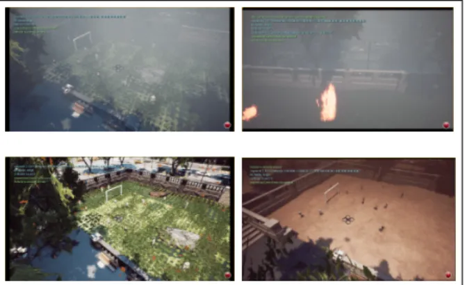
environment retrieved from the Unreal Engine market-place. Fig. 4 shows an example scenario. We create a
Fig. 4. Images sampled from theDowntownsimulated environments used in the paper.
new dataset by driving the vehicle upon a grass field and landing on the surrounding pillars. We split each dataset into two sub-datasets, one for training and the other one for testing. Each flight within the dataset contains timestamped values for the ground-truth 6 DOF pose of the UAV at 100H z, IMU measurements at 100H z, and camera streams (downward-facing) at 10H z. Ground-truth and sensor data are then pre-processed and synchronized.
Hence, we can collect pools of training and test images and IMU data from any phase of flight.
C. Experiment Implementation
We use frames of prerecorded navigation and landing flight in time-order, and results are given in Fig. 3.
In the simulation, the UAV is required to collect training data by flying over the grass field to the top of randomly chosen pillars with constant velocity. The UAV is equipped with a proportional-integral-derivative
(PID) flight controller (FC) that maintains fixed altitude and takes as input the current pose of the vehicle.
We label the recorded frames of the simulator with the corresponding pose measurements from the dataset. The total simulation time is 5h, and we collect images with a step-size of 0.1 seconds. We then split the dataset into two sub-datasets with a ratio of 0.8 and 0.2 as a training and testing set, respectively. We finally downsample the resolution of images to 512×288×3 (RGB) to reduce the computational cost. Each image is normalized to the range [0, 1] dividing by 255.
Fig.??shows a typical trajectory taken by the vehicle (blue), as well as the estimates (red) from our model. It is visually evident that the model tracks the ground-truth trajectory quite accurately.
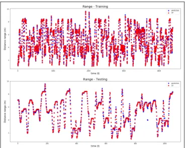
Fig. 5. Range measurements for training and testing dataset
a) Lower bounds from steady-state Kalman filter:
Kalman filters (KF) are the optimal state estimator for systems with the linear process and measurement mod-els. In order to quantify the accuracy of our estimation, we use a worst-case estimation error derived from the steady-state covariance of the KF. This error is used to define a lower bound on the neural network performance. We consider the following discrete-time linear Gaus-sian state-space model:
xt+1=Axt+wt t∈N (4)
yt=Hxk+νt (5)
where xt is the state of the system and yt is the
measurements vector.AandHare matrices of appropri-ate dimensions. The process noise and the measurement noise are distributed according towt≈N(0,Q) and νt≈ N(0,R) respectively, withQ,Rcovariance matrices. This model can be used in a target-tracking context to describe a linear target motion and measurement model.
Fig. 6. Localization RMSE for training and test dataset
We assume that the sensor can measure only the position of the target:
dt= q
(xt−xt)2+(yt−yt)2+(zt−zt)2+d˜t (6)
where ˜dt is the error in the measurement (+/- 1 pixel).
The one step ahead prediction for the performance of a Kalman Filter is given by Pt|t=(I−KtH)Pt|t−1. We
can now formulate Kalman-like recursions for an overall system as follows: Pt+1|t=APt|tAT+Q Kt=Pt|t−1HT ³ HPt|t−1HT+R ´−1 Pt|t=(I−KtH)Pt|t−1 (7)
By performing the proper substitutions, we get:
Pt+1|t=APt|t−1AT−APt|t−1HT ³ HPt|t−1HT+R ´−1 (8) ×HPt|t−1AT+Q
which represents the standard Riccati difference equa-tion associated with the Kalman filter. For k→ ∞, ( 8) has a steady-state algebraic equivalence given by:
P=AP AT−AP HT³HP HT+R´−1HP AT+Q (9)
In general, it is difficult to arrive at a generalized statement that compares Kalman filters with neural networks. The Kalman filter utilizes a linear system for the localization estimates, whereas neural networks localize the vehicle by learning the mapping directly from sensor data to 6-DOF poses. It is then possible to use
the steady-state covariance from a Kalman filter as a quality measure for the proposed estimation algorithms. Based on the experimental results, we found an empirical bound for the ML estimation equal to 10cm.
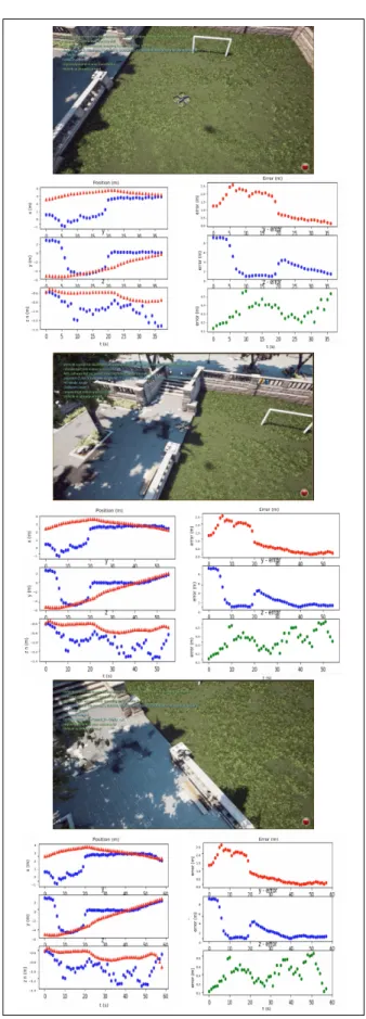
Fig. 7 shows the tracking comparison between the Kalman Filter and ML-based estimation with the ground-truth and measured positions. Fig. 8 reports the RMSE error comparison of both the KF and ML-based with the ground-truth.
Fig. 7. Kalman Filter and ML tracking predictions
Fig. 8. Kalman Filter (blue) and ML (orange) tracking prediction error.
D. UAV Landing
Finally, we simulated the UAV’s autonomous landing by integrating our neural model for pose estimation
with the closed-loop flight control system. Note that our network’s prediction has replaced the default input state estimate for the controller.
We visualize the simulation in Airsim. This tool has a built-in Python API. A non-custom Python script receives state information from our neural-network model and sends it to the Unreal environment by using Airsim API. At the same time, the script captures images and inertial measurements at desired timestamps and labels the captured data with the real state information.
We build a guidance logic that takes in input the current estimate along with the desired target pose and outputs reference velocities to the low-level controller used to control the motors of the vehicle. Fig. 9 shows an overview of the system architecture for autonomous landing.
Fig. 9. Neural Feedback Control Framework
Fig. 10 shows an example of the UAV landing in AirSim. At the starting point, the trained policy shows poor performance, i.e., the model is not able to localize the robot correctly. This occurs because we do not train the model enough around the take-off area, i.e., we did not collect enough labeled data for the training. On the other hand, when the UAV runs into conditions seen during the training, the prediction converges to the actual state. The decision task determines then the new UAV control inputs that guide the system to the desired target.
E. Comparison with traditional methods
Traditional approaches for VIO uses feature descrip-tors such as SIFT, SURF, and ORB [35] to detect "inter-esting"features in the images. In the robotic community, the term feature has a different meaning compared to one used in machine learning. In this case, features are distinguishing points (such as corners and edges) that are easily recognizable in the image.
To be able to perform accurate localization, these algorithms need to recognize and track a significant amount of features through sequences of four or more images. If this condition is not satisfied, the algorithm fails to localize the system.
Now, let us think about what happens when a UAV is required to move with high velocity. Given the low frequency at which the camera sensor operates, we might
Fig. 10. The UAV autonomous landing implemented in AirSim. We use our network’s estimate to update the flight controller. By minimizing the euclidean distance between the current position of the robot and the position of the target, we generate velocity commands that guide the UAV to the landing platform.
Fig. 11. Example of good matches. Features are easily recognizable, and the algorithm is able to match the features correctly in the two images.
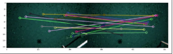
Fig. 12. Example of bad matches. The grass field has not are easily recognizable features. The algorithm tracks points that show some contrast with the background (e.g., some points reflect the light), but the presence of the wind makes this point changing through the image. Hence, the algorithm is not able to match the features correctly.
not be able to have temporally-close sequences of images. Hence, the algorithm is not able to track enough features for more than a couple of images. Consequently, it can either lose track of the position of the system or, in the worse case, not be able to initialize the localization. Ad-ditionally, note that the engineer’s judgment and a long trial and error process decide which kind of features has to be detected and tracked. In other words, algorithms like SIFT, ORB, or pixel counting use non-learned feature descriptors and perform the same way for any given dataset.
Fig. 11 and fig. 12 show an example of feature match-ing with ORB descriptors.
However, this issue does not occur when we deploy DNNs. Learned features are more effective than hand-engineering ones. DNNs, since they are trained rather than programmed, can learn more descriptive and salient features compared to traditional methods and develop better representations for the image data. Convolutional Neural Networks make use of filters (e.g., a matrix of values, called weights) to detect which features are more effective to extract for the given task. Hence, CNNs outperform traditional algorithms like SIFT or ORB.
V. CONCLUSION AND FUTURE WORK
a) Discussion and Limitations: Overall, the ex-perimental results indicate that among the traditional localization algorithms, our method presents the best performance in terms of localization accuracy on the benchmark EuRoC MAV dataset.
One of the advantages of using a neural network over traditional methods is its capability to produce a state estimate in just a single step.
However, as a drawback, supervised-learning networks need to be trained exhaustively in all expected operating
conditions to show outstanding performances. To this end, they require a large amount of training data to ef-fectively samples all those conditions. When the training data are not enough to cover all the expected situation the robot can run into, the network is no longer able to localize the robot, as shown in Fig. 10.
Hence, if even some small changes in the environment occur, the neural network needs to be retrained, and there is the possibility that the architecture may need to change as well.
A. Future Work and preliminary results
a) Learning to Generalize to Dynamic Environments with Meta-Learning: A big challenge for learning-based navigation algorithms is learning to estimate the position of the robot in dynamic environments.
Given that it is impossible to generate training data that cover all possible situations the UAV can encounter, we aim to build a meta-learning/adaptive algorithm that allows the model to predict the 6-DOF pose of the vehicle in unseen conditions.
Fig. 13 shows an example of the perturbedDowntown
environment generated in Airsim. Each environment consists of the same central structure, i.e., a grass field surrounded by pillars, but different weather conditions, materials, lights, etc. are used this time.
b) Loss function for ego-motion consistency: In Fig 10, we can see that, in some cases, the estimated pose is not consistent with the previous estimate. Hence, additional future works will focus on the derivation of a new loss function that incorporates previous motion in-formation to guarantee consistency between continuous streams of data.
B. Conclusion
In this paper, we propose a new network-in-the-loop controller method that allows a UAV to land au-tonomously on a designated target. We train a DNN architecture to the end of the ego-motion estimation, and we finally integrate our estimator in the flight controller. We demonstrate that our model outperforms state-of-the-art methods for visual-inertial estimation on the EuRoC MAV benchmark dataset while providing ex-tra guarantees in robustness and safety compared to geometric-based VIO algorithms. We finally show that the proposed data-driven closed-loop flight control can navigate and land a UAV with significantly reduced model complexity compared to traditional architectures. We hope that it can spur future work towards bringing robustness and safety for autonomous UAV operations.
Fig. 13. Images sampled from the modifiedDowntown simulated environments for fine-tuning and meta-learning
REFERENCES
[1] M. Bloesch, S. Omari, M. Hutter, and R. Siegwart, “Robust visual inertial odometry using a direct ekf-based approach,” in 2015 IEEE/RSJ international conference on intelligent robots and systems (IROS). IEEE, 2015, pp. 298–304.
[2] A. I. Mourikis and S. I. Roumeliotis, “A multi-state constraint kalman filter for vision-aided inertial navigation,” inProceedings 2007 IEEE International Conference on Robotics and Automation. IEEE, 2007, pp. 3565–3572.
[3] R. Mur-Artal and J. D. Tardós, “Visual-inertial monocular slam with map reuse,”IEEE Robotics and Automation Letters, vol. 2, no. 2, pp. 796–803, 2017.
[4] J. Engel, T. Schöps, and D. Cremers, “Lsd-slam: Large-scale direct monocular slam,” in European conference on computer vision. Springer, 2014, pp. 834–849.
[5] G. Klein and D. Murray, “Parallel tracking and mapping for small ar workspaces,” inProceedings of the 2007 6th IEEE and ACM International Symposium on Mixed and Augmented Reality. IEEE Computer Society, 2007, pp. 1–10.
[6] S. Han, A. Censi, A. D. Straw, and R. M. Murray, “A bio-plausible design for visual pose stabilization,” in2010 IEEE/RSJ Interna-tional Conference on Intelligent Robots and Systems. IEEE, 2010, pp. 5679–5686.
[7] T. Qin, P. Li, and S. Shen, “Vins-mono: A robust and versatile monocular visual-inertial state estimator,”IEEE Transactions on Robotics, vol. 34, no. 4, pp. 1004–1020, 2018.
[8] Y. LeCun, Y. Bengio, and G. Hinton, “Deep learning,”nature, vol. 521, no. 7553, p. 436, 2015.
[9] L. Hongtao and Z. Qinchuan, “Applications of deep convolutional neural network in computer vision,” J. Data Acquis. Process, vol. 31, no. 01, pp. 1–17, 2016.
[10] S. Shah, D. Dey, C. Lovett, and A. Kapoor, “Airsim: High-fidelity visual and physical simulation for autonomous vehicles,” in Field and Service Robotics, 2017. [Online]. Available: https://arxiv.org/abs/1705.05065
[11] R. Mur-Artal, J. M. M. Montiel, and J. D. Tardos, “Orb-slam: a ver-satile and accurate monocular slam system,”IEEE transactions on robotics, vol. 31, no. 5, pp. 1147–1163, 2015.
[12] C. Forster, M. Pizzoli, and D. Scaramuzza, “Svo: Fast semi-direct monocular visual odometry,” in 2014 IEEE international conference on robotics and automation (ICRA). IEEE, 2014, pp. 15–22.
[13] L. R. G. Carrillo, A. E. D. López, R. Lozano, and C. Pégard, “Combining stereo vision and inertial navigation system for a quad-rotor uav,”Journal of intelligent & robotic systems, vol. 65, no. 1-4, pp. 373–387, 2012.
[14] Y. Liu, Z. Chen, W. Zheng, H. Wang, and J. Liu, “Monocular visual-inertial slam: Continuous preintegration and reliable initializa-tion,”Sensors, vol. 17, no. 11, p. 2613, 2017.
[15] D. Fontanelli, A. Danesi, F. A. Belo, P. Salaris, and A. Bicchi, “Vi-sual servoing in the large,”The International Journal of Robotics Research, vol. 28, no. 6, pp. 802–814, 2009.
[16] S. Hutchinson, G. D. Hager, and P. I. Corke, “A tutorial on visual servo control,” IEEE transactions on robotics and automation, vol. 12, no. 5, pp. 651–670, 1996.
[17] T. Sayre-McCord, W. Guerra, A. Antonini, J. Arneberg, A. Brown, G. Cavalheiro, Y. Fang, A. Gorodetsky, D. McCoy, S. Quilteret al., “Visual-inertial navigation algorithm development using photore-alistic camera simulation in the loop,” in2018 IEEE International Conference on Robotics and Automation (ICRA). IEEE, 2018, pp. 2566–2573.
[18] L. Carlone and S. Karaman, “Attention and anticipation in fast visual-inertial navigation,”IEEE Transactions on Robotics, vol. 35, no. 1, pp. 1–20, 2018.
[19] S. Wang, R. Clark, H. Wen, and N. Trigoni, “Deepvo: Towards end-to-end visual odometry with deep recurrent convolutional neural networks,” in2017 IEEE International Conference on Robotics and Automation (ICRA). IEEE, 2017, pp. 2043–2050.
[20] R. Clark, S. Wang, H. Wen, A. Markham, and N. Trigoni, “Vinet: Visual-inertial odometry as a sequence-to-sequence learning prob-lem,” in Thirty-First AAAI Conference on Artificial Intelligence, 2017.
[21] A. Byravan, F. Leeb, F. Meier, and D. Fox, “Se3-pose-nets: Struc-tured deep dynamics models for visuomotor planning and control,” arXiv preprint arXiv:1710.00489, 2017.
[22] Q. Bateux, E. Marchand, J. Leitner, F. Chaumette, and P. Corke, “Visual servoing from deep neural networks,” arXiv preprint arXiv:1705.08940, 2017.
[23] A. Kendall, M. Grimes, and R. Cipolla, “Posenet: A convolutional network for real-time 6-dof camera relocalization,” inProceedings of the IEEE international conference on computer vision, 2015, pp. 2938–2946.
[24] O. Shakernia, Y. Ma, T. J. Koo, and S. Sastry, “Landing an un-manned air vehicle: Vision based motion estimation and nonlinear control,”Asian journal of control, vol. 1, no. 3, pp. 128–145, 1999. [25] B. Herissé, T. Hamel, R. Mahony, and F.-X. Russotto, “Landing a vtol unmanned aerial vehicle on a moving platform using optical flow,”IEEE Transactions on robotics, vol. 28, no. 1, pp. 77–89, 2011.
[26] D. Eigen, C. Puhrsch, and R. Fergus, “Depth map prediction from a single image using a multi-scale deep network,” inAdvances in neural information processing systems, 2014, pp. 2366–2374. [27] D. P. Kingma and J. Ba, “Adam: A method for stochastic
optimiza-tion,”arXiv preprint arXiv:1412.6980, 2014.
[28] A. Kendall and R. Cipolla, “Geometric loss functions for camera pose regression with deep learning,” inProceedings of the IEEE Conference on Computer Vision and Pattern Recognition, 2017, pp. 5974–5983.
[29] J. Delmerico and D. Scaramuzza, “A benchmark comparison of monocular visual-inertial odometry algorithms for flying robots,” in2018 IEEE International Conference on Robotics and Automa-tion (ICRA). IEEE, 2018, pp. 2502–2509.
[30] M. Burri, J. Nikolic, P. Gohl, T. Schneider, J. Rehder, S. Omari, M. W. Achtelik, and R. Siegwart, “The euroc micro aerial vehicle datasets,”The International Journal of Robotics Research, vol. 35, no. 10, pp. 1157–1163, 2016.
[31] J. Kaiser, A. Martinelli, F. Fontana, and D. Scaramuzza, “Simulta-neous state initialization and gyroscope bias calibration in visual inertial aided navigation,”IEEE Robotics and Automation Letters, vol. 2, no. 1, pp. 18–25, 2016.
[32] S. Leutenegger, P. Furgale, V. Rabaud, M. Chli, K. Konolige, and R. Siegwart, “Keyframe-based visual-inertial slam using nonlin-ear optimization,” Proceedings of Robotis Science and Systems (RSS) 2013, 2013.
[33] S. Lynen, M. W. Achtelik, S. Weiss, M. Chli, and R. Siegwart, “A robust and modular multi-sensor fusion approach applied to mav navigation,” in2013 IEEE/RSJ international conference on intelligent robots and systems. IEEE, 2013, pp. 3923–3929. [34] C. Forster, L. Carlone, F. Dellaert, and D. Scaramuzza,
“On-manifold preintegration for real-time visual–inertial odometry,” IEEE Transactions on Robotics, vol. 33, no. 1, pp. 1–21, 2016. [35] E. Karami, S. Prasad, and M. Shehata, “Image matching using
sift, surf, brief and orb: performance comparison for distorted images,”arXiv preprint arXiv:1710.02726, 2017.