Financing Schemes and Inventory Strategies
Min Wang
Submitted in partial fulfillment of the requirements for the degree
of Doctor of Philosophy under the Executive Committee in the Graduate School of Arts and Sciences
COLUMBIA UNIVERSITY
2012Min Wang All Rights Reserved
Supply Chain Management: Supplier
Financing Schemes and Inventory Strategies
Min Wang
This dissertation addresses a few fundamental questions on the interface between supplier financing schemes and inventory management. Traditionally, retailers fi-nance their inventories through an independent financing institution or by drawing from their own cash reserves, without any supplier involvement (Independent Fi-nancing). However, suppliers may reduce their buyers’ costs and stimulate sales and associated revenues and profits, by either (i) adopting the financing function themselves (Trade Credit), or (ii) subsidizing the inventory costs (Inventory Subsi-dies). In the first part (Chapter 2) we analyze and compare the equilibrium perfor-mance of supply chains under these three basic financing schemes. The objective is to compare the equilibrium profits of the individual chain members, the aggregate supply chain profits, the equilibrium wholesale price, the expected sales volumes and the average inventory levels under the three financing options, and thus provide important insights for the selection and implementation of supply chain financing mechanisms. Several of the financing schemes introduce a new type of inventory control problem for the retailers in response to terms specified by their suppliers. In Chapter 3 we therefore consider the inventory management problem of a firm which incurs inventory carrying costs with a general shelf age dependent structure and, even more generally, that of a firm with shelf age and delay dependent inventory and backlogging costs. Beyond identifying the structure of optimal replenishment strategies and corresponding algorithms to compute them, it is often important to understand how changes in various primitives of the inventory model impact on the optimal policy parameters and performance measures. In spite of a voluminous
lit-erned by an (r, q) or (r, nq) policy and apply the results in our general theorems both to standard inventory models and to those with general shelf age and delay dependent inventory costs.
1 Introduction 1
1.1 General Introduction . . . 1
1.2 Inventory Subsidy versus Supplier Trade Credit in Decentralized Sup-ply Chains . . . 3
1.3 Inventory Models with Shelf Age and Delay Dependent Inventory Costs 10 1.4 Monotonicity Properties of Stochastic Inventory Systems . . . 13
2 Inventory Subsidy versus Supplier Trade Credit in Decentralized Supply Chains 19 2.1 Literature Review . . . 20
2.2 Model . . . 23
2.2.1 Independent Financing (IF) . . . 25
2.2.2 Inventory Subsidies (IS) . . . 26
2.2.3 Trade Credit (TC) . . . 26
2.2.4 A General Model . . . 27
2.3 The Stackelberg Game under a Given ECCR . . . 28
2.4 The Remaining Two Stackelberg Games . . . 31
2.4.1 The Stackelberg Game under Given Wholesale Price . . . 31
2.4.2 Comparative Statics and the Full Stackelberg Game . . . 33
2.5 Summary of the Three Games . . . 38
2.6 Comparison of Different Financing Mechanisms . . . 39
2.6.1 Comparing IS and TC . . . 39
2.7 Generalizations with Default Risk . . . 43
2.7.1 Model with Default Risks for the Supplier . . . 45
2.7.2 Model with Default Risks for the Supplier and the Bank . . . 47
2.8 Conclusions . . . 48
3 Inventory Models with Shelf Age and Delay Dependent Inventory Costs 51 3.1 Periodic Review Models . . . 51
3.1.1 Full Backlogging . . . 55
3.1.2 Systems with Lost Sales or Partial Backlogging . . . 60
3.1.3 General Delay Dependent Backlogging Costs . . . 60
3.2 Continuous Review Models . . . 65
3.2.1 Renewal Demand Processes . . . 65
3.2.2 Compound Renewal Processes . . . 72
4 Monotonicity Properties of Stochastic Inventory Systems 79 4.1 Literature Review . . . 80
4.2 Model and Preliminaries . . . 82
4.3 Monotonicity ofr∗ andR∗ . . . 89
4.4 Monotonicity ofq∗ . . . 95
4.4.1 The Continuous Model . . . 95
4.4.2 The Discrete Model . . . 100
4.5 Monotonicity of the Optimal Cost Value . . . 103
4.6 Conclusions and Future Work . . . 105
A Appendices for Chapter 2 107 A.1 Proofs for Sections 1-7 of Chapter 2 . . . 107
A.2 Algorithm of the Full Stackelberg Game with Participation Constraint 128 A.3 Proof for Section 8 of Chapter 2 . . . 130
B Proofs for Chapter 3 140
B.1 Proofs . . . 140
C Proofs for Chapter 4 144
C.1 Proofs . . . 144
2.1 Monotonicity of the optimal ECCR and base-stock level . . . 36 4.1 q∗ is roughly decreasing with respect to backlogging cost rateb . . . 102
1.1 Comparisons among the financing schemes . . . 9 4.1 Monotonicity results ofq∗ under some common demand distributions 101
First of all, I want to thank my advisor Professor Awi Federgruen. I can hardly overstate my gratitude to him. Without his constant support and encouragement, I would have been lost and probably have given up my pursuit of academic career. His wisdom, passion as well as hardworking would have a lifelong impact on me. He is a true role model for me in my future career as a researcher as well as advisor. I consider it a great honor and privilege to have him as my PhD supervisor and mentor.
My deep thanks go to my advisor at Case Western Reserve University, Professor Matthew Sobel. He gave me important intellectual guidance and unselfish support during my study at the Weatherhead School of Management. I am especially in-debted to him for his encouragement and assistance for my application to other PhD programs in my second year at Weatherhead.
I want to give thanks to my dissertation committee members: Professors Omar Besbes, Fangruo Chen, Guillermo Gallego, and Van-Anh Truong. They have taken valuable time from their busy schedule reviewing my thesis, listening to my presen-tation and providing insightful feedbacks and suggestions.
I would like to thank the many people who have taught and impacted me at Columbia: Professors Nelson Fraiman, Donald Goldfarb, Tim Huh, Alp Muharren-moglu, Garrett van Ryzin, Karl Sigman, Gabriel Weintraub, Ward Whitt, David Yao, and Assaf Zeevi. Their knowledge and teaching made study at Columbia a stimulating and rewarding experience.
I am grateful to my fellow students: Roger Lederman, Shiqian Ma, Guodong Pang, and Ruxian Wang. I cherish the friendship with them and enjoy their accom-pany during our years at Columbia.
and Shengkun Zhang. Their prayers and fellowship had supported me tremendously. They carried me to the light from God when I was weak and fell into darkness.
Cuijuan Yue, my dear husband, Bing, and my daughters, Rebecca and Rachel
Chapter 1
Introduction
1.1
General Introduction
This dissertation addresses a few fundamental questions on the interface between supplier financing schemes and inventory management. In the first part (Chapter 2) we analyze and compare the equilibrium performance of supply chains under three basic financing schemes, described below. The objective is to compare the equilib-rium profits of the individual chain members, the aggregate supply chain profits, the equilibrium wholesale price, the expected sales volumes and the average inventory levels under the three financing options, and thus provide important insights for the selection and implementation of supply chain financing mechanisms. Several of the financing schemes introduce a new type of inventory control problem for the retailers in response to terms specified by their suppliers. In Chapter 3 we therefore consider the inventory management problem of a firm which incurs inventory carrying costs with a general shelf age dependent structure and, even more generally, that of a firm with shelf age and delay dependent inventory and backlogging costs. Beyond identifying the structure of optimal replenishment strategies and corresponding al-gorithms to compute them, it is often important to understand how changes in various primitives of the inventory model impact on the optimal policy parameters and performance measures. In spite of a voluminous literature over more than fifty years, very little is known about this area. In Chapter 4, we therefore study
mono-tonicity properties of stochastic inventory systems governed by an (r, q) or (r, nq) policy and apply the results in our general theorems both to standard inventory models and to those with general shelf age and delay dependent inventory costs.
Traditionally, retailers finance their inventories through an independent financ-ing institution or by drawfinanc-ing from their own cash reserves, without any supplier involvement (Independent Financing). However, suppliers may reduce their buyers’ costs and stimulate sales and associated revenues and profits, by either (i) adopting the financing function themselves (Trade Credit), or (ii) subsidizing the inventory costs (Inventory Subsidies). In Chapter 2 we characterize the equilibrium perfor-mance of a supply chain consisting of a supplier and a retailer under the above three fundamental financing options. We assume that the terms of trade are specified by the supplier, so that the performance of the supply chain is given by the equilibrium of a Stackelberg game with the supplier selecting wholesale prices and/or inventory subsidies or interest charges. (We also address an alternative perspective where these terms of trade are selected to achieve perfect coordination in the decentralized supply chain.) Our main objective is to derive rankings of various performance mea-sures of interests, in particular the expected profit of the individual chain members, the supply chain wide profit, the wholesale price, the expected sales volume and the average inventory level.
In Chapter 3 we consider, in a variety of periodic and continuous review models, the inventory management problem of a firm with shelf age and delay dependent inventory costs. We show how any model with a generalshelf agedependent holding cost structure may be transformed into an equivalent model in which all expected inventory costs are level-dependent. We develop our equivalency result, first, for periodic review models with full backlogging of stockouts. This equivalency result permits us to characterize the optimal procurement strategy in various settings and to adopt known algorithms to compute such strategies. For models in which all or part of stockouts are lost, we show that the addition of any shelf age dependent cost structure does not complicate the structure of the model beyond what is required under the simplest, i.e., linear holding costs. We elaborate a similar equivalency
result for general delay dependent backlogging cost structures;this equivalency re-quires either a restriction on the actions sets or on the shape of the backlogging cost rate functions. We proceed to show that our results carry over to continuous review models, with demands generated by compound renewal processes; the continuous review models with shelf age and delay dependent carrying and backlogging costs are shown to be equivalent to periodic review models with convex level dependent inventory cost functions.
In Chapter 4, we consider inventory systems which are governed by an (r, q) or (r, nq) policy. We derive general conditions for monotonicity of the optimal cost value and the three optimal policy parameters, i.e., the optimal reorder level, order quantity and order-up-to level, as a function of the various model primitives, be it cost parameters or complete cost rate functions or characteristics of the demand and leadtime processes. These results are obtained as corollaries from a few general theorems, with separate treatment given to the case where the policy parameters are continuous variables and that where they need to be restricted to integer values. The results are applied both to standard inventory models and to those with general shelf age and delay dependent inventory costs.
1.2
Inventory Subsidy versus Supplier Trade Credit in
Decentralized Supply Chains
It is well known and broadly documented that in the United States and Europe, companies depend heavily on supplier financing mechanisms for their working capi-tal, which consists primarily of inventories. For example, Petersen and Rajan (1997), quoting Rajan and Zingales (1997), observed for the United States that trade credit financing is the single largest source of external short-term financing. For European markets, this phenomenon has been documented by Wilson and Summers (2002) and Giannetti et al. (2008). If trade credit financing is the dominant source of credit in first world countries, it is very likely to be more dominant in emerging economies with a less developed banking industry and capital markets. In addition,
reliance on trade credit financing, by necessity, increases in economic environments where bank credit is severely curtailed.
Under trade credit, a supplier adopts the complete financing function, tradi-tionally assumed by a third-party financial institution - hereafter referred to as the bank - or by the customer herself drawing from her own cash reserves. Inventory subsidies represent a third alternative: here, the financing function continues to be assumed by a bank or the customer herself, but the supplier agrees to cover part of the financing and/or physical inventory costs. This practice prevails, for example, in the automobile industry when manufacturers pay the dealer so-called “holdbacks”, i.e., a given amount for each month a car remains in the dealer’s inventory. (The holdback amount may be varied as a function of the amount of time the car has been on the dealer’s lot.) Other industries where suppliers provide inventory sub-sidies to retailers and distributors include the book and music industries as well as personal computers, apparel and shoes. See Narayanan et al. (2005) and Nagarajan and Rajagopalan (2008) for a more detailed discussion of the prevalence of inventory subsidies.
Many have been intrigued why supplier financing is as prevalent as it is. After all, the credit function would seem to be a core competency of the banking world. The economics literature offers a variety of explanations: first, there are the afore-mentioned lending capacity limits resulting from internally or externally imposed capital ratio requirements. Mian and Smith (1992) argue that suppliers may be in a better position than banks to monitor what activities credit loans are used for. Ad-ditional explanations can be found in Biais and Gollier (1997), Jain (2001)), Cu˜nat (2007), Burkart and Ellingsen (2004), Frank and Maksimovic (2005), Nadiri (1969) and Wilner (2000)).
However, the above explanations ignore a primary function of various supplier financing mechanisms, namely, to reduce the customer’s risks and to share these risks in the most advantageous way possible, thereby stimulating sales and associated revenues and profits.
ap-pears that inventory subsidies have been studied, almost exclusively, in the opera-tions management literature; see, for example, Anupindi and Bassok (1999), Cachon and Zipkin (1999), Narayanan et al. (2005) and Nagarajan and Rajagopalan (2008). These papers have demonstrated that inventory subsidies may be an advantageous way, for the supply chain as a whole, to reduce the customers’ risks and to stimulate their purchases and sales.
The objective of this paper is to characterize the equilibrium performance of a supply chain consisting of a supplier and a (single) buyer, hereafter referred to as the retailer, under the following three fundamental financing options:
(I)Independent Financing(IF): this reflects the traditional business model where the retailer finances her inventories through a bank or by drawing from her own cash reserves, without any supplier involvement.
(II) Inventory Subsidies (IS): same, except that the supplier offers to cover a specific part of the capital costs associated with the retailer’s inventories.
(III) Trade Credit (TC): here the supplier adopts the financing role otherwise assumed by a bank or the retailer herself, as in (I) and (II).
In particular under TC arrangements, interest charges may accrue at a rate which depends on the amount of time a unit has been in stock. For example, the credit terms may include an interest free grace period, as in “30 (60, 90) days net”. Similarly, inventory subsidies may be dependent on the “shelf age” of the items. The aforementioned “holdbacks” in the automobile industry is a case in point: typically the holdback is only paid for a limited period of time - for example a quarter - during which a car remains in a dealer’s lot. To provide a fundamental framework to compare the equilibrium performance of the supply chain under the three financing options, we confine ourselves to the case where interest accrues at a
constant rate.
The main objective of this paper is to compare equilibrium profits of the in-dividual chain members, supply chain profits, the equilibrium wholesale price, the expected sales volumes and the average inventory levels under the three financing options.
To this end, we develop a model unifying the three mechanisms, which is based on the following assumptions: we consider a supply chain with a single supplier providing a single item to a retailer who sells the item to consumers at a given retail price. We consider a periodic review, infinite horizon model where consecutive demands are iid with a known distribution. Demands that can not be satisfied from existing stock are lost. The supplier incurs variable procurement costs at a given cost rate. Two types of inventory carrying costs are incurred for the retailer’s inventories: physical storage and maintenance costs and financing costs which depend on the specific financing mechanism adopted by the supply chain. Both the supplier and the retailer face a per dollar financing cost αs and αr, per unit of time, when
using the bank as a financier of its inventories or when financing the inventories from internal funds. The capital cost rates αs and αr are typically significantly
different from each other, even when both chain members use bank loans to finance their working capital, see §2.2. In our base model, we assume bankruptcy risks are negligible. However, in§2.7, we discuss two generalizations of the base model where the retailer may default.
We assume that the terms of trade are specified by the supplier to maximize his expected profit under the corresponding optimal procurement policy of the retailer. This perspective gives rise to so-called Stackelberg games with the supplier (the retailer) as the leader (the follower). It reflects many, if not most, supply chain settings and explains why this is assumed in most supply chain models. Other perspectives do arise as when a perfect coordination mechanism is adopted, with the aggregate first-best profits split in accordance with a given allocation rule, such as a Nash bargaining solution, reflecting the relative bargaining powers of the chain members. We pursue the latter perspective in Appendix A.4.
We now summarize our main results. We distinguish among three Stackelberg games, depending upon whether only the wholesale price, or only the financing terms (i.e., the trade credit interest rate, under TC, or the subsidy for the capital cost rate, under IS) are selected endogenously, or whether the supplier starts out selectingboth. (We refer to the latter game as the full Stackelberg game.) We fully characterize
the optimal strategies of the supply chain members in these three games. (See §2.5 for a summary of the many intuitive and conterintuitive structural properties of the equilibria in the various Stackelberg games, as well as comparative statics results.) The characterization of the equilibrium in the full Stackelberg game requires that the demand distribution satisfies a slightly stronger variant of the Increasing Failure Rate (IFR) property. We show that this variant of the IFR condition is satisfied by many families of distributions, in particular, all uniform, exponential and Normal distributions.
We proceed with a systematic comparison of the various above mentioned equi-librium performance measures across the different financing mechanisms. We show, in full generality, that the supplier is better off under the equilibrium TC arrange-ment as opposed to IS, if and only if his cost of funds (αs) is lower than that of the
retailer (αr). As to the remaining comparisons, we confine ourselves to the above three classes of demand distributions (and a few, very minor parameter conditions). Here, we show that the retailer’s and the supplier’s preference for the IS versus TC contract are perfectly aligned. In other words, the retailer’s optimal profit level is higher under TC as opposed to IS if and only if her cost of funds is higher than that of the supplier. The same, simple, necessary and sufficient condition reveals whether the wholesale price is lower, and the expected sales volume and average inventory level are higher under IS, or whether the opposite rankings prevail.
Assume next that the supply chain initially operates under IF where the retailer arranges her own financing internally or from a third-party bank without any sup-plier’s subsidies. If the supplier maintains the wholesale price that applies under IF, both supply chain members benefit by switching to an IS arrangement. Main-taining the same wholesale price, it is usually, although not always, beneficial for both supply chain members to switch from IF to a TC arrangement as well. (We show that if the supplier’s cost of capital is lower than that of the retailer, this is indeed guaranteed, in fact with greater benefits accruing to both chain members than under the IS arrangement.)
would charge under IF, and adopt an IS agreement with a wholesale price-inventory subsidy combination which optimizes his profits in the IS Stackelberg game, this re-sults in additional profit improvements for him (beyond those achieved when main-taining the old wholesale price). However the same need not apply to the retailer’s profit. Indeed, we have conducted an extensive numerical study which consistently reveals that the resulting profits for the retailer are lower than those she enjoys under IF. The overall conclusion therefore is that the adoption of an appropriately designed IS or TC agreement always benefits the supplier, but to entice the re-tailer, the specific terms need to be specified to ensure that her resulting profits are maintained or improved as well. This gives rise to Stackelberg games with a par-ticipation constraint, which we characterize in Appendix A.2. The above numerical study identifies several other rankings between equilibrium performance under IF, versus those under TC or IS.
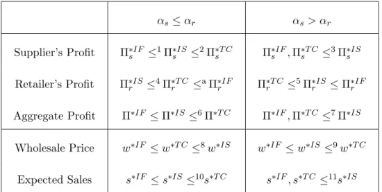
Table 1.1 summarizes our comparison results. Π∗, Π∗rand Π∗sdenote the expected aggregate profits and that of the supplier and the retailer, respectively, whilew∗ and
s∗ denote the equilibrium wholesale price and the expected sales volume per period. Superscripts indicate which of the three financing mechanisms the measure refers to. All inequalities with a numbered footnote are proven in the paper, the footnote indicating where precisely. The remaining rankings are based on the above extensive numerical study reported.
The above structural results for the Stackelberg games carry over to to the two generalized models considered in this paper, where the retailermay default. In this case some or all of the creditors receive only part of the amount due to them, the so-called recovery rate. In the first generalized model, we assume only the supplier faces this default risk when engaging in a TC arrangement while the bank has immunized itself from this risk; in the second generalization, both the supplier and the bank face default risks. As to the comparison results across these financing mechanisms, they carry over to the first generalized model in the sense that many rankings can be established by comparingαr with an index that depends onαs, the recovery rate
αs ≤αr αs> αr Supplier’s Profit Π∗sIF ≤1Π∗IS s ≤2Π∗sT C Π∗sIF,Π∗sT C ≤3Π∗sIS Retailer’s Profit Π∗rIS ≤4Π∗T C r ≤aΠ∗rIF Π∗rT C ≤5Π∗rIS ≤Π∗rIF Aggregate Profit Π∗IF ≤Π∗IS ≤6Π∗T C Π∗IF,Π∗T C ≤7Π∗IS Wholesale Price w∗IF ≤w∗T C ≤8w∗IS w∗IF ≤w∗IS ≤9w∗T C Expected Sales s∗IF ≤s∗IS ≤10s∗T C s∗IF, s∗T C ≤11s∗IS
Table 1.1: Comparisons among the financing schemes 1-2: See Proposition 2.4 (i) and Theorem 2.5 (b) for a proof, respectively.
3: See Proposition 2.4 (i) and Theorem 2.5 (b) for a proof. 4-5: See Theorem 2.6 (c) for a proof.
6: It follows from inequalities in footnotes 2 and 4
7: Π∗T C≤Π∗IS follows from inequalities in footnotes 3 and 5.
a: It holds numerically in all but nine instances. The nine exceptions are instances where the supplier’s cost of capital is substantially lower than that of the retailer and the variable profit margin (p−c)/c= 0.11 is small. The small profit margin severely limits the supplier’s ability to raise the price while his significant capital cost rate advantage allows for major profit improvement compared to IF.
8-9: See Theorem 2.6 (e) for a proof. 10-11: s∗T C ≤s∗IS follows from Theorem 2.6 (d).
model with default risks, these comparisons need to be made numerically.
1.3
Inventory Models with Shelf Age and Delay
Depen-dent Inventory Costs
One of the main objectives of any inventory planning model is to analyze the trade-off between competing risks of overage and underage. This requires an adequate representation of the carrying costs associated with all inventories, as well as the cost and revenue consequences of shortages. Early contributors, e.g., the pioneer-ing textbooks by Hadley and Whitin (1963) and Naddor (1966), discussed possible paradigms to represent the carrying and shortage costs.
One standard paradigm is to assume that carrying costs can be assessed, either continuously or periodically, as a (possibly non-linear) function of the prevailing total inventory, irrespective of its age composition. Similarly, shortage costs are assumed to accrue as a(, again, possibly non-linear) function of the total shortfall or backlog, irrespective of the amount of time the backlogged demand units have remained unfilled. We refer to this type of carrying and shortage cost structures as level-dependent inventory costs. After the above mentioned early discussions in Hadley and Whitin (1963) and Naddor (1966), this paradigm has been adopted in virtually every inventory model.
There are, however, many settings where carrying costs need to be differenti-ated on the basis of the inventory’s shelf-age composition. First, inventories are often financed by trade credit arrangements, where the supplier allows for a pay-ment deferral of delivered orders, but charges progressively larger interest rates as the payment delay increases. For example, the supplier frequently offers an initial interest-free period (e.g., 30 days) after which interest accumulates. Moreover, in-terest rates often increase as a function of the item’s shelf age. These trade credit schemes have been considered in Gupta and Wang (2009) as well as Chapter 2. We refer to the latter for a discussion of how prevalent this practice is. Another setting with shelf age dependent inventory cost rates arises when the supplier subsidizes
part of the inventory cost. For example, in the automobile industry, manufactur-ers pay the dealer so-called “holdbacks”, i.e., a given amount for each month a car remains in the dealer’s inventory, up to a given time limit (see, e.g., Nagarajan and Rajagopalan (2008)). The resulting inventory cost rate for any stocked item is, again, an increasing function of the item’s shelf age.
Even when inventory costs grow as a linear function of the loan term or the amount of time the purchased units stay in inventory,time varying purchase prices or interest rates necessitate disaggregating inventory levels according to the time at which the units were purchased, i.e., in accordance with the items’ shelf age. As an example, in the dynamic lot sizing literature, Federgruen and Lee (1990) modeled holding costs as proportional to the items’ purchasing price, which varies with their purchase period. As a consequence, holding costs depend on the items’ shelf age. Even more general shelf-age dependencies are assumed in Levi et al. (2011) and its generalization, i.e., so-called metric holding costs, in Stauffer et al. (2011). Finally, beyond capital costs, inventories often incur maintenance related expenses; these, too, vary as a function of the items’ shelf age.
Similar to shelf age dependent holding costs, backlogging costs may also depend on the amount of time by which delivery of a demand unit is delayed. This may reflect the structure of contractually agreed upon penalties for late delivery or, in case of implicit backlogging costs, the fact that customers become less or more impatient over time. This type of backlogging costs has been studied by Chen and Zheng (1993), Rosling (1999, 2002) and Huh et al. (2010).
In this paper, we show how periodic and continuous review models with a general
shelf age dependent holding cost structure may be transformed into an equivalent “standard” model in which all expected inventory costs are level-dependent. These equivalency results allow for the rapid identification of the structure of an optimal policy, in various models. It also allows for the immediate adoption of algorithms to compute optimal policies. Moreover, in periodic review models, all shelf age dependent inventory holding cost components are transformed into linear holding costs, however, with a specific modified random leadtime distribution.
We develop our equivalency result, first, for models with full backlogging of stockouts. These models allow for a one-dimensional state representation via the so-called inventory position, i.e., on-hand inventory + outstanding orders - back-logs. This equivalency result permits us to characterize the optimal procurement strategy in various settings. For example, assuming demands are independent with exogenously given distributions, a simple time-dependent (s, S) policy, acting on the inventory position is optimal under fixed-plus-linear order costs. In the absence of fixed delivery costs, this structure further simplifies to that of a base-stock policy. In the special case where all model parameters are stationary, we show that the base-stock levels increase as we progress to the end of the planning horizon; moreover these levels can be determined myopically by computing, for each period, the min-imum of a period specific, closed-form convex function. When each of the demand distributions depends on the buyer’s retail price, the optimal combined inventory and pricing strategy is a so-called base-stock/list price policy, assuming no fixed ordering costs prevail, and leadtimes are negligible. In the presence of such fixed costs, and assuming the stochastic demand functions have additive noise terms, the optimal combined strategy is of the so-called (s, S, p) structure: the procurement part of the combined strategy continues to be of the (s, S) type. Other variants of this model and of the associated optimal strategies are discussed as well.
We generalize our equivalency results for models in which all or part of stockouts are lost. Here, the state of the system needs to be described with a multi-dimensional inventory vector: more specifically, under a positive leadtimeL >0, it is well known that the state of the system needs to be represented by an (L+ 1)- state vector, keeping track of the inventory on hand and all outstanding orders from the last L
periods, separately. Here, we show that the addition of any shelf age dependent cost structure does not complicate the structure of the model beyond what is required under the simplest, i.e., linear holding costs.
A different transformation, due to Huh et al. (2010), allows for the treatment of general delay dependent backlogging cost structures, but only under an assumption guaranteeing either that no demand unit is delayed by more than the leadtime plus
one periods, or that the incremental backlogging cost rate is constant for delays in excess thereof. The first condition is equivalent to assuming that the inventory position after ordering is always non-negative. We review this transformation in §3.1.3, and prove various optimality results that can be obtained under general delay dependent cost structures.
In §3.2, we show how general shelf age dependent holding and delay dependent backlogging costs can be handled in continuous review models. Starting with the case of renewal demand processes, we show that, for these, an equivalent model with a convex, inventory level dependent cost structure can be obtained, in full generality, i.e., without any policy restrictions. This equivalency result is based on a very different so-called “single unit decomposition approach”, in the spirit of those introduced by Axs¨ater(1990, 1993) and Muharremoglu and Tsitsiklis (2008). The equivalency result allows us to conclude, for example, that in a system with fixed-plus-linear ordering costs, an (r, q)- policy is optimal, and the long run average cost as a function of r and q, is of a structure enabling the use of the algorithm in Federgruen and Zheng (1992) to identify the optimal parameters. Finally we char-acterize how various model primitives such as the leadtime distribution, the shape of the marginal shelf age dependent cost function and that of the delay dependent backlogging cost function impact the optimal policy parametersr∗andR∗ ≡r∗+q∗. We also show (in §3.2.2) that the results for periodic inventory systems carry over to continuous review models with generalcompound renewal demand processes. We show that under minor assumptions, the model is equivalent to a periodic review model with convex inventory level dependent carrying and backlogging costs. Under fixed-plus-linear costs, this implies, for example, that an (s, S) policy is optimal.
1.4
Monotonicity Properties of Stochastic Inventory
Sys-tems
In the past fifty years, a voluminous literature has arisen on inventory models. In many elementary models, we are able to prove that the optimal procurement
strategy has a relatively simple structure characterized by a few policy parameters. Moreover, for several of those models, we have identified efficient algorithms, able to compute the optimal combination of policy parameters.
Nevertheless, most of these models fail to be used widely by practitioners or to be taught in Operations Management classes or textbooks, with the exception of Economic Order Quantity (EOQ)- and newsvendor type models. The continued popularity of the latter two classes of inventory models can not be attributed to the applicability of the underlying model assumptions, which, in fact, are very restrictive and fail to fit many of the settings where they are routinely applied. Instead, their continued popularity is based on the fact that they allow for closed form expressions of the optimal policy parameters, thus providing easy and immediate insights into how various model primitives (cost parameters, demand processes, leadtimes etc.) impact on the above policy parameters. As articulated by Geoffrion (1976), the main purpose of models is to provide “insights, not numbers”. At the most basic level, the model user wishes to understand whether optimal policy parameters and associated performance measures increase or decrease as a function of the various model primitives.
In this paper, we derive general conditions under which monotonicity of the optimal parameters and associated key performance measures, with respect to gen-eral model primitives, can be established within a (single-item) inventory system governed by an optimal (r, q) or (r, nq) policy. Under an (r, q) policy, the system is monitored continuously and a replenishment order of a fixed size q is placed whenever the inventory position drops to the levelr. When the demand process ex-periences jumps of an arbitrary magnitude, it is sensible to apply an (r, nq) policy, with the order quantity specified as the minimum multiple of q required to bring the inventory position back above the reorder level r. (r, q) or (r, nq) policies are also frequently used in serial systems, see, e.g., Shang and Zhou (2009, 2010). In contrast to the above EOQ related deterministic models, the optimal (r, q) or (r, nq) policy parameters can not be obtained in closed-form, but need to be computed al-gorithmically, even under the simplest demand processes, i.e., Brownian motions or
Poisson processes. Prior literature, reviewed in the next section, has studied the impact of changes of a fewspecific model primitives, in particular, the leadtime and the leadtime distributions.
Many key performance measures are directly related to the optimal policy pa-rametersr∗,R∗ ≡r∗+q∗ andq∗. Operations managers are concerned with the max-imum inventory (position), the average inventory level and the minmax-imum inventory, the latter being related to the so-called safety stock concept. Logistics managers focus on the average order size or order frequency, its reciprocal. Suppliers often prefer a regular order pattern associated with high order frequency to allow for a smooth production/distribution schedule. Financial analysts and macroeconomists pay particular attention to the sales/inventory ratio, also referred to as the inventory turnover.
Beyond providing general insights into inventory systems governed by (r, q) or (r, nq) policies, the above monotonicity properties have additional benefits: first, many of the parameters or distributions in the model are difficult to forecast and the model user needs to understand in which direction an under- (or over-)estimate biases the optimal policy parameters. Second, the monotonicity properties can be exploited when the model needs to be solved repeatedly for many parameter val-ues. This situation arises either because of uncertainty about a parameter or be-cause service level constraints are added to the model which, when handled via Lagrangian relaxation, requires the repeated optimization of a traditional aggregate cost function for many multiplier values or combinations thereof. (Such service level constraints include constraints on thefill rate, i.e., the fraction of demand that can be filled immediately without backlogging, or the ready rate, i.e., the fraction of time the system has stock, or the expected amount of time a backlogged demand has to wait before being filled.) If it is known that an increase in a parameter or Lagrange multiplier from a valueµ0 toµ1 results in an increase or (decrease) ofq∗, say, this fact can be exploited, for example, when using the algorithm in Federgruen and Zheng (1992): when re-optimizing the model for µ= µ1, one may, then, start
Appendix.
Depending upon whether the sample paths of the leadtime demand process are continuous or step functions, the long-run average cost is of the form:
c(r, q|θ) = λK+ Rr+q r G(y|θ)dy q , (1.1) or c(r, q|θ) = λK + Pr+q y=r+1G(y|θ) q . (1.2)
In both (1.1) and (1.2), λand K represent the long-run average demand rate and the fixed cost incurred for every order batch of size q respectively. All other model primitives θ ∈ Θ impact the long-run average cost exclusively via the so-called instantaneous expected cost functionG(y|θ). When the long-run average cost of an (r, q) or (r, nq) policy is given by (1.1)[(1.2)], we refer to the model as the continuous [discrete] model. Since the representations in (1.1) and (1.2) are common under (r, q) or (r, nq) policies, we henceforth confine ourselves to the former, without loss of generality.
The fixed costKimpacts only the first term in the numerator of (1.1) and (1.2). Zheng (1992) already showed that the optimal reorder levelr∗is decreasing while the optimal order size q∗ and the optimal order-up-to level R∗ ≡r∗+q∗ are increasing in this parameter1. In contrast, the average demand rateλimpacts both terms in the numerator of the long-run average cost function and the net monotonicity effect on the optimal policy parameters is therefore, sometimes, ambiguous2. We establish our monotonicity properties with respect to all other general model primitivesθ∈Θ, merely requiring that the space Θ be endowed with a partial order . As such, θ
may be a cost parameter, or a parameter of the demand or leadtime distribution. Alternatively, θ may represent the distribution of a random variable or a complete stochastic process, or a cost rate function.
1
Zheng (1992) confines himself to the continuous model; A similar treatment of the discrete model can easily be obtained based on the algorithm in Federgruen and Zheng (1992).
2
Our first main result is that the optimal reorder levelr∗ and the optimal order-up-to level R∗ are decreasing (increasing) in θ whenever the functionG(y|θ) is su-permodular (submodular) in (y, θ), that is, any of the difference functionsG(y2|θ)−
G(y1|θ), withy1 < y2, is increasing (decreasing) in θ. Thus, the monotonicity
pat-terns ofr∗ andR∗ are identical in the continuous model (1.1) and the discrete model (1.2) and the general conditions under which they are obtained are identical as well. As to the remaining policy parameter q∗, i.e., the optimal order quantity, here the monotonicity patterns that can be expected, differ themselves, between the con-tinuous model (1.1) and the discrete model (1.2). In the concon-tinuous model, we show that q∗ can often be guaranteed to be monotone in various model parame-ters. In the discrete model, occasional unit increases (decreases) between stretches whereq∗(θ) is decreasing (increasing) can not be excluded. This gives rise to a new monotonicity property which we refer to as rough monotonicity: an integer valued function is roughly decreasing (increasing) if the step function does not exhibit any pair of consecutive increases (decreases). We show that pure monotonicity of q∗ in the continuous model andrough monotonicity in the discrete model, with respect to any model parameter, can be guaranteed if the supermodularity or submodularity property ofG(·|θ) function is combined with a single additional structural property of this instantaneous expected cost function. While the conditions in the continous and discrete model are very similar, the required analysis is fundamentally different. Finally, we identify a broad sufficient condition for monotonicity of the optimal cost value; to our knowledge, this condition encompasses all known applications as well as several new ones.
The most frequently used model in which the long-run average cost of an (r, q) or (r, nq) policy is given by (1.1) or (1.2), has the following assumptions: the item is obtained at a given price per unit; inventory costs are accrued at a rate which is a convex increasing function of the inventory level; stockouts are backlogged where backlogging costs are, again, accrued at a rate which is a convex increasing function of the backlog size; leadtimes are generated by a so-called exogenous and sequential process, ensuring that consecutive orders do not cross and the leadtimes
are independent of the demand process. We refer to this as the standard inventory model.
For these standard inventory models, our general results imply, in particular, that r∗ and R∗ are decreasing in the item’s purchase price, assuming that the in-ventory carrying cost rate function increases monotonically with the purchase price. Similarly, r∗ and R∗ are decreasing in other parameters on which the marginal in-ventory carrying cost rate function depends monotonically, for example, the physical maintenance and warehousing cost per unit of inventory, or more generally, when the marginal holding cost rate function is replaced by a pointwise larger one. In contrast, r∗ and R∗ are both increasing when the marginal backlogging cost rate function is replaced by a pointwise larger one. As a final application for the standard inventory model, compare two leadtime demand processes such that the leadtime demand distribution under the first process is stochastically smaller than that under the second process. (Dominance of the steady-state leadtime demand distribution may arise because of a change of the demand process, a stochastic enlargement of the leadtime distribution, or both.) We show that r∗ and R∗ are always smaller under the first process compared to the latter. As far as q∗ is concerned, our gen-eral results imply, for example, monotonicity with respect to the purchase price and holding cost rates, assuming that the leadtime demand distribution is log-concave or log-convex, a property shared by most classes of distributions. Similarly, q∗ is monotone in the backlog cost rate if the complementary cumulative distribution of the leadtime demand distribution is log-cave or log-convex. In the case of normal leadtime demands,q∗ is monotone in their mean and standard deviation. Similarly, if the demand process is a Brownian motion and leadtimes are fixed,q∗is increasing in the drift and volatility of the Brownian motion and in the leadtime. Sufficient con-ditions for (rough) monotonicity can often be stated in terms of broadly applicable properties of the cdf of the leadtime demand distribution such as log-concavity.
Chapter 2
Inventory Subsidy versus
Supplier Trade Credit in
Decentralized Supply Chains
We refer to Section 1.2 for an introduction of this chapter. In Section 1.2 we intro-duced the following three fundamental financing options:
(I)Independent Financing(IF): this reflects the traditional business model where the retailer finances her inventories through a bank or by drawing from her own cash reserves, without any supplier involvement.
(II) Inventory Subsidies (IS): same, except that the supplier offers to cover a specific part of the capital costs associated with the retailer’s inventories.
(III) Trade Credit (TC): here the supplier adopts the financing role otherwise assumed by a bank or the retailer herself, as in (I) and (II).
This chapter is organized as follows. §2.1 reviews related literature. In§2.2 we model the supply chain under the IF, IS and TC financing schemes. We show that all three models can be synthesized into a single unified model. For this unified model, §2.3 characterizes the equilibrium behavior of the first Stackelberg game with an exogenously given inventory subsidy or trade credit interest charge. §2.4 achieves the same for the remaining two Stackelberg games, i.e., the game with an
exogenously given wholesale price and the full Stackelberg game, and is followed by a brief§2.5 in which the various structural results for the three games are summarized. §2.6 derives the above mentioned comparison results among the three financing mechanisms. In§2.7 we develop the two generalized models with default risks. The final§2.8 summarizes our findings and discusses other variants of our models.
2.1
Literature Review
Several papers in the operations management literature have analyzed the interac-tion between suppliers and retailers facing demand risks, under one of the above mentioned payment schemes. Most of the literature confines itself to a single sup-plier servicing a single retailer. The specific payment terms are either assumed to be selected by the supplier so as to maximize his profits, or by a third party (coor-dinator) so as to maximize chain wide profits. The former perspective gives rise to a Stackelberg game with the supplier as the leader, while in the latter the central question is whether a perfect coordination mechanism exists and if so how these parameters are to be selected.
Wholesale price only contract
The first Stackelberg game model in this general area is Lariviere and Porteus (2001), considering a single period model under a simple constant wholesale price scheme without any additional incentives, as in IF. The authors show that the sup-plier’s equilibrium profit function under the retailer’s best response is unimodal in the wholesale price as long as the demand distribution satisfies a generalization of the IFR property, which the authors refer to as IGFR (Increasing General Fail-ure Rate). See Lariviere (1999) and Cachon (2003) for detailed reviews of this model. Numerical studies in these papers show that the chain wide profits under the Stackelberg solution are 20-30% below those obtained in the centralized solu-tion. However, perfect coordination can only be achieved when the wholesale price equals the supplier’s variable cost rate as shown by Pasternack (1985), resulting in an unsatisfactory arrangement where the supplier’s profits are reduced to zero.
Wholesale price and inventory subsidy contract
Anupindi and Bassok (1999) and Cachon and Zipkin (1999) appear to be the first to consider the inventory cost subsidy as a mechanism by the supplier to as-sume part of inventory risks. As in IS, the former asas-sume that the retailer(s) obtain independent financing for their purchases, while the supplier assumes part of the resulting financing/inventory costs. Considering a periodic review infinite horizon model, Anupindi and Bassok (1999) deals, among others, with settings where all retail demand is satisfied from a single stocking point. The authors analyze both the Stackelberg game that arises when the wholesale price is given and the supplier selects his subsidy of the inventory cost rate as well as the Stackelberg game that prevails when the wholesale price is chosend, but only in the special case of inven-tory cost subsidies. For the latter Stackelberg game, Anupindi and Bassok (1999) show that under Normal demands, an approximation for the equilibrium supplier’s profit function is concave. For the former game, unimodality is verified numerically. We prove that the exact supplier’s equilibrium profit function is unimodal in both Stackelberg games for a broad class of demand distributions which include the Nor-mals as a special case, and for arbitrary choices of the exogenously specified contract terms. In addition, we characterize the (full) Stackelberg game which arises when the supplier controls both his wholesale price and his inventory subsidy. The single period model in Zhou and Groenevelt (2008) may be viewed as a variant of the Stackelberg game under a given inventory subsidy, indeed, the extreme case where the supplier assumes all the inventory costs. These authors also incorporate the possibility of a retailer going bankrupt when his loss exceeds a certain threshold. Another departure from the literature is the assumption that the retailer’s capital cost rate isendogenously selected by the bank along with a maximum percentage of the purchase order which he is willing to finance. The bank selects these financing terms in advance of the supplier’s wholesale price so as to break even in expectation. Other papers have established that inventory subsidies may be used as an essen-tial component of coordination mechanisms, again in a supply chain with a single supplier and a single retailer. Cachon and Zipkin (1999) establish this in an infinite
horizon model, assuming both chain members employ a base-stock policy. Similarly, Wang and Gerchak (2001) show, in a single sales period model, that a combined wholesale price/inventory cost rate subsidy contract achieves perfect coordination in the supply chain. (The demand distribution may depend on the stocking level.) The availability of an inventory cost rate subsidy as a lever allows for a continuum of coordination mechanisms beyond the single and unsatisfactory (wholesale price only) mechanism identified by Pasternack (1985). Narayanan et al. (2005) analyze the same combined wholesale price/inventory cost rate subsidy contracts to coor-dinate a supply chain consisting a supplier and two retailers. Finally, Nagarajan and Rajagopalan (2008) consider inventory subsidies in the context of Vendor Man-aged Inventories where an inventory cost rate subsidy is specified as part of the contractual agreement.
Wholesale price and trade credit contract
Kouvelis and Zhao (2009) and Yang and Birge (2011) have analyzed settings where the supplier himself acts as the financing institution, offering a trade credit option. In the former’s Stackelberg game model, the supplier specifies a cash-on-delivery wholesale price and a capital cost rate for units paid at the end of the sales period. As in Zhou and Groenevelt (2008), the authors assume that the retailer’s ability to pay upfront is constrained by her initial cash balance and they incorporate the possibility of bankruptcy at the end of period. This supplier financing scheme is compared with the one in which an outside bank finances the units bought on credit. As in Zhou and Groenevelt (2008), the interest rate is determined so that the bank breaks even in expectation. Yang and Birge (2011) consider a variant of this model, incorporating credit limitations for the supplier and a liquidation or distress cost in the event of bankruptcy.
Other related papers include Gupta and Wang (2009) who characterize the re-tailer’s optimal procurement strategy under a TC payment scheme. In their paper, the supplier charges interest as a general nonlinear function of the amount of time elapsed between the delivery of goods and the payment. The authors show that under the standard linear holding and backlog cost the base-stock policy is optimal.
In Chapter 3, we provide a simple proof and extend the structural result for the optimal procurement policy to many other settings, for example, those with fixed procurement costs and/or price-dependent demand.
Finally, we refer to Buzacott and Zhang (2004) and references there for a limited stream of papers addressing the important topic of inventory management under credit restrictions in a single firm setting.
2.2
Model
We characterize the interaction between the supplier and the retailer in an infinite horizon periodic review system. We choose an infinite planning horizon so as to model an ongoing trade relationship between the supplier and the retailer involving many repeated procurement decisions for storable items. (The stationary infinite horizon model is a standard framework in the supply chain literature when repre-senting repeating procurement decisions, see for example Cachon (2003) and Zipkin (2000).) While some inventory models involve parameters and distributions that fluctuate cyclically or, in dependence of a more general exogenous state variable, the treatment of such phenomena appears tangential to the questions raised in this paper and complicates its analysis and results needlessly. In other words, there is no reason to believe that the schemes’ relative advantages and disadvantages differ in environments with stationary versus fluctuating parameters. See, however, §2.8 for a generalization of our model in which interest rates fluctuate stochastically.
The retailer faces a sequence of independent and identically distributed customer demands under an exogenously given retail price. She may place a purchase order with the supplier at the beginning of any period. Orders placed at the beginning of a period arrive in time to satisfy that period’s demand. Unsatisfied demand results in lost sales. As a consequence, the retailer’s sales volume, and hence, that of the sup-plier depend on the retailer’s inventory replenishment strategy; the latter, in turn, depends on the structure of the selected supplier financing scheme. We distinguish between two types of inventory carrying costs: (i) physical storage and maintenance
costs, assumed to be proportional with each end-of-the-period inventory level, (ii) financing costs, the structure of which depends on the specific terms of the payment scheme in place. In the base model, we assume that the likelihood of the retailer defaulting on her payment is negligible. See, however, §2.7 for generalizations that allow for defaults.
Let D = the random demand observed in an arbitrary period, with a known cdfF(y), continuously differentiable pdf f(y), mean µ <∞ and standard deviation
σ <∞.
p= the per unit retail price.
c= the per unit supplier’s variable procurement cost rate.
h0 = the physical (storage and maintenance) cost per unit carried in inventory
at the end of a period.
As mentioned in the Introduction, αr denotes the capital cost rate incurred by the retailer under independent financing, that is when drawing from her own cash reserves or from a credit line offered by the bank. (The size of the cash reserves or the credit line is assumed to be ample.) In the former (latter) case, αr represents
the rate of return on its best alternative investment option (bank loan rate). If both capital sources are available, αr denotes the lower of the two rates. αs denotes the
capital cost rate incurred by the supplier, determined analogously.
Even ifαr andαs both represent bank loan rates, significant differences between
these rates arise because of variety of factors. These include the firm’s country or region, the industry it belongs to, the size of the credit line, the size of the firm (measured by its assets or gross revenues), the loan type, as well as its overall financial credit record and several financial ratios on its balance sheet and profit/loss statement1. Several papers have estimated the relative importance of these factors
1
Bank rates for commercial loans and credit lines are determined as a spread with respect to a base rate, for example LIBOR (The London Interbank Offered Rate) or the U.S. prime rate. Firms are assigned one of a small number of possible risk ratings based on public or private bond ratings, the above mentioned financial ratios and its liquidity of the collateral provided (see, for instance, Koch (1995)). The dependency of bank rates on these characteristics is apparent in publicly available databases such as DealScan.
from large databases of bank loans, e.g., Berger and Udell (1990, 1995), Booth (1992), Petersen and Rajan (1994), Beim (1996) and Fernandez et al. (2008). While identifying many factors that explain major differences in bank loan rates, these studies conclude that the role of the borrower’s default risk is either insignificant or only of moderate importance2.
In addition, all the above loan rate determinants represent characteristics of the firm’s past and global performance across all of its business units and product lines, as opposed to the specific product line considered here. Since in this paper we focus on firms with many markets and product lines, we treat, both under self-and bank-financing, the capital cost rates αs and αr as exogenous parameters (or
exogenous stochastic processes, see§2.8), analogous to their treatment in almost all of the inventory and supply chain literature.
2.2.1 Independent Financing (IF)
Under IF, the retailer finances her inventories with a bank, or from her own cash reserves (self-financing), i.e., the supplier is paid immediately upon delivery of the procurement orders either by the bank or through self-financing. In the former case, IF is often implemented through factoring where the purchase invoice is owed to the bank, and the retailer draws from a credit line; in the latter case the purchasing invoice is paid from and owed to the firm’s cash reserves. The supplier charges a constant wholesale pricew. It is optimal for the retailer to determine its procurement decisions in accordance with a base-stock policy, say with base-stock levely. (Under a base-stock policy, the inventory level is increased to the base-stock level in any period whose starting inventory is below that level.) Let
s(y) =Emin{D, y}= the expected retailer sales per period under a base-stock
policy with base-stock level y,
2Beim(1996), for example, states “Factors which are important in bond pricing, such as borrower
risk and loan term, have only moderate importance in bank lending, while other factors such as borrower size and geographic location, lender identity, and pricing benchmark have unexpectedly high significance.”
h(y) = E(y −D)+ = the expected end-of-the-period inventory level under a
base-stock policy with base-stock levely.
h(y) also denotes the expected number of units at the end of a period that have been received by the retailer but not yet paid for under the base-stock policy, so that
wh(y) represents the average per period amount of outstanding debt to the bank or the firm’s own cash reserves, which is charged at a capital cost rate αr, either by
the bank or by drawing from the retailer’s own cash reserves.
The profit functions of the retailer and the supplier are therefore given by:
πIFr (w, β, y) = (p−w)s(y)−(αrw+h0)h(y), πsIF(w, β, y) = (w−c)s(y)
2.2.2 Inventory Subsidies (IS)
Under IS, the retailer continues to finance her inventories with a bank, or from her own cash reserves. However, the supplier offers to subsidize the retailer’s holding cost, specifically the capital cost component. Let β be the subsidy rate where 0≤β ≤αr. Thus the effective capital cost rate of the retailer is αr−β. The profit
functions of the retailer and the supplier are now given by:
πrIS(w, β, y) = (p−w)s(y)−[(αr−β)w+h0]h(y), πISs (w, β, y) = (w−c)s(y)−βwh(y).
Note that IF is a special case of IS withβ = 0. 2.2.3 Trade Credit (TC)
Under TC the supplier adopts the financing function, permitting the retailer to delay payments for purchased goods until the time of sale3. The supplier charges the retailer a given interest rate for each period during which payment for an item is outstanding. This per period interest rate may vary as a function of the item’s shelf age4.
3In practice, the due date is often selected as a fixed calendar day, decoupled from the time of
sale. 4
For example, the supplier may charge a flat rate from the time of delivery, or he may offer an initial grace period of Gperiods without any interest charges, followed by a constant interest
To provide a fair comparison of IF and IS, we confine ourselves to the case where the supplier charges a flat interest rateα ≤αr irrespective of the item’s shelf age.
At the same time, we consider both the case where α ≥ αs and the one where
α < αs, i.e., the supplier either incurs a net revenue or a net cost when extending
trade credit to the retailer. As under IF and IS, it is easily verified that a base-stock policy continues to be optimal for the retailer5. Usingy to denote the base-stock level, the expected amount of payables at the end of each period equals wh(y), as before. This results in an expected per period cost αwh(y) to the retailer, and an equivalent revenue for the supplier. The supplier finances his working capital at a cost rateαs, either by his bank or drawing from his cash reserves, therefore the net
interest revenues for the supplier are given by (α−αs)wh(y). We conclude that the chain members’ profit functions are now given by:
πrT C(w, α, y) = (p−w)s(y)−(αw+h0)h(y), πT Cs (w, α, y) = (w−c)s(y)+(α−αs)wh(y).
2.2.4 A General Model
The IF, IS and TC models are special cases of the following general model.
πr(w, βg, y) = (p−w)s(y)−[(α−βg)w+h0]h(y) (2.1)
πs(w, βg, y) = (w−c)s(y)−βgwh(y) (2.2) Hereβg represents the supplier’s effective capital cost rate (ECCR), a term of trade to be selected by him along with the wholesale price w. Moreover, the supplier’s ECCR βg is to be selected in a given interval [α, α] with α ≤α. Note thatα−βg
may be interpreted as the retailer’s ECCR.
rateα1, applied to any additional period. As a third example, the interest rate may be increased to a levelα2 > α1 for units purchased more than G2 periods ago. In general, as in Gupta and Wang (2009), let α(t) be the incremental interest rate charged for any unit with a shelf age oft
periods, i.e., whose payment has been outstanding fortperiods, and assume thatα(·) is an arbitrary non-decreasing function.
5This structural result continues to apply under general increasing shelf-age dependent interest
rate function α(·), see Gupta and Wang (2009) and Chapter 3. Chapter 3 also characterize the optimal procurement policy under more general cost and revenue structures.
We obtain the IS model by setting βg =β,α = 0 and α =αr. The IF model has the same parameters as IS except thatβg= 0. The TC model can be obtained
by selectingβg =αs−α,α=αs−αr and α=αs.
It is well known and easily verified that in the general model, the retailer’s optimal base-stock level y(w, βg) in response to given trade terms (w, βg) is given by a specific fractile of the demand distribution. More specifically, y(w, βg) is the
fractile that satisfies
F(y) = 1− (α−βg)w+h0
p−w+ (α−βg)w+h0
. (2.3)
Note thaty(w, βg) is decreasing inw and increasing inβg.
Next in §2.3-2.4, we focus on the general model specified by the profit functions (2.1) and (2.2) and characterize the equilibrium behavior in three distinct Stackel-berg games with the supplier as the leader and the retailer as the follower. In the first Stackelberg game the supplier selects the wholesale price under an exogenously given ECCR βg; In the second Stackelberg game the supplier selects his ECCR
un-der a given wholesale price w, while in the third game the supplier controls both terms of trade, wand βg.
2.3
The Stackelberg Game under a Given ECCR
Given the supplier’s ECCRβg, he chooses his optimal wholesale price on the interval [0, p], taking into account the retailer’s best response procurement strategy. (In some settings, the supplier may offer the product at a wholesale price below the variable cost rate while still realizing a profit on the basis of the finance charges.) This gives rise to the equilibrium profit function ˆΠs(w|βg) ≡ πs(w, βg, y(w, βg)).
Analysis of the Stackelberg game requires an understanding of the structure of the equilibrium profit function ˆΠs(·|βg). However, it is more convenient to express the
supplier’s equilibrium profit as a function of the retailer’s base-stock level y, as opposed to his wholesale price. Since the retailer’s optimal base-stock levely(w, βg) is strictly decreasing in w, we can write w as a function of y. Let w(y) denote the
inverse function, i.e.,
w(y)≡ p−(p+h0)F(y)
1−(1−δ)F(y) , (2.4)
where δ =α−βg ≥0.The supplier’s equilibrium profit, as a function of the base-stock level y, is thus given by: Πs(y|βg) = (w(y) −c)s(y)−βgw(y)h(y). After
determining the optimal targeted base stock level y∗βg, the corresponding wholesale price that induces this base stock level is immediate from (2.4).
The supplier’s equilibrium profit as a function of y can be written as
Πs(y|βg) =w(y)(s(y)−βgh(y))−cs(y) =w(y)ξ(y)−cs(y). (2.5)
whereξ(y)≡s(y)−βgh(y). In other words, if the supplier assumes part of the capital
costs associated with the retailer’s inventory, either in a TC or IS arrangement, this is equivalent to accepting a reduction of the expected sales volume per period s(y) to the lower quantity ξ(y), where the correction term is strictly proportional to the ECCRβg. We therefore refer toξ(y) as the supplier’seffective expected sales volume,
in contrast to thegross expected sales quantitys(y). In terms of the gross expected sales quantity, it is always in the supplier’s interest to induce a higher base-stock level. Since ξ0(y) = 1−(1 +βg)F(y), the effective expected sales volume increases with the base-stock level but only up to the 1/(1 +βg)-th fractile of the demand
distribution, i.e., ξ0(y) = 1−(1 +βg)F(y)>0 if and only if y < ys≡F−1 1 1 +βg . (2.6) (In case βg = 0, define ys ≡ ∞.) Clearly, the supplier has no interest in targeting a base-stock level above this critical fractile ys: for any y > ys, either the effective
expected sales volume itself is negative, resulting in negative profits, or the marginal profit Π0(y|βg) < 0 since w0(y) < 0, ξ0(y) < 0 and s0(y) > 0. In other words, the
critical fractile ys is a natural bound for the targeted base-stock level.
Similarly, a second natural bound for the targeted base-stock level is given by the 1/(1 +h0/p)-fractile, that isF−1(1/(1 +h0/p)). To verify this, note from (2.3)
thatF(y) is a decreasing function ofw, so thatF(y) is bounded from above by the expression for the right-hand side of (2.3), obtained when w = 0. Combining the
two upper bounds, we specify, without loss of generality, that ymax≡min ys, F−1 1 1 +h0/p =F−1 1 1 + max{h0/p, βg} . (2.7)
(As above, in case βg = h0 = 0, define ymax ≡ ∞.) We now show the supplier’s
equilibrium profit is quasi-concave is quasi-concave both as a function of the base-stock level and as a function of the wholesale price.
Theorem 2.1(Stackelberg game under given ECCR) Assume the demand distribu-tion is IFR. (a) The supplier’s equilibrium profitΠs(·|βg)is quasi-concave on the full base-stock level range [ymin = 0, ymax], achieving its maximum at a unique interior pointyβ∗
g.
(b) The supplier’s equilibrium profitΠˆs(·|βg), viewed as a function ofw, is quasi-concave on the wholesale price range [0, p], achieving its maximum at a unique in-terior pointwβ∗
g =w(y ∗
βg), and with limw↑p ˆ
Πs(w|βg) = 0.
Anupindi and Bassok (1999) address this Stackelberg game in the special case of IF arrangements withh0 = 0. The authors state that they are unable to determine
if the supplier’s equilibrium profit function is “convex, concave, or even unimodal in the wholesale price”. This contrasts Lariviere and Porteus (2001), dealing with thesingle period Stackelberg game under IF, who show that the supplier’s equilib-rium profit function is quasi-concave under a generalization of the IFR condition. (Indeed, the structure of the profit functions in a single period model is essentially simpler.) Anupindi and Bassok (1999) obtain a characterization of the structure of the supplier’s equilibrium profit function only for Normal demand distributions and under Nahmias (1993)’ approximation of the inverse of the standard Normal cdf by a difference of power functions. Returning to single period models, Kouvelis and Zhao (2009) address a variant of the Lariviere and Porteus (2001) model with a bank loan rate endogenously determined so that the bank breaks even in expecta-tion, considering the possibility of default. The authors show that in this case the Stackelberg game reduces to that of Lariviere and Porteus (2001) with the capital cost rate given by the bank’s cost of funds. However, in the same model under supplier financing, the authors show that the supplier’s equilibrium profit function