ISSN 2042-2695
CEP Discussion Paper No 1388
August 2015
Diversification through Trade
Francesco Caselli
Miklos Koren
Milan Lisicky
Silvana Tenreyro
Abstract
A widely held view is that openness to international trade leads to higher GDP volatility, as trade increases specialization and hence exposure to sector-specific shocks. We revisit the common wisdom and argue that when country-wide shocks are important, openness to international trade can lower GDP volatility by reducing exposure to domestic shocks and allowing countries to diversify the sources of demand and supply across countries. Using a quantitative model of trade, we assess the importance of the two mechanisms (sectoral specialization and cross-country diversification) and provide a new answer to the question of whether and how international trade affects economic volatility.
Keywords: International trade, diversification, GDP JEL codes: E32; F4; F41; F44; F6; F62
This paper was produced as part of the Centre’s Macro Programme. The Centre for Economic Performance is financed by the Economic and Social Research Council.
For helpful comments and conversations, we would like to thank Costas Arkolakis, Fernando Broner, Ariel Burstein, Lorenzo Caliendo, Julian DiGiovanni, Bernardo Guimaraes, Nobu Kiyotaki, Pete Klenow, David Laibson, Fabrizio Perri, Steve Redding, Ina Simonovska, Jaume Ventura, Romain Wacziarg, and seminar participants at Bocconi, Birmingham, CREI, Princeton, Penn, Yale, NYU, UCL, LBS, LSE, Toulouse, Warwick, as well as participants at SED, ESSIM, and Nottingham trade conference. Calin Vlad Demian, Federico Rossi, and Peter Zsohar provided superb research assistance. Caselli acknowledges financial support from the Leverhume Fellowship. Koren acknowledges financial support from the European Research Council (ERC) starting grant 313164. Tenreyro acknowledges financial support from the ERC starting grant 240852.
Francesco Caselli, London School of Economics, Centre for Economic Performance, Centre for Macroeconomics, CEPR and NBER. Miklos Koren, Central European University, MTA KRTK and CEPR. Milan Lisicky, European Commission. Silvana Tenreyro, London School of Economics, Centre for Economic Performance, Centre for Macroeconomics and CEPR.
Published by
Centre for Economic Performance
London School of Economics and Political Science Houghton Street
London WC2A 2AE
All rights reserved. No part of this publication may be reproduced, stored in a retrieval system or transmitted in any form or by any means without the prior permission in writing of the publisher nor be issued to the public or circulated in any form other than that in which it is published.
Requests for permission to reproduce any article or part of the Working Paper should be sent to the editor at the above address.
I
Introduction
An important question at the crossroads of macro-development and international economics is whether and how openness to trade a¤ects macroeconomic volatility. A widely held view in academic and policy discussions, which can be traced back at least to Newbery and Stiglitz (1984), is that openness to international trade leads to higher GDP volatility. The origins of this view are rooted in a large class of theories of international trade predicting that openness to trade increases specialization. Because specialization (or lack of diversi…cation) in production tends to increase a country’s exposure to shocks speci…c to the sectors (or range of products) in which the country specializes, it is generally inferred that trade in-creases volatility. This view seems present in policy circles, where trade openness is often perceived as posing a trade-o¤ between the …rst and second moments (i.e., trade causes higher productivity at the cost of higher volatility).1
This paper revisits the common wisdom on two conceptual grounds. First, the paper points out that the existing wisdom is strongly predicated on the assumption that sector-speci…c shocks (hitting a particular sector) are the dominant source of GDP volatility. The evidence, however does not support this assumption. Indeed, country-speci…c shocks (shocks common to all sectors in a given country) are at least as important as sector-speci…c shocks in shaping countries’volatility patterns (e.g. Koren and Tenreyro, 2007). The …rst contribution of this paper is to show analytically that when country-speci…c shocks are an important source of volatility, openness to international trade can lower GDP volatility. In particular, openness reduces a country’s exposure to domestic shocks, and allows it to diversify its 1See for example the report on “Economic openness and economic prosperity: trade and investment
sources of demand and supply, leading to potentially lower overall volatility. This is true as long as the volatility of shocks a¤ecting trading partners are not too big, or the covariance of shocks across countries is not too large. In other words, we show that the sign and size of the e¤ect of openness on volatility depends on the variances and covariances of shocks across countries.
The paper furthermore questions the mechanical assumption that higher sectoral special-ization per se leads to higher volatility. Indeed, whether GDP volatility increases or decreases with specialization depends on the intrinsic volatility of the sectors in which the economy specializes in, as well as on the covariance among sectoral shocks and between sectoral and country-wide shocks.
We make these points in the context of a quantitative, multi-sector, stochastic model of trade and GDP determination. The model builds on a variation of Eaton and Kortum (2002), Alvarez and Lucas (2006), and Caliendo and Parro (2012), augmented to allow for country-speci…c, and sector-speci…c shocks. In each sector, production combines equipped labour with a variety of tradable inputs. Producers source tradable inputs from the lowest-cost supplier (where supply costs depend on the supplier’s productivity as well as trade costs), after productivity shocks have been realized. This generates the potential for trade to “insure” against shocks, as producers can redirect input demand to countries experiencing positive supply shocks. However, (equipped) labor must be allocated to sectors before productivity shocks are realized. This friction allows us to capture the traditional specialization channel, because it reduces a country’s ability to respond to sectoral shocks by reallocating resources to other sectors.
for a diverse group of countries to quantitatively assess how changes in trading costs since the early 1970s have a¤ected GDP volatility.2 The quantitative exercise uses as inputs the stochastic properties of country-speci…c sectoral productivity shocks, which we back out from the model on the basis of sector-level data on gross output, value added, and bilateral trade ‡ows data. To assess the e¤ect of changes in trade barriers since the 1970s we also back out country-and-sector speci…c paths of trade costs.
We …nd that the decline in trade costs since the 1970s has caused sizeable reductions in GDP volatility in two-thirds of the countries in our sample, while it led to modest increases in volatility in the other third. The range of changes in volatility varies signi…cantly across countries, with Ireland, the Netherlands, Belgium-Luxembourg, and Norway experiencing the largest reductions in volatility and Greece and Italy experiencing the biggest increases. The general decline in volatility due to trade is the net result of the two di¤erent mechanisms discussed above, sectoral specialization, and country-wide diversi…cation. The country-wide diversi…cation mechanism contributed to lower volatility in 90 percent of the countries in our sample, indeed suggesting that there is scope for diversi…cation through trade. Equally interestingly, and against conventional wisdom, higher sectoral specialization does not always lead to higher volatility: Austria, Belgium-Luxembourg, India, the Netherlands, Norway, South Korea, and Sweden, all experienced a decline in volatility due to the trade-induced change in sectoral specialization. For three-quarters of the countries, however, the sectoral-specialization channel contributed to increase volatility. As with the overall net e¤ect of trade on volatility, the relative importance of the two mechanisms we highlight varies across 2The data are disaggregated into 24 sectors. We stop the analysis in 2007 as our model abstracts from
countries, though the e¤ect of the specialization mechanism is on average smaller than the e¤ect of the diversi…cation mechanism.
To summarize, our study challenges the standard view that trade increases volatility. It highlights a new mechanism (country diversi…cation) whereby trade can lower volatility. It also shows that the standard mechanism of sectoral specialization— usually deemed to increase volatility— can in certain circumstances lead to lower volatility. The analysis indi-cates that diversi…cation of country-speci…c shocks has generally led to lower volatility during the period we analyze, and has been quantitatively more important than the specialization mechanism.
As the model and quantitative results illustrate, openness to trade does not always causes an unambiguous e¤ect on volatility: the sign and size of the e¤ect varies across countries. This result might partly explain why direct empirical evidence on the e¤ect of openness on volatility has yielded mixed results. Some studies …nd that trade decreases volatility (e.g., Cavallo, 2008, Strotmann, Döpke, and Buch, 2006, Burgess and Donaldson, 2015, Parinduri, 2011), while others …nd that trade increases it (e.g., Rodrik, 1998, Easterly, Islam, and Stiglitz, 2000, Kose, Prasad, and Terrones, 2003, and di Giovanni and Levchenko, 2009). The model-based analysis can circumvent the problem of causal identi…cation faced by many empirical studies, allowing for counterfactual exercises that isolate the e¤ect of trade costs on volatility. Moreover, it can cope with highly heterogenous trade e¤ects across countries.
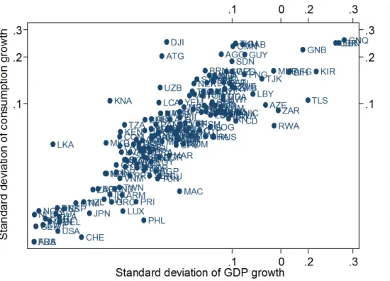
Before proceeding, we should emphasize that we focus the analysis on GDP volatility because for most countries in the world, GDP and consumption ‡uctuations are almost perfectly correlated. Hence, accounting for GDP volatility goes a long way in accounting
for consumption volatility (see Figures 1 and 2).3 Accordingly, in the modeling section, we abstract from …nancial trade in assets.4
The remainder of the paper is organized as follows. Section II reviews the literature. Section III presents the model and solves analytically for two special cases, autarky and costless free trade. Section IV introduces the data, calibration, and quantitative results. Section V presents concluding remarks. The Appendix contains further derivations and a detailed description of the datasets used in the paper.
Figure 1: Volatility (standard deviation ) of Annual per capita GDP Growth and Annual per capita Consumption Growth. The data come from the World Bank’s World Development Indicators 1970–2007.
3Figure 1 shows the volatilities of per capita consumption and GDP. Figure 2 shows the volatilities of
aggregate consumption and GDP.
4There is an obvious analogy between diversi…cation through trade in goods and diversi…cation through
trade in …nancial assets. However, trade in assets stabilizes consumption, not GDP (indeed, trade in assets might increase GDP volatility, as capital would tend to ‡ow to high productivity countries and amplify productivity shocks), whereas in contrast, trade in goods stabilizes GDP— and as a by-product, also con-sumption. Given the patterns in Figure 1, there appears to be limited asset diversi…cation across countries.
Figure 2: Volatility (standard deviation) of Aggregate Annual GDP Growth and Aggregate Annual Consumption Growth. The data come from the World Bank’s World Development Indicators 1970–2007.
II
Literature Review
A number of empirical studies have exploited variation across countries to study the e¤ects of trade openness on volatility. Some studies, most notably Rodrik (1998), Easterly, Islam, and Stiglitz (2000), Kose, Prasad, and Terrones (2003) …nd that trade openness increases volatility, while others, including Haddad, Lim and Saborowski (2010), Cavallo (2008), and Bejan (2006) …nd that trade openness decreases volatility. Di Giovanni and Levchenko exploit variation across countries and across sectors, concluding that trade openness leads to higher volatility. Strotmann, Döpke, and Buch (2006) exploit variation across …rms in
Germany and infer that exposure to international trade increases …rm-level and aggregate volatility. While the use of sector- or …rm-level data allows researchers to control for a number of country-speci…c determinants of volatility, omitted-variable biases at lower levels of aggregation, reverse causality, and possibly heterogenous e¤ects of trade openness across countries remain important concerns.5
To understand the causal e¤ect of trade openness on volatility, we build on a variation of the theoretical model formulated by Eaton and Kortum (2002), further extended by Alvarez and Lucas (2006) and Caliendo and Parro (2012). The model is amenable to quantitative calibration and has proven useful at replicating trade ‡ows and production patterns across countries. Variations of this model have been used to address a number of questions in international economics— questions related to the e¤ects of trade on the “…rst moments” of domestic or foreign productivity, but not the trade e¤ects on countries’aggregate volatility. For example, Hsieh and Ossa (2011) study the spillover e¤ects of China’s growth on other countries; di Giovanni, Levchenko, and Zhang (2014) study the global welfare impact of China’s trade integration and technological change; Levchenko and Zhang (2013) investigate the impact of trade with emerging countries on labour markets; Burstein and Vogel (2012) and Parro (2013) study the e¤ect of international trade on the skill premium; Caliendo, Rossi-Hansberg, Parro, and Sarte (2013) study the impact of regional productivity changes on the U.S. economy, and so on. None of these applications, however, focuses on the impact of openness to trade on volatility. The closest paper to ours, both on question and mod-elling framework, is Burgess and Donaldson (2012), who use the Eaton-Kortum model in 5Trade is by no means the only determinant of volatility. For studies of other determinants of volatility,
see Kose, Prasad, and Terrones (2003), Raddatz (2006), Koren and Tenreyro (2007, 2011, 2013), Berrie, Bonomo and Carvalho (2013), and the references therein.
conjunction with data on the expansion of railroads across regions in India to assess whether real income became more or less sensitive to rainfall shocks, as India’s regions became more open to trade. The authors …nd that the decline in transportation costs lowered the impact of productivity shocks on real income, implying a reduction in volatility. Our analysis high-lights that, while a reduction in volatility has been experienced by many countries as they became more open to trade, the size and sign of the trade e¤ect on volatility may be— and indeed has been— di¤erent across di¤erent countries.6;7
Our results also relate to Wacziarg and Wallack (2004), who empirically study 25 episodes of trade liberalizations and …nd a relatively small extent of labour reallocation across sec-tors. Though the authors do not analyze volatility patterns, their results are consistent with our …nding that, on average, the sectoral-specialization channel tends to be of limited quantitative importance; our results, however, point out to signi…cant heterogeneity in the e¤ects, indicating that the sectoral specialization channel played an important role in certain countries, most notably Italy and the Netherlands.
Our paper is also related to the seminal contribution of Backus, Kehoe, and Kydland (1992). The authors show that in a real-business-cycle setting, GDP volatility is higher in the open economy than in the closed economy, as capital inputs are allocated to production in the country with the most favorable technology shock. In other words, GDP ‡uctuations are ampli…ed in an open economy. (In contrast, consumption volatility decreases in the 6Though similar in question and modelling framework, the quantiative approach carried out in our paper
is very di¤erent from that adopted for India by Burgess and Donaldson (2012).
7See also Donaldson (2015), where the question also is addressed in the context of India’s railroad
ex-pansion. There is also a growing literature on the e¤ect of globalization on income risk and inequality. We do not focus on distributional e¤ects within countries in this paper, though it is obviously a very important issue, and a natural next step in our research. For theoretical developments in that area, see for example,
open economy, as …nancial markets allow countries to smooth the impact of GDP shocks on consumption; this result generates a large cross-country correlation of consumption relative to the cross-country correlation of output, which, as the authors point out, is not borne out by the data.) In our multi-country, multi-sector setting, instead, GDP volatility can— and often does— decrease with openness, as intra-temporal trade in inputs allows countries with less favorable productivity shocks to source inputs from abroad, thus reducing GDP (as well as consumption) volatility.8 Also related is the empirical literature initiated by Frankel and Rose (1998), who documented a strong correlation between bilateral trade ‡ows and GDP comovements between pairs of countries. Our main focus in this paper is on thecausal e¤ect of trade onvolatility— and the channels mediating this e¤ect— but the quantitative approach we follow in our counterfactual exercise can potentially be extended to also identify thecausal
e¤ect of trade on bilateral comovement— and indeed, other higher-order moments. We keep the focus on volatility, which is our main motivation, and speak to the perennial question of how trade might a¤ect it.9
Readers of Kehoe and Ruhl (2008) may wonder whether changes in terms of trade caused by (broadly construed) foreign productivity shocks a¤ect measured real GDP— and hence real GDP volatility. In the Appendix we explain that this is indeed the case, given the way in which statistical o¢ ces construct real GDP measures in practice.
8A number of papers have tried to address the comovement “anomaly” pointed out by Backus, Kehoe,
and Kydland (1992), that is, the result that cross-country consumption correlations increase vis-à-vis cross output correlations in the open economy; see, for example, Stockman and Tesar (1995). In this paper, we focus on the e¤ect of trade on output volatility and refer readers interested in the comovement puzzle to the complementary literature.
9For studies on the e¤ect of bilateral trade on bilateral comovement, see Kose and Yi (2001), Arkolakis
III
A Model of Trade with Stochastic Shocks
The baseline model builds on a multi-sector variation of Eaton and Kortum (2002), Alvarez and Lucas (2006), and Caliendo and Parro (2012), augmented to allow for stochastic shocks, as well as frictions to the allocation of non-produced (and non-traded) inputs across sectors.
A
Model Assumptions
The world economy is composed ofN countries. At a given point in timet, each countrynis
endowed with Lnt units of a primary (non produced) input, which we interpret as equipped
labour. There are J sectors (or broad classes of goods) in the economy, whose output is
combined into a …nal good through a Cobb-Douglas aggregate. In formulas, aggregate gross output in the economy is given by:
Qnt = J Y j=1 Qjnt j (1)
where Qjt is the gross output in sectorj and PJj=1 j = 1. Competitive …rms in each sector
j produce a composite good according to the following constant-elasticity-of-substitution
(CES) technology: Qjnt = Z 1 0 qnt(!j) 1 d!j 1 (2)
whereqnt(!j)is the quantity of good!j used by countrynin sectorj at timet, and >0is
the elasticity of substitution across goods within a given sector. The intermediate goods !j
m; we assume that jmnt jmkt jknt 8m; n; k; j; t and jnnt = 1. All costs incurred are net
losses.10 Under the assumption of perfect competition, goods are sourced from the lowest-cost producer, after adjusting for transport lowest-costs. The technology for producing qnt(!j) is
given accordingly by the country of origin (m) with the lowest cost (with m = n when the
good is produced locally):
xmt(!j) =Ajmtzm(!j)lmt(!j)
j
Mmt(!j)1
j
(3)
where xmt(!j) is the production of good!j by countrym at timet,Mmt(!j)is the amount
of the aggregate composite good used by countrym to producexmt(!j)units of good !j and
lmt(!j) is the corresponding amount of equipped labour. Total factor productivity (TFP)
levels vary across countries, sectors, and goods. Speci…cally, each intermediate good !j in
sectorj of countrynhas a time-invariant idiosyncratic productivity factorzn(!j)and a
time-varying factor Ajnt common to all the goods !j in sector j. Building on the literature, we
assume the productivitieszn(!j)follow a sector-speci…c, time-invariant Fréchet distribution
Fj
n(z) = exp( Tnjz ). A higher Tnj shifts the distribution of productivities to the right, that is leading to probabilistically higher productivities. A higher decreases the dispersion of the productivity distribution, and hence reduces the scope for comparative advantage. Shocks toAjnt over time are interpreted as standard sectoral total factor productivity (TFP)
shocks.
The single …nal good can be used both as input in the production of intermediaries !j 10In the calibration, the s will re‡ect all trading costs, including tari¤s; so implicitly we adopt the
extreme assumption that tari¤ revenues are wasted— or at least not rebated back to agents in a way that would interact with the allocation of resources in the economy.
or for …nal consumption, Cnt. Hence, market clearing in the good markets implies: Qnt =Cnt+ J X j=1 Z 1 0 Mnt(!j)d!j;
where the integral aggregates over the unit-size continuum of goods!j entering in the
pro-duction of each sector’sj aggregate good.
Clearing in the input market within a sector implies:
Ljnt = Z 1
0
lnt(!j)d!j;
where lnt(!j) denotes the amount of equipped labour used in the production of good!j by
country n. The (equipped) labour allocated to each sector, Ljnt; with PJk=1Lk
nt = Lnt, are determined ex ante (before the realization of the shocks). Speci…cally, we assume there is perfect risk-sharing within a country, but no risk-sharing across countries.11 At the beginning of each period, a representative consumer decides on the optimal allocation of the primary input Lnt into di¤erent sectors in order to maximize the expected value of utility; then
(stochastic) shocks to productivity Ajnt are realized, equipped labour is reallocated within
a sector (but not across sectors), and production and consumption take place. The lack of ex-post reallocation across sectors in a given period aims at capturing the idea that in the short run, it is costly to reallocate productive factors across sectors. Hence, ex post, Ljt is
…xed until t+ 1:12
11To motivate the lack of risk-sharing across countries, see our discussion of Figures 1 and 2.
12In the quanti…cation, a period will be one year. This amounts to assuming that it takes at least one
The representative consumer’s budget constraint in each period is: PntCnt = J X j=1 wntj Ljnt;
wherePnt is the price of the aggregate good (1),w j ntL
j
ntis the nominal value-added generated in sectorj. Lifetime utility is given by
Un= 1 X t=0 tu(C nt);
where u0 > 0, u00 0 and is the discount factor. Because there is no intertemporal
trade and no capital in the economy, each period consumers maximize the expected static utility ‡ow E[u(Cnt)] and the equilibrium is simply a sequence of static equilibria (in the
quantitative section, we allow for trade imbalances). In making his labor allocation decisions the representative consumer takes into account the joint probability distribution function of sectoral productivities, Ajnts.
In the analysis, we assume log utility and therefore the consumer solves:
Ljnt = arg maxEt 1 " ln PJ j=1w j ntL j nt Pnt !# ; s:t::XJ j=1L j nt =Lnt; (4)
where Et 1 indicates that the expectation is taken before the realization of period t shocks.
This maximization problem leads to the following …rst-order conditions for the allocation of inputs to sectors: Ljnt Lnt =Et 1 " wjntLjnt P kw k ntLknt # ; 8j; t: (5)
In words, the share of resources allocated to a given sector equals its expected share in value added. To gain intuition on this expression note that1=PkwkntLknt is the marginal utility of consumption in period t; thus, more resources are allocated to higher value-added sectors,
after appropriately weighting by marginal utility. Consider, for further intuition, a (small) sector whose productivity is negatively correlated with the rest of the economy (that is, it has high value added when the rest of the economy has low value added); in states of the world in which overall income is low, the marginal utility of consumption 1=Pkwk
ntLknt will be high and hence the optimal allocation entails allocating more resources to this sector. (Log-linearizing this expression makes the role of second moments on the allocation of resources clearer.) In the closed economy, the value-added share is pinned down by the Cobb–Douglas coe¢ cients j j, as with Cobb-Douglas technology there is no variation on expenditures
(and sales) shares— and log-utility implies the shares determine the sectoral allocation of resources. (In the open economy this result no longer holds as a country’s sectoral shares depend on its absolute and comparative advantage as well as trading costs vis-à-vis other countries.
B
Model Solution
We …rst discuss the solution under autarky, and then turn to the solution under free trade.
Solution under Autarky We solve the model backwards in two stages. First, we solve
the model taking the sectoral allocation of nonproduced inputs Ljt as …xed. We then solve
The demand for each sector’s composite good is given by Qjt = jt P j t Pt ! 1 Qt; (6)
and the demand for each intermediate good !j is
qt(!j) = pt(!j) Ptj Q j t; where Ptj = Z 1 0 pt(!j)1 d!j 1 1 (7)
is the aggregate price index in sectorj, and the economy-wide price index is given by:
Pt= J Y j=1 j jt t P j t j t : (8)
The demand for non-produced inputs lt(!j) and produced inputs Mt(!j) are given,
respec-tively, by ljt(!j) = j pt(!j)qt(!j)
wtj
and Mt(!j) = (1 j)pt(!
j)q t(!j)
Pt : Aggregating over all goods
!j in a given sector, we obtain
wjtLjt = jPtjQjt (9)
and, correspondingly,PtMtj = (1
j)Pj tQ
j
t:Using the input demand functions and the zero pro…t condition the autarky prices of intermediate goods are given by:
pt(!j) =Bj Ajt z(!j)
1 wtj
j
whereBj = j j
(1 j) (1 j). Using (10) and the properties of the Fréchet distribution,
we can express the sectoral price index as:
Ptj = BjhAjt Tj
1i 1
wjt
j
Pt1 j (11)
where = +1 ;and is the gamma function. Using (6), (9), and (8) we obtain real GDP: Yt= J X j=1 wtjLjt Pt = J Y j=1 Rj Ajt j Ljt j j ; (12) where = PJj=1 j j and R j /QJj=1 j j j j (Bj) j (Tj) j is a time-invariant prod-uct.
We can now move one step backward and solve for the allocation of the primary input across sectors, Ljt; j = 1; :::; J. From (4) and (5), Ljt = j jLt.13 Substituting into (12), GDP is given by: Yt= J Y j=1 Rj j j j j Ajt j Lt (13)
In words, GDP varies with ‡uctuations in sectoral productivity,Ajt, and aggregate resources,
Lt:
Solution with International Trade The key di¤erence in the internationally open
econ-omy is that inputs can potentially be sourced from di¤erent countries. Delivering a unit of 13The FOC are j jE[u0(Ct)Ct] = Lj
good !j produced in countrym to countryn costs: pjnmt(!j) = B j wj mt j Pmt1 j Ajmt jnmtzm(!j) whereBj wmtj j
Pmt1 j is the cost of the input bundle in country of originm, sectorj, at time
t. Because of perfect competition, the price paid in country n, denotedpnt(!j), will be the
minimum price across allN potential trading partners: pjnt(!j) = min pj
nmt(!j); m = 1; :::; N : Producers of the aggregate good in (1) minimize production costs taking prices as given. We assume the distribution of e¢ ciencies for any good !j in sector j and country n are
independent across countries and sectors and follow a time-invariant Fréchet distribution:
Fnj(z) = exp( Tnjz ): Under this assumption, the distribution of prices in sectorj of
coun-tryn, conditional on Ajmt m=1;:::N is given byGjnt(p)jfAj
tg= Pr(P j nt < p) = 1 exp j ntp where jnt = PNm=1Tj m Bj(wj mt) j Pmt1 j Ajmt jnmt !
. Given that there is a continuum of !j in each
sector, by the law of large numbers the probability that country mprovides a good in sector
j at the lowest price in country n equals the fraction of goods that country n buys from
countrym in sectorj: djnmt= Tj m Bj(wj mt) j Pmt1 j Ajmt j nmt ! j nt (14)
that is, djnmt is the fraction of countryn’s total spending on sector-j goods from country m
at timet. The equilibrium in the open economy can be de…ned as following.
Equilibrium De…nition. An equilibrium in the open economy is de…ned as a set
of resource allocations Ljnt , import shares djnit , prices fPntg, Pntj , and fwjng such
that, given technology Ajit ; Titj ;aggregate endowments fLntg and trading costs j int
i)consumers maximize expected utility, ii) …rms minimize costs and,iii)markets for goods
and inputs clear, and iv) trade is balanced. In equilibrium, prices and quantities satisfy
(15)-(21): Pnt = J Y j 1 j n j Pntj j (15) Pntj = jnt1= (16) j nt = B j N X i=1 Tij Ajit 2 4P 1 j it w j it j j nit 3 5 (17) djnmt= (Bj) Tmj Ajmt P 1 j mt w j j mt j nmt j nt ; N X m=1 djnmt= 1 (18) wntj Ljnt = j N X m=1 djmnt " j +1 j j wmtj Ljmt wmtLmt # wmtLmt (19) wntLnt = J X j=1 wjntLjnt (20) Ljnt Lnt =Et 1 " wntj Ljnt PJ k=1w k ntLknt # (21)
Equations (15)–(17) show the equilibrium prices as a function of technology and input costs resulting from …rms’cost minimization and consumers’maximization problems. The …rst equation in (18) shows the value of goods from sector j bought by country n from
country m as a share of total spending on goods j by country n: The second equation says
that the sum of spending shares on goods j from all countries m by country n (including n
itself) add to 1, that is, imports plus domestic expenditures on goodsj by countryn, add up
sales accruing to the primitive factor in sector j of country n; it already incorporates the
balanced trade condition, i.e., total payments for goods ‡owing out of countrym to the rest
of the world equal payments ‡owing in countrymfrom the rest of the world.14 Equation (18) expresses total value added in the economy as the sum of sectoral value added. (Real value added is given byYnt = wntPntLnt.) Finally, (21) expresses the resource shares as a function of
expected shares, following the …rst order conditions in (5).
The model can conceptually be solved backwards in two steps. First, for any given set of values for Ljnt, the …rst …ve sets of equations can be solved for Pnt, wntj , Pntj , djnmt as a
function of the jmnts and the augmented productivity factors de…ned as:
Zntj TnjhLnt Ajnt
1= ji
j
: (22)
Then in a …rst stage, we can solve for the shares Ljnt
Lnt. As seen, with log utility the solution
for Ljn
Ln simpli…es signi…cantly as it is the expected value of sectoral value-added shares; in
the implementation, we will use the data to help pin down these expectations.
C
Two Illustrative Cases: Autarky and Costless Trade
To illustrate the mechanism of diversi…cation through trade, we analyze a one-sector version of the model (that is, the Eaton-Kortum model) under two extreme cases for which we have closed-form analytical solutions for GDP: autarky and costless trade. We accordingly drop
14In formulas,PJ j=1X j mt= PN n=1 PJ j=1d j nmtX j nt, whereX j
ntis total expenditure by countrynon sector-j goods. The right-hand side is the total demand by all N countries for goods produced in countrym. The left-hand side is the total expenditures by countrym, which, under trade balance also equals its total sales. Recall that PmjQjm is the total purchases of goods from sector j by country m: Note Pmtj Qjmt, the total purchases of goods from sectorj by countrym: Hence: Pmtj Qjmt= jw
mtLmt+1 j j w j mtL j mt.
the sector subscripts.
C.1 Volatility under Autarky
Under complete autarky, value added in the one-sector economy is given by (13), which can be rewritten as:
Ynt /(Znt)
1
where Znt Tn LntA
1=
nt . Taking log-di¤erences around the mean (or trend value in the empirics), we obtain,
^
Ynt = 1 ^Znt:
Thus, in the one-sector economy under autarky, shocks to value added are driven exclusively by domestic shocks to the productive capacity of the economy, Z^nt: The variance of GDP,
V( ^Ynt) thus depends on the variance of the shocksV( ^Znt):
V( ^Ynt) = 1
( )2V( ^Znt):
C.2 Volatility under Costless Trade
Under costless trade in the one-sector economy ( nmt= 1), GDP per capita simpli…es to:15
Ynt = ( B) 1= Z 1 1+ nt N X m=1 Z 1 1+ mt !1
and hence GDP ‡uctuations are given by: ^ Ynt = 1 1 + " ^ Zn+ 1 XN m=1 mZ^m # where m = Z 1 1+ m PN i=1Z 1 1+ i
is the relative size of country j evaluated at the mean ofZjs.
Rear-ranging, we obtain: ^ Ynt = 1 " n+ 1 + Z^n+ 1 1 + N X m6=n mZ^m # (23)
Volatility under free trade is hence given by:
V ar( ^Ynt) = 1 2 8 > > < > > : n+ 1+ 2 V ar( ^Znt) + h 1 1+ i2P m6=i 2 mV ar( ^Zmt) 2 n+ 1+ 1 1+ P m6=n mCov( ^Zm;Z^n) 9 > > = > > ; (24)
Compared to the variance in autarky, V( ^Ynt) = ( 1)2V( ^Znt), it is clear that the volatility due to domestic productivity ‡uctuations, V ar( ^Znt); now receives a smaller loading, as
n+
1+ 2
< 1 since n < 1: The smaller the country (as gauged by its share n), the
smaller the impact of domestic volatility of shocks, Z^n; on its GDP, when compared to
autarky. Openness to trade, however, exposes the economy to other countries’productivity shocks, which will also contribute to the country’s overall volatility. Whether or not the gain in diversi…cation (given by lower exposure to domestic productivity) is bigger than the increased exposure to new shocks depends on the variance-covariance matrix of shocks across countries. If all countries have the same constant variance V ar( ^Znt) = ; and the Z^nt are
uncorrelated, volatility under free trade becomes: V ar( ^Ynt) = 1 2( n+ 1 + 2 + 1 1 + 2X m6=i 2 m ) (25)
which is unambiguously lower than the volatility in autarky given that16
n+ 1 + 2 + 1 1 + 2X m6=i 2 m <1 (26) (recall m <1and PNm=1 2
m 1). Of course, if other countries have higher variances or the covariance terms are important, then the weights countries receive matter and the resulting change in volatility cannot be unambiguously signed.
IV
Mapping the Model into Observables
In this section, we connect the model to the data and use it to quantitatively assess the e¤ect of historical changes in trade barriers on GDP volatility for a diverse sample of 24 core countries and an aggregate of the remaining countries to which we refer as “rest of the world” (ROW).
The equilibrium of the model is characterized by equations (15)-(21). We solve the model numerically, for which we need to calibrate the values of the exogenous trading costs jnmt,
the productivity process Zntj , and the parameters j, j, , and . We consider 24 sectors 16since( )2 + 2 n+Pj=1 2 j <(1 + )2as 2 n+X j=1 2 j<2 + 1
in the analysis (agriculture, 22 manufacturing sectors, and services). Throughout the study, services are treated as a nontradable sector (that is, jnmt = 0 for all n 6= m and
j
nmt = 1 forn =m), whereas agriculture and all manufacturing sectors are treated as tradables, with
potentially di¤erent trading costs.
We set j so as to match the average share of each sector on total …nal uses in the OECD
Input-Output tables across all countries. The betas for each sector are calculated as the ratio of value added to total output. A detailed description of the data and the calculations are available in the Appendix.
We allow for a relatively broad parametric range for , from = 2 to = 8; consistent
with the estimates in the literature (see Eaton and Kortum, 2003, Donaldson 2015, and Simonovska and Waugh, 2011). We use = 4 as the baseline case, and report the results for other values when discussing the sensitivity of our results. We calibrate the elasticity of substitution across varieties = 2, consistent with Broda and Weinstein (2006). The results are not sensitive to this parametric choice.
We explain next how we obtain the processes for jnmt and Z j
it using data on sectoral bilateral trade ‡ows, value added, output, and prices. Before we specify the details, a quick intuition on how these series are backed-out from the model is as follows. We recover trade costs jnmt using information on bilateral trade shares and gross output at the sectoral
level. Intuitively, if two countries trade little with one another in a given sector (relative to the sectoral gross output of these countries), this will signal high trade costs between the countries in that sector. Second, we recover productivities relative to a benchmark country using the market share of each exporter. If a country has a high export share in a sector, that is a sign of revealed comparative advantage, meaning a high relative productivity in the
sector relative to the benchmark country. To calibrate the absolute level of productivities, we use price data for a benchmark country. We explain the procedure in detail and with formulas in the next section.
A
Implementation
Kappas In order to perform counterfactual experiments we need to back out the historical realizations of the exogenous processes. Following the idea in Head and Ries (2011), we assume that sectoral bilateral trading costs are symmetric, that is: jnmt = jmnt, and hence
bilateral trade costs at the sectoral level can be backed out from the data. Indeed, inverting the structural model, we obtain:
djnmtdjmnt djmmtdjnnt = j nmt 2 : (27)
The left hand side objects can be measured using data on bilateral imports and gross output at the sectoral level. Speci…cally, djnmt is the value of exports from m to n in sector j at t
relative to total spending by n on sector j at time t, where total spending is measured as
gross output plus imports minus exports by that sector and country at time t: The share
djmmt is obtained as a residual from the accounting restriction:
djmmt = 1 N X n6=m
djmnt
Hence, for a given value of , we can obtain the time series of trading costs by sector and country-pairs j .
Productivity in Tradable Sectors To back out the productivities, we proceed as follows. First, using the formula for djnm in equation (18), after some algebra, we obtain:
djnm = (B j) j m j Zmj ( jnm) (ymj ) j Pm jn , (28) where jm Ljm Lm and y j m Ljmwjm
Pm . We can exploit this to recoverZ
j m:In particular, inverting (28) we have: Zmtj =Bj djnmt ymj j j nmt Pntj Pmt ! j mt j (29)
To approximate terms on the right hand side we use data on sectoral import shares djnmt,
sectoral value added yj
m, sectoral shares j
mt, and aggregate prices Pnt along with the cal-ibrated parameters. (See the Appendix for more details.) The only terms we cannot back out directly from data are sectoral prices. We thus use the model in conjunction with the data to infer them. Note …rst that equation (29) holds for all (n; k) pairs of countries and
all sectors j (except for services). The procedure becomes clear when we collect known and
unknown terms as follows:
Zntj = Bj dk;n;tj jk;n;t wn;tj Ljn;t j j n;t j Pn;t (1 j) | {z } exp( jk;n;t) Pk;tj = exp( jk;n;t)Pk;tj (30)
Note in particular that this relationship holds for any choice of country k. Note also that
the factor exp( jk;n;t) can be constructed from observable data. We decompose exp( jk;n;t) =
1. Take logs and rename terms for brevity. j k;n;t = lnZ j nt+ lnP j k;t (31) j nt+ j k;t (32) where jnt lnZntj and jk;t lnPk;tj .
2. To proceed we need a benchmark country, so we use sectoral prices in the US.
j
U S;t lnP j U S;t
We choose units of accounts for each sector so that U.S. nominal sectoral prices are equal to 1 in 1972.
3. Obtain jk;t for all other countries as:
j k;t = 1 N N X n=1 j k;n;t j U S;n;t + j U S;t (33)
(Note that this equation holds with and without the averaging operator, N1 PNn=1, as j
k;t and j
U S;t do not depend on the exporter n. 17)
4. Back-out jnt for all other countries:
j nt = 1 N N X k=1 j k;n;t j k;t (34)
5. Recover shocks and prices: Zn;tj = exp jnt (35) Pk;tj = exp j kt ! (36)
At the end of the procedure we end up with augmented productivity factors Zn;tj and
sectoral prices for agriculture and all manufacturing sectors Pk;tj .
Productivity in Nontradables To compute the productivities in the services sector for
each country, we use equilibrium equations (15), (16) and (28).
1. As we already have sectoral prices of tradables we can use (15) to recover the price of services as follows: Pn;ts = Pn;t PU S;t PU S;t 1 s YJ j=1 j j ! 1 s " Y j6=s Pn;tj j # 1 s (37)
Note that we observe data on the price of countryn relative to the price in the United
States, Pn;t
PU S;t, from the Penn World Tables.
2. Now we recover Zn;ts using (16), (28), and n =m.
Zn;ts = Bs w s n;tLsn;t s n;t s Pn;t PU S;t PU S;t (1 s) Pn;ts (38)
Sectoral versus Aggregate Shocks Note that the changes in productivity retrieved above, 1 j Z^ j m 1 jA^ j mt+ ^Lmt; (39)
can be decompose into two factors: a sectoral factor, 1jA^
j
mt, and an aggregate factorL^mt. The interpretation ofLmt as “equipped labour”means that it embeds a productivity component
too. Given the functional form, the split between pure productivity and resources in Lmt
is not relevant from the point of view of aggregate volatility. (A shock to Lmt will be
equivalent to an aggregate shock to Ajmts that leaves the relative productivities Ajmt=Ajmt0
unchanged8j; j0:) For identi…cation, we impose the restriction that
X j
jA^ j
mt= 0: (40)
Thus, changes in the sectoral productivity will correspond to changes in the relative value of Ajmt, while changes in aggregate productivity (a¤ecting all sectors equally), as well as
changes in overall resources, will be subsumed in Lmt. We hence call sectoral shocks, those
a¤ecting A^jmt and aggregate shocks those a¤ecting the aggregate factor L^mt. The
identi-…cation restriction implies that any primitive aggregate shock a¤ecting all sectors will be collected in L^mt:
Summary of the Procedure We can summarize the procedure as follows.
1. Obtain the inverse of trade costs, s, from (27). j
3. Retrieve the panel of sectoral and country productivities Zmtj from the procedure
described above.18
4. Retrieve Lmt from (39) using (40) and compute Ljmt= j mtLmt:
5. Solve the equilibrium values of djnit , fPntg, Pntj , and fwnjg using equations (15)
through (20).
A.1 Counterfactual Equilibria
We discuss next how we compute the equilibrium in the counterfactual exercise and how we identify the two theoretical mechanisms.
Numerical Counterfactual Equilibria For each new value of (inverse) trading cost ,
and the estimated sequence of sectoral productivities Zmtj , we need to solve for the sequence
of equipped labour allocated to each sector Ljmt . The rational-expectations equilibrium is
a …xed point of a below mapping on the space of all possible sequences Ljmt . We proceed
as follows.
1. We start from the initial value (Ljnt)0 = jLnt.
2. In iteration i for the actual (Ljnt)i we get sectoral and aggregate (equipped labour)
wages, (wntj )i and (wnt)i, from the equilibrium equations.
3. We calculate the implied total value added and the sectoral value added shares as
wjntLjnt wntLnt !i = (w j nt)i(L j nt)i (wnt)iLnt :
4. (a) Decompose all N J value-added-share series into trend and cycle components
using an annual band-pass …lter.
log w j ntL j nt wntLnt !i =trendjnt+cyclejnt:
(b) Normalize the trend values so that in each period and each country the trend values add up to 1: \ wjntLjnt wntLnt !i = exp(trend j nt) P kexp(trendknt)
(c) Replace the expectation with the adjusted trend value.
Et 1 wjntLjnt wntLnt ! = \ wjntLjnt wntLnt !i
5. Update the resource allocations
(Ljnt)i+1 =Lnt
\
wjntLjnt wntLnt
!i
6. Repeat the procedure until convergence.
Productivities in Counterfactual Scenario We are interested in decomposing the trade
e¤ect on volatility on the contributions of the two mechanisms, specialization and diversi…-cation. To achieve that, we need to identify the sources of shocks to productivity. We resort to a factor model that decomposes productivity shocks into sector- and country-speci…c
com-from trends we use a band pass …lter to detrend each logZn;tj T
t=1 series. Then we calculate
the time average of the shocks for each (n; j) pair and subtract it from the growth rate to
get the object to be decomposed, Z~ntj .
~ Zntj = ^Zn;tj (T 1) 1 T X t=2 ^ Zn;tj
Without loss of generality, we decompose Z~ntj as:
~
Zntj = jt + nt+ jnt;
where n;t is the country-speci…c factor, a¤ecting all sectors within the country; j
t is the global sectoral factor, a¤ecting sector j in all countries; and the residual jn;t is the
idio-syncratic component, speci…c to the country and sector. The three factors, ; , and are
estimated as: ^j t =N 1 N X n=1 ~ Zntj ^nt =J 1 J X j=1 ~ Zntj ^jt ^jnt = ~Zntj ^jt ^nt,
with the restrictionPn n= 0 implying that the country-speci…c e¤ect is expressed relative to the world’s aggregate. In the counterfactual exercises, we can mute the sector- or country-speci…c factors by setting the corresponding components equal to 0, in order to identify the separate e¤ects of the two trade channels a¤ecting volatility.
V
Quantifying the E¤ect of Trade on Volatility
This section uses the framework developed above to quantitatively assess how historical changes in trade costs from the early 1970s have a¤ected volatility patterns in a sample of countries at di¤erent levels of development.
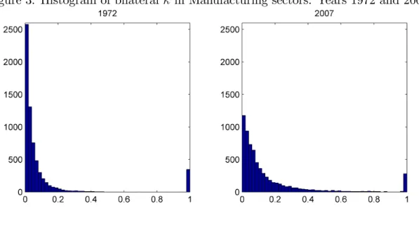
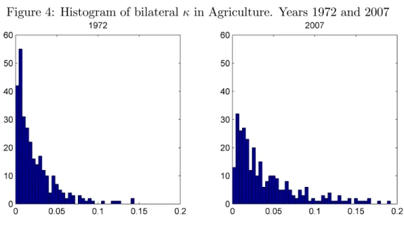
Trade barriers have declined signi…cantly since the early 1970s. This decline in barriers (or increase in ) is illustrated in Figures 3and 4, which show, correspondingly, the histograms of bilateral s in manufacturing and agriculture in the …rst and last year of our sample. As the …gures show, the distribution of has moved to the right, indicating a decline in trading costs in both sectors.
Figure 4: Histogram of bilateral in Agriculture. Years 1972 and 2007
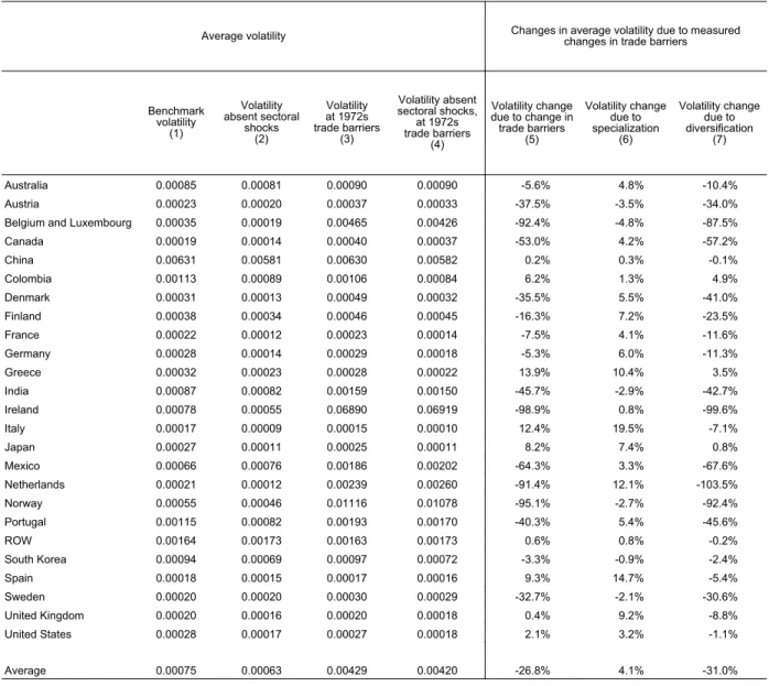
Table 1 investigates how the changes in trading costs have a¤ected volatility in the 25 countries in our sample. (The list of countries can be seen in Table 1.) The results in the table correspond to our benchmark calibration, based on = 4: Column (1) in the
table shows the volatility generated by the model. Volatility is computed as the variance of annual growth rates over 35 years (we focus on the variance rather than the standard deviation, as the variance allows for an additive decomposition into the two mechanisms we are interested in). The value reported in Column (1) is very close to the actual volatility experienced by these economies from 1972 through 2007, since both the trading costs and productivity processes fed into the model are backed out from the data. Column (2) shows the volatility that would be observed if there were no global sectoral shocks. (The latter is generally smaller than the benchmark volatility, though there are some exceptions, as global sectoral shocks can covary negatively with country-speci…c shocks in some countries.) To compute this counterfactual measure, we mute the global sector-speci…c shocks in the decomposition of Z~ntj . (This measure of volatility is useful to identify and quantify the two
trade channels, as it will become clear next.) Column (3) shows the country’s volatility in the counterfactual scenario that trading costs ( ) stayed at their 1972 levels. Column (4) shows this latter measure in the absence of global sector-speci…c shocks.
Column (5) shows the percent change in average volatility due to actual changes in trading costs since 1972, that is, the percent di¤erence between columns (1) and (3). Column (6) shows the contribution of the specialization channel to the change in volatility in (5) and Column (7) shows the corresponding contribution of the diversi…cation channel. The contribution of diversi…cation to the change in volatility is computed as the di¤erence between the volatility in the absence of sectoral shocks (Column 2) and the volatility under 1970’s trading costs, in the absence of sectoral shocks (Column 4); the di¤erence is expressed relative to the volatility under the 1972’s trading cost levels (Column 3). This measures captures the trade in volatility due exclusively to the country-diversi…cation e¤ect, as the sectoral shocks are muted. The volatility due to specialization is computed as the di¤erence between Columns (5) and (7).
As Table 1 shows, two thirds of the countries in our sample experienced a decline in volatility due to the decline in trade barriers since 1972, while the other third of the countries experienced an increase in volatility. The biggest decreases in volatility caused by trade occurred in Belgium-Luxemburg, Ireland, the Netherlands, and Norway, all of which saw volatility reductions of over 90 percent, meaning their current volatility is 90 percent lower than it would have been if trading costs stayed at their 1972 levels. The biggest increases in volatility due to trade were witnessed by Greece (14 percent increase) and Italy (12 percent increase). These results are the net e¤ect stemming from the contribution of the two separate
percent of the countries. The specialization channel contributed to increase volatility in two-thirds of the countries, with the biggest increases experienced by Italy, Spain, the Netherlands and Greece. In some countries, sectoral specialization actually contributed to lower volatility; this is the case of Austria, Belgium-Luxembourg, India, Norway, South Korea, and Sweden. This is possible, as the model illustrates, when the sector (or sectors) in which the economy specializes in comoves negatively (or less positively) with the country’s aggregate shocks— or other sectoral shocks. Interestingly, the United Kingdom did not experience a sizeable change in its volatility due to changes in trade costs. However, this result masks the contribution of a sizeable reduction in volatility due to the diversi…cation channel and a comparably sizeable increase in volatility due to the sectoral specialization channel.
In absolute terms, the diversi…cation e¤ect was in general larger than the specialization e¤ect, and hence, on net, two-thirds of the countries saw a reduction in volatility, while the remaining third saw a more modest increase in volatility. The heterogeneity in the trade e¤ects across countries is remarkable.
Table2shows the change in volatility due to free trade and its decomposition for two other (more extreme) values of , = 2 and = 8: The general message is qualitatively robust: i)
the e¤ect of trade on volatility varies across countries; ii) the diversi…cation channel tends to reduce volatility; and iii) sectoral specialization tends to increase volatility. Interestingly, for = 2, the case of high scope for comparative advantage, volatility always declines with trading costs, with the declines being signi…cant even for countries like the United States. The decline in volatility is driven almost exclusively by the large e¤ects stemming from the country-wide diversi…cation channel. The e¤ects of sectoral specialization are also sizeable, but smaller than the diversi…cation e¤ect. These results imply that, on average, trade leads
to a reduction in volatility. On the other extreme of = 8, the results are qualitatively similar to the benchmark case, although in general the results are quantitatively smaller. Taken together, the …ndings appear robust to increases in and suggest that the e¤ect of country diversi…cation on volatility would be stronger for lower values of , meaning that trade will reduce volatility even further as the scope for comparative advantage increases. (This result holds despite the fact that sectoral specialization would also increase in this case.)19
VI
Conclusions
How does openness to trade a¤ect GDP volatility? This paper revisits the common wisdom that trade increases volatility by causing higher sectoral specialization. It argues that when country-speci…c shocks are an important source of volatility, openness to international trade can lower GDP volatility, as it reduces exposure to domestic shocks and allows countries to diversify the sources of demand and supply across countries. Building on Eaton and Kortum (2002)’s quanti…able model for trade, the paper assesses the e¤ect of trade on volatility and the role played by these two mechanisms, sectoral specialization and country diversi…cation. A key …nding of the paper is that the historical decline in trade barriers in agriculture and manufacturing has led to a reduction in volatility in two-thirds of the countries analyzed, and to modest increases in volatility in the remaining third. The quantitative change in volatility varies signi…cantly across countries. The overall volatility change due to trade openness is 19Our exercise underscores the importance of the parameter , and adds to the message of Arkolakis,
Costinot, and Rodriguez-Clare (2012): in order to assess the e¤ects of trade on key aggregate variables, the elasticity of trade to trade costs plays a key role.
Table 1: Baseline and counterfactual change in volatility (measured as variance) under free trade. Baseline calibration with = 4.
Benchmark volatility (1) Volatility absent sectoral shocks (2) Volatility at 1972s trade barriers (3) Volatility absent sectoral shocks, at 1972s trade barriers (4) Australia 0.00085 0.00081 0.00090 0.00090 -5.6% 4.8% -10.4% Austria 0.00023 0.00020 0.00037 0.00033 -37.5% -3.5% -34.0%
Belgium and Luxembourg 0.00035 0.00019 0.00465 0.00426 -92.4% -4.8% -87.5%
Canada 0.00019 0.00014 0.00040 0.00037 -53.0% 4.2% -57.2% China 0.00631 0.00581 0.00630 0.00582 0.2% 0.3% -0.1% Colombia 0.00113 0.00089 0.00106 0.00084 6.2% 1.3% 4.9% Denmark 0.00031 0.00013 0.00049 0.00032 -35.5% 5.5% -41.0% Finland 0.00038 0.00034 0.00046 0.00045 -16.3% 7.2% -23.5% France 0.00022 0.00012 0.00023 0.00014 -7.5% 4.1% -11.6% Germany 0.00028 0.00014 0.00029 0.00018 -5.3% 6.0% -11.3% Greece 0.00032 0.00023 0.00028 0.00022 13.9% 10.4% 3.5% India 0.00087 0.00082 0.00159 0.00150 -45.7% -2.9% -42.7% Ireland 0.00078 0.00055 0.06890 0.06919 -98.9% 0.8% -99.6% Italy 0.00017 0.00009 0.00015 0.00010 12.4% 19.5% -7.1% Japan 0.00027 0.00011 0.00025 0.00011 8.2% 7.4% 0.8% Mexico 0.00066 0.00076 0.00186 0.00202 -64.3% 3.3% -67.6% Netherlands 0.00021 0.00012 0.00239 0.00260 -91.4% 12.1% -103.5% Norway 0.00055 0.00046 0.01116 0.01078 -95.1% -2.7% -92.4% Portugal 0.00115 0.00082 0.00193 0.00170 -40.3% 5.4% -45.6% ROW 0.00164 0.00173 0.00163 0.00173 0.6% 0.8% -0.2% South Korea 0.00094 0.00069 0.00097 0.00072 -3.3% -0.9% -2.4% Spain 0.00018 0.00015 0.00017 0.00016 9.3% 14.7% -5.4% Sweden 0.00020 0.00020 0.00030 0.00029 -32.7% -2.1% -30.6% United Kingdom 0.00020 0.00016 0.00020 0.00018 0.4% 9.2% -8.8% United States 0.00028 0.00017 0.00027 0.00018 2.1% 3.2% -1.1% Average 0.00075 0.00063 0.00429 0.00420 -26.8% 4.1% -31.0%
Average volatility Changes in average volatility due to measuredchanges in trade barriers
Volatility change due to change in trade barriers (5) Volatility change due to specialization (6) Volatility change due to diversification (7)
Note: Column (1) shows the average volatility in the baseline model using the calibrated kappas and shocks from 1972-2007. Column (2) is the volatility in (1) after removing common sectoral shocks. Column (3) shows the average volatility using the calibrated shocks from 1972-2007 under the assumption that trading costs in manufacturing and agriculture remain at their 1970 levels. Column (4) is similar to (3), after removing common sectoral shocks. Column (5) shows the percent change in average volatility as economies lowered their trading costs (move from (3) to (1)). Column (6) shows the contribution of specialization to the change in volatility in (5). Column (7) shows the contribution of diversification to the change in volatility in (5).
Table 2: Counterfactual change in volatility (measured as variance) under free trade. Alter-native calibrations with = 2 and = 8.
Australia -30.1% 7.9% -38.0% -1.2% 2.2% -3.4% Austria -60.2% -9.8% -50.4% -22.6% 2.7% -25.3% Belgium and Luxembourg -94.4% -4.3% -90.1% -86.4% -6.1% -80.4% Canada -82.1% 5.4% -87.5% -13.4% -0.3% -13.1% China -1.5% 0.7% -2.3% 0.4% 0.1% 0.3% Colombia -2.2% 1.4% -3.6% 3.3% 0.8% 2.5% Denmark -58.7% -2.8% -55.9% -24.8% 8.5% -33.3% Finland -55.1% 4.7% -59.9% -4.4% 4.1% -8.6% France -32.8% 11.5% -44.2% -4.4% 0.5% -4.9% Germany -21.6% 12.8% -34.4% -3.8% 2.3% -6.0% Greece -22.4% 19.2% -41.5% 5.0% 2.2% 2.7% India -66.1% -3.1% -63.0% -17.6% -1.3% -16.3% Ireland -98.8% 0.2% -99.0% -97.7% 1.7% -99.4% Italy -10.4% 44.9% -55.3% 4.2% 6.5% -2.3% Japan -5.5% 16.3% -21.8% 4.4% 3.4% 1.0% Mexico -83.0% 0.8% -83.8% -37.6% 3.8% -41.4% Netherlands -92.3% 11.6% -103.9% -87.4% 13.5% -101.0% Norway -96.8% -2.8% -94.0% -91.2% -3.0% -88.2% Portugal -72.4% 3.7% -76.1% -1.5% 3.0% -4.5% ROW -6.1% 2.6% -8.7% 0.6% 0.2% 0.5% South Korea -14.5% 1.7% -16.2% 0.7% -0.2% 0.9% Spain -27.8% 30.2% -58.0% 3.0% 4.0% -1.0% Sweden -75.2% -3.6% -71.6% -9.3% -0.9% -8.5% United Kingdom -37.5% 12.7% -50.2% -2.5% 1.6% -4.2% United States -20.8% 6.2% -27.0% 1.3% 1.2% 0.2% Average -46.7% 6.7% -53.4% -19.3% 2.0% -21.3% Changes in average volatility due to measured changes in trade barriers
Volatility change due to change in trade barriers Volatility change due to specialization Volatility change due to diversification Volatility change due to change in trade barriers Volatility change due to specialization Volatility change due to diversification
the net result of the two di¤erent mechanisms, sectoral specialization, and country-wise diversi…cation. The …rst mechanism tends to decrease volatility, while the second tends to increase it (though, as we point out, this general tendency …nds a number of exceptions). The diversi…cation e¤ect is, on average, quantitatively stronger than the specialization e¤ect; this result explains why, on average, volatility tends to decline with trade. The model sheds light on why the magnitude of the trade e¤ects may di¤er across countries. The sizeable heterogeneity in the trade e¤ects on volatility can contribute to understand the diversity of results documented by the existing empirical literature.
References
[1] Alvarez, F. and R. E. Lucas (2007), “General Equilibrium Analysis of the Eaton-Kortum Model of International Trade,” Journal of Monetary Economics, 54 (6), p.1726-1768.
[2] Anderson, J., 2011. “The speci…c factors continuum model, with implications for global-ization and income risk,”Journal of International Economics, Elsevier, vol. 85(2), pages 174-185.
[3] Arkolakis, C., A. Costinot and A. Rodriguez-Clare (2012), “New Trade Models, Same Old Gains?” American Economic Review, 2012, 102(1), 94-130.
[4] Arkolakis, C. and A. Ramanarayanan (2008), “Vertical Specialization and International Business Cycle Synchronization,” manuscript Yale University.
[5] Backus, David K.; Kehoe, Patrick J.; Kydland, Finn E. (1992), "International Real Business Cycles", Journal of Political Economy 100 (4): 745–775.
[6] Bejan, M. (2006), “Trade Openness and Output Volatility,” manuscript, http://mpra.ub.uni-muenchen.de/2759/.
[7] Berrie, T., M. Bonomo and C. Carvalho (2014). “Deindustrialization and Economic Diversi…cation,” PUC manuscript.
[8] Broda, C. and D. Weinstein (2006), “Globalization and the Gains from Variety,” The Quarterly Journal of Economics, MIT Press, vol. 121(2), pages 541-585, May.
[10] Burstein, A. and J. Vogel, (2012). “International trade, technology, and the skill pre-mium,” UCLA manuscript.
[11] Caliendo, L. and F. Parro (2012) “Estimates of the Trade and Welfare E¤ects of NAFTA” with Fernando Parro, NBER Working Paper No. 18508, 2012.
[12] Caliendo, L., E. Rossi-Hansberg and D. Sarte (2013). “The impact of regional and sectoral productivity changes on the U.S. economy,” Princeton and Yale manuscripts.
[13] Cavallo, E. (2008). “Output Volatility and Openess to Trade: a Reassessment,”Journal of LACEA Economia, Latin America and Caribbean Economic Association.
[14] Department for International Development (2011), “Economic openness and economic prosperity: trade and investment analytical paper” (2011), prepared by the U.K. De-partment of International Development’s DeDe-partment for Business, Innovation & Skills, February 2011.
[15] di Giovanni, J. and A. Levchenko, (2009). “Trade Openness and Volatility,”The Review of Economics and Statistics, MIT Press, vol. 91(3), pages 558-585, August.
[16] di Giovanni, J., A. Levchenko, and J. Zhang (2014). “The Global Welfare Impact of China: Trade Integration and Technological Change,”forthcoming American Economic Journal: Macroeconomics.
[17] Donaldson, D. “Railroads of the Raj: Estimating the Impact of Transportation In-frastructure,” (2015) forthcoming, American Economic Review.
[18] Easterly, W., R. Islam, and J. Stiglitz (2001), “Shaken and Stirred: Explaining Growth Volatility,” Annual World Bank Conference on Development Economics, p. 191-212. World Bank, July, 2001.
[19] Eaton, J. and S. Kortum (2002), “Technology, Geography and Trade,” Econometrica 70: 1741-1780.
[20] Frankel, J. and A. Rose (1998), “The Endogeneity of the Optimum Currency Area Criteria,” Economic Journal, Vol. 108, No. 449 (July), pp. 100.
[21] Haddad, M., J. Lim, and C. Saborowski (2010), “Trade Openness Reduces Growth Volatility When Countries Are Well Diversi…ed” The World Bank WPS5222.
[22] Head, K. and J. Ries (2001), “Increasing Returns versus National Product Di¤erenti-ation as an ExplanDi¤erenti-ation for the Pattern of U.S.-Canada Trade.” American Economic Review 91, pp. 858-876.
[23] Hsieh, C. and Ossa, R. (2011), “A Global View of Productivity Growth in China,” University of Chicago manuscript.
[24] Kehoe, T. and K. J. Ruhl (2008), “Are Shocks to the Terms of Trade Shocks to Pro-ductivity?,” Review of Economic Dynamics, Elsevier for the Society for Economic Dy-namics, vol. 11(4), pages 804-819, October.
[25] Koren, M. and S. Tenreyro (2007), “Volatility and Development,”Quarterly Journal of Economics, 122 (1): 243-287.
[26] Koren, M. and S. Tenreyro (2013), “Technological Diversi…cation,”The American Eco-nomic Review, February 2013, Volume 103, Issue 1. Pages 378-414.
[27] Koren, M. and S. Tenreyro (2011), “Volatility and Development in GCC countries,” The Transformation of the Gulf: Politics, Economics and the Global Order, David Held and Kristian Ulrichsen, eds. 2011.
[28] Kose, A., E. Prasad, and M. Terrones (2003), “Financial Integration and Macroeconomic Volatility,” IMF Sta¤ Papers, Vol 50, Special Issue, p. 119-142.
[29] Kose, A. and K. Yi, (2001), “International Trade and Business Cycles: Is Vertical Specialization the Missing Link?,” American Economic Review, vol. 91(2), pages 371-375, May.
[30] Levchenko, A. and J. Zhang (2013), “The Global Labor Market Impact of Emerging Giants: a Quantitative Assessment,” IMF Economic Review, 61:3 (August 2013), 479-519.
[31] Newbery, D. and J. Stiglitz, (1984), “Pareto Inferior Trade,”Review of Economic Stud-ies, Wiley Blackwell, vol. 51(1), pages 1-12, January.
[32] Parinduri, R. (2011), “Growth Volatility and Trade: Evidence from the 1967-1975 Clo-sure of the Suez Canal,” manuscript University of Nottingham.
[33] Parro, F. (2013), “Capital-Skill Complementarity and the Skill Premium in a Quan-titative Model of Trade,” American Economic Journal: Macroeconomics, American Economic Association, vol. 5(2), pages 72-117, April.
[34] Raddatz, C. (2006), “Liquidity needs and vulnerability to …nancial underdevelopment,” Journal of Financial Economics, vol. 80(3), pages 677-722, June.
[35] Rodrik, D., (1998), “Why Do More Open Economies Have Bigger Governments?,”Jour-nal of Political Economy, vol. 106(5), pages 997-1032, October.
[36] Simonovska, I. and M. E. Waugh (2011), “The Elasticity of Trade: Estimates & Evi-dence,” NBER Working Papers 16796, National Bureau of Economic Research.
[37] Stockman, Alan C.; Tesar, Linda L. (1995), "Tastes and Technology in a Two-Country Model of the Business Cycle: Explaining International Comovements", American Eco-nomic Review 85 (1): 168–185.
[38] Strotmann, H., J. Döpke and C. Buch (2006), “Does trade openness increase …rm-level volatility?,” Discussion Paper Series 1: Economic Studies 2006,40, Deutsche Bundes-bank, Research Centre.
[39] Wacziarg, R. and J. S. Wallack (2004), “Trade liberalization and intersectoral labor movements,” Journal of International Economics 64 (2004) 411–439.
VII
Appendix:
The following Appendix provides details on the derivations of the model, the data, and the quantitative approach. Next, it addresses the problem raised by Kehoe and Ruhl (2008) and shows that given the way price indexes are computed in practice by statistical o¢ ces, changes in terms of trade a¤ect measured real GDP.
A
Derivation of GDP under free trade
In the one-sector economy, under free trade, prices are equalized across countries.
Pt=Pnt = ( B)1= ( N X m=1 Tm(Amt) (wmt) ) 1 (41)
Thus, from dnmt= ( B) Tm(Amt) (wmt) (Pmt) we obtain:
dmnt=Tn(Ant) (wnt) ( N X m=1 Tm(Amt) (wmt) ) 1 (42) and from wntLnt = PN m=1dmntwmtLmt;, we have: wnt = Tn(Ant) Lnt ! 1 1+ Vt (43) where Vt hPN m=1 wmtLmt PN i=1Ti(Ait) (wit) i 1 1+
is common to all countries. Therefore, using the de…nition of Znt, wntLnt Pnt =Lnt Tn(Ant) Lnt ! 1 1+ Vt( B) 1= 8 > < > : N X i=1 Ti(Ait) 0 @ Ti(Ait) Lit ! 1 1+ Vt 1 A 9 > = > ; 1 = ( B)1= TnAntLnt 1 1+ " N X i=1 Ti(Ait) Lit 1 1+ #1 Ynt = ( B)1= Z 1 1+ nt N X m=1 Z 1 1+ mt !1