Monetary Policy and Business Cycles with Endogenous Entry and Product Variety

NBER WORKING PAPER SERIES

MONETARY POLICY AND BUSINESS CYCLES WITH ENDOGENOUS ENTRY

AND PRODUCT VARIETY

Florin O. Bilbiie

Fabio Ghironi

Marc J. Melitz

Working Paper 13199

http://www.nber.org/papers/w13199

NATIONAL BUREAU OF ECONOMIC RESEARCH

1050 Massachusetts Avenue

Cambridge, MA 02138

June 2007

For helpful comments, we thank Daron Acemoglu, Virgiliu Midrigan, Gernot Müller, Julio Rotemberg,

Michael Woodford, and participants in the Twenty-second NBER Annual Conference on Macroeconomics,

the Thirty-eighth Konstanz Seminar on Monetary Theory and Policy, and a seminar at Boston College.

We are grateful to Massimo Giovannini, Margarita Rubio, and Frank Virga for excellent research

assistance. Remaining errors are our responsibility. Bilbiie thanks the NBER for hospitality as a Visiting

Fellow while this paper was written. Ghironi and Melitz thank the NSF for financial support through

a grant to the NBER. The views expressed herein are those of the author(s) and do not necessarily

reflect the views of the National Bureau of Economic Research.

© 2007 by Florin O. Bilbiie, Fabio Ghironi, and Marc J. Melitz. All rights reserved. Short sections

of text, not to exceed two paragraphs, may be quoted without explicit permission provided that full

credit, including © notice, is given to the source.

Monetary Policy and Business Cycles with Endogenous Entry and Product Variety

Florin O. Bilbiie, Fabio Ghironi, and Marc J. Melitz

NBER Working Paper No. 13199

June 2007

JEL No. E31,E32,E52

ABSTRACT

This paper studies the role of endogenous producer entry and product creation for monetary policy

analysis and business cycle dynamics in a general equilibrium model with imperfect price adjustment.

Optimal monetary policy stabilizes product prices, but lets the consumer price index vary to accommodate

changes in the number of available products. The free entry condition links the price of equity (the

value of products) with marginal cost and markups, and hence with inflation dynamics. No-arbitrage

between bonds and equity links the expected return on shares, and thus the financing of product creation,

with the return on bonds, affected by monetary policy via interest rate setting. This new channel of

monetary policy transmission through asset prices restores the Taylor Principle in the presence of capital

accumulation (in the form of new production lines) and forward-looking interest rate setting, unlike

in models with traditional physical capital. We also study the implications of endogenous variety for

the New Keynesian Phillips curve and business cycle dynamics more generally, and we document

the effects of technology, deregulation, and monetary policy shocks, as well as the second moment

properties of our model, by means of numerical examples.

Florin O. Bilbiie

University of Oxford

Nuffield College

Oxford OX1 1NF

UK

florin.bilbiie@nuffield.ox.ac.uk

Fabio Ghironi

Boston College

Department of Economics

140 Commonwealth Avenue

Chestnut Hill, MA 02467-3859

and NBER

fabio.ghironi@bc.edu

Marc J. Melitz

Dept of Economics & Woodrow Wilson School

Princeton University

308 Fisher Hall

Princeton, NJ 08544

and NBER

1

Introduction

Since the mid 1980s, a large body of literature has developed in which monetary policy is analyzed in microfounded, dynamic, stochastic, general equilibrium (DSGE) models of the business cycle with monopolistic competition and nominal rigidity. The importance of this ‘New Keynesian’ literature (summarized, for instance, by Woodford, 2003) for policymaking is evidenced by the current use of such models by many central banks or international institutions as input for policy decisions.1 Most of this literature, however, relies on monopolistic competition merely as a vehicle to introduce price (or wage) setting power and then assume that price (or wage) setting is not frictionless, resulting in nominal rigidity and a role for monetary policy. The overwhelming majority of models abstracts from producer entry mechanisms and assumes a constant number of producers. The joint assumptions of monopolistic competition and no entry raise both theoretical and empirical questions. First, absent either properly designed markup-offsetting subsidies or increasing returns of appropriate degree, monopolistic competition in these models results in permanent (i.e., steady-state) positive profits, casting doubts on the theoretical appeal of the zero-entry assumption.2 Furthermore, recent empirical evidence for the U.S. has substantiated the endogenousfluctuations in the number of producers and the range of available goods that take place over the typical length of a business cycle. A previous literature documented the strong procyclical behavior of net producer entry (measured either as incorporatedfirms or as production establishments).3 Bernard, Redding, and Schott (2006) document how existing U.S. manufacturing establishments devote a substantial portion of their production to goods that they did not previously produce. For U.S. aggregate manufacturing, the value of new goods produced represents just under 10% of annual manufacturing output.4 Axarloglou (2003) and Broda and Weinstein (2007) directly measure the introduction of new varieties in the U.S. economy and document a strong correlation with the business cycle. Across a wide sample of U.S. consumer purchases, Broda and Weinstein (2007) document that a 1% increase in aggregate sales is associated with a 0.35% increase in the sales of

1_{See, for instance, the IMF’s GEM model (illustrated by Laxton and Pesenti, 2003, among others) and the Federal}

Reserve Board’s SIGMA model (illustrated by Erceg, Guerrieri, and Gust, 2005, among others).

2_{Rotemberg and Woodford (1995) addressed the implausibility of positive steady-state profits by assuming}

in-creasing returns to scale induced byfixed, per-period costs. However, under this assumption, any shock that causes profits to fall below zero should generate exit and induce a non-linearity infirm decisions.

3

See Campbell (1998), Chatterjee and Cooper (1993), and Devereux, Head, and Lapham (1996a,b). We illustrate similar evidence in Bilbiie, Ghironi, and Melitz (2005).

4_{Bernard, Redding, and Schott (2006) measure new goods at a relatively coarse level of disaggregation: a 5-digit}

U.S. SIC code. Contributions of product creation at a more disaggregated level would be substantially higher. See Bilbiie, Ghironi, and Melitz (2005) for further details.

newly introduced products in that quarter.5 These theoretical and empirical observations suggest that there is scope for introducing producer entry and product creation in models with monopolistic competition and imperfect price adjustment, and studying the consequences of endogenous product variety for business cycle propagation and policy in these models.

This paper takes an initial step in this direction by re-introducing the endogenous link between product creation (firm entry) and monopolistic competition in a DSGE model with imperfect price adjustment. We explore the positive and normative consequences of endogenous producer entry and product variety over the business cycle by introducing nominal rigidity into the flexible price model developed by Bilbiie, Ghironi, and Melitz (2005 — henceforth, BGM). We incorporate nominal rigidity in a standard form often used in the recent New Keynesian literature — a quadratic cost of price adjustment as in Rotemberg (1982).6 The endogenous response of producer entry — product creation subject to sunk entry costs — over the business cycle provides a key new transmission mechanism in our model. This producer entry, in general equilibrium, is tied to the household saving decisions via the purchase of share holdings in the portfolio of firms that operate in the economy.7 In BGM, we show that such a model, under flexible prices, performs similarly to the standard real business cycle (RBC) model concerning the cyclicality of key U.S. macroeconomic aggregates that are traditionally the subject of RBC studies. However, this model can additionally explain many other important empirical patterns over the business cycle, such as the procyclicality of firm entry and profits, and — with non-C.E.S. preferences — the countercyclicality of markups. Significantly, these countercyclical markups are induced while still preserving the procyclicality of profits (due to the response of producer entry) — a well known challenge for the benchmark New Keynesian model with sticky prices.8

5

Although the level of product substitutability can be very high in the Broda and Weinstein (2007) sample, their evidence suggests that product creation is concentrated in product categories that are much more differentiated (non-food products).

6_{We choose the Rotemberg model over the familiar Calvo (1983)-Yun (1996) setup to avoid heterogeneity in prices}

within and across cohorts of price setters that entered at different dates. Earlierflexible-price, business cycle models with monopolistic competition and endogenous entry include also Ambler and Cardia (1998) and Cook (2001). Comin and Gertler (2006), Jaimovich (2004), Jovanovic (2006), and Stebunovs (2006) are more recent contributions to the theoretical literature. See BGM for a discussion of the relation with our model.

7_{There is a one-to-one mapping between a product, a producer, and a firm in our model. For consistency with}

the recent literature, we routinely use the wordfirm to refer to an individual unit of production. The latter is best thought of as a production line associated with a specific good. These goods can potentially be introduced within incumbentfirms, where product managers independently make profit maximizing decisions for their production lines. Our model thus does not address the boundaries of thefirm.

8_{When we augment the model to include physical capital in production of existing goods and creation of new}

production lines, the model does better than the standard RBC framework at matching volatility and persistence of U.S. GDP. However, a high rate of capital depreciation is required for the model to have a unique, non-explosive solution.

The introduction of endogenous product variety in a sticky-price model of the business cycle allows us to address issues that are absent in existing,fixed-variety models, as well as to qualify some of the results of those models in the presence of this new margin. To start with, the consumer price index coincides with the price of each individual product in the symmetric equilibrium of one-sector, fixed-variety models. In a model with endogenous variety, a meaningful distinction between the consumer price index and the average product price arises because the welfare-relevant consumer price index varies with the number of varieties (it is cheaper to satisfy a given level of demand with more varieties) for given product price level. Otherwise put, the price of each good relative to the consumption basket increases with the number of varieties — the marginal benefit from consuming the bundle is thus higher relative to the marginal benefit of any unit of an individual good, making consumption of the basket more desirable. We show that, when price rigidity concerns price setting for individual goods, optimal policy should stabilize product prices (the average price of output, often referred to as producer price below) rather than the welfare-consistent consumer price index.9 Our framework also suggest a new motive for price stability as a desirable policy prescription. Since, as in Rotemberg (1982), price adjustment costs are deducted from firm profits, and these costs are proportional to (squared) producer price inflation, the latter acts as a distortionary tax on firm profits in our model. This tax distorts the allocation of resources to product creation (versus production of existing varieties) and induces a suboptimal amount of product variety in each period. This is an intuitive explanation for why the central bank should pursue producer price stability in our model, and an extra argument for price stability absent fromfixed-variety models. Turning to implications that qualify results from fixed-variety models, but remaining in the area of policy prescriptions, it is by now conventional wisdom from the benchmark fixed-variety model without physical capital that the central bank should follow what has become known as the Taylor Principle. This policy prescription requires that the central bank be ‘active,’ in the sense of increasing the nominal interest rate more than one-to-one in response to increases in inflation.10 Perhaps surprisingly, however, the introduction of physical capital in the fixed-variety model changes this prescription dramatically, as shown by Dupor (2001) in a continuous-time

9

The issue of what inflation rate should be targeted by policy is also related to an empirically relevant measurement problem that occurs because CPI data do not account for the introduction of new goods in the welfare-consistent manner prescribed by the model. As a consequence, the observed CPI is a biased measure of the welfare-based cost-of-living index, as documented by a recent and growing literature — see e.g. Broda and Weinstein (2006). Broda (2004) argues that the central bank should stabilize CPI inflation. This is not inconsistent with the prescription of our model if measured CPI inflation is closer to average product price inflation than to welfare-based consumer price inflation.

1 0_{Kerr and King (1996) and Clarida, Galí, and Gertler (2000) were thefirst to derive this result in the now standard}

model and further developed by Carlstrom and Fuerst (2005) in discrete time and in the presence of adjustment costs. Dupor shows that ‘passive’ interest rate setting (a less than proportional response to inflation) is necessary and sufficient for local determinacy and stability, while Carlstrom and Fuerst conclude that it is essentially impossible to achieve determinacy with forward-looking interest rate setting. In contrast to these results, the Taylor Principle holds in our economy in which capital accumulation takes the form of creating new production lines, regardless of whether the monetary authority responds to expected or current product price inflation.11

The Taylor Principle is restored with our form of capital accumulation precisely because our framework features an endogenous price of capital that plays a crucial role in monetary policy transmission. Indeed, we show that free entry implies that the price of equity shares (the value of the firm) appears in the New Keynesian Phillips curve that governs the dynamics of inflation. Moreover, a no-arbitrage condition links the real return on bonds (which the central bank affects by setting the nominal interest rate) to the real return on equity — the ratio of next period’s dividends and share price to the current price of equity. This identifies a novel channel of monetary policy transmission that links interest rate setting to equity prices and, through free entry and the Phillips curve, inflation. In a nutshell, a temporary interest rate cut reduces the real return on bonds, inducing the expected return on equity to fall and the household to consume more today. The decrease in the expected return from investing in product creation is brought about by an increase in today’s price of equity (the value of thefirm) relative to tomorrow’s. The price of equity (the value of thefirm) is related to marginal cost (the ratio of the real wage to labor productivity) by the free entry condition in our model. Marginal cost rises, inducing a fall in the markup and, by the Phillips curve, an increase in inflation. This transmission of monetary policy through the price of equity is absent in standard, fixed-variety models even when those models do feature an endogenous price of capital due to adjustment costs (see Carlstrom and Fuerst, 2005).

Further implications of explicitly modeling endogenous product creation pertain to inflation and markup dynamics. As in the standard fixed-variety model, a New Keynesian Phillips curve relating producer price inflation to its expected value and the current markup holds in our model. However, endogenous product creation has important consequences for empirical exercises that estimate Phillips curves. First, in the presence of endogenous variety, the markup is not simply the inverse of the labor share of income, as in Sbordone (2002) or Galí and Gertler (1999). In

1 1_{The same holds for welfare-consistent CPI inflation, subject to the caveat implied by our normative analysis —}

our model, the markup can be expressed as the inverse of a labor share in consumption output, controlling for labor used to set up new production lines (labor that is ‘overhead’ from an aggregate perspective). A close proxy for this labor share has been estimated by Rotemberg and Woodford (1999), and it is the relevant variable that should be used to estimate the Phillips curve in the presence of endogenous variety.12 We propose an alternative proxy for the markup based on the inverse of the share of profits in consumption, which is ‘model-free,’ in the sense that it could be used regardless of one’s stand on product creation. Furthermore, we identify an ‘endogeneity bias’ in the identification of what the literature commonly labels ‘cost-push shocks’ (see e.g. Clarida, Galí, and Gertler, 1999): In the presence of endogenous variety, the Phillips curve features an extra term that depends on the number of available varieties. This term would be attributed to cost-push shocks by a researcher using a markup proxy that does not account for variety when estimating the Phillips curve. Finally, it has been pointed out that one of the main drawbacks of the forward-looking New Keynesian Phillips curve is its failure to generate endogenous inflation persistence (see e.g. Fuhrer and Moore, 1995). We show that our version of the Phillips curve can potentially alleviate this problem, because the number of varieties featured in the Phillips curve is a state variable, and hence it induces extra persistence in inflation.

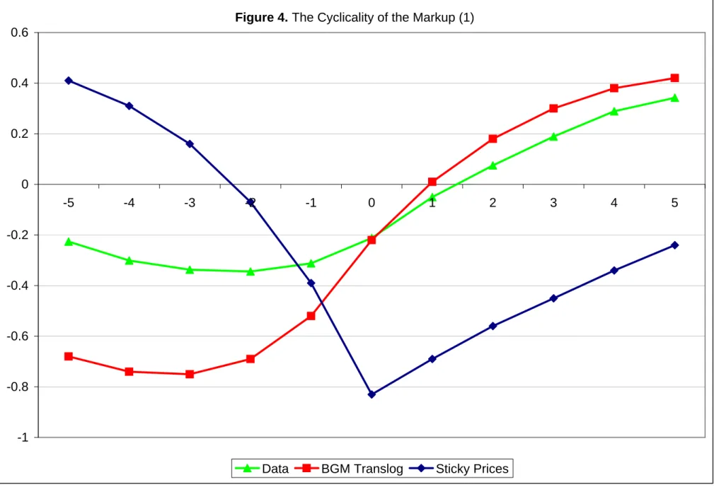
Numerical examples show that the responses to aggregate productivity and deregulation shocks under simple, but plausible specifications of interest rate setting are close to the flexible-price responses. Exogenous interest rate cuts induce the economy to expand, but reduce entry because the associated increase in real wages increases the cost of firm creation and the expected return from investing in new products falls. With productivity shocks as the source of fluctuations and an empirically plausible, simple rule for interest rate setting involving interest rate smoothing and a response to expected producer price inflation, the cyclical properties of endogenous variables are very close to those of the flexible-price counterpart and, in turn, to those of the benchmark RBC model, as documented by BGM. In contrast to the flexible-price model with translog preferences studied in BGM, sticky prices with C.E.S. preferences yield too much markup countercyclicality and a counterfactual time profile of this cyclicality. This happens because the markup is no longer tied to the number of producers as in BGM with translog preferences. On the bright side, aggregate profits remain procyclical (consistent with stylized facts) even in the presence of a very countercyclical markup, and the model remains able to explain the procyclicality of business creation.

1 2

Sbordone (2002) showed that using this corrected measure does not affect the estimates obtained when using the baseline markup proxy. Our framework suggests a specific calibration scheme for the share of overhead labor used in this correction, based on the share of labor used for creating new products.

Producer entry and product creation pose an interesting question for the modeling of nominal rigidity. When a new entrant makes itsfirst price setting decision, we must take a stand on whether it operates as all pre-existing producers do, subject to the same nominal rigidity — thus preserving the symmetry across producers that is a feature of the Rotemberg (1982) model —, or whether it sets its price in flexible fashion, but knowing that it will face a cost of adjusting its price in all subsequent periods. We begin our analysis by assuming that new entrants inherit the same price rigidity as pre-existing firms. This considerably simplifies the model and allows us to obtain an initial set of analytical and numerical results. We then turn to the model in which new entrants set prices inflexible fashion, but knowing that they will be subject to a cost of price adjustment from the following period on.13 In this case, nominal rigidity results in heterogeneity in price levels across cohorts of producers that entered the economy at different points in time, and the aggregate degree of nominal rigidity is endogenous: Expansions are associated with lower aggregate rigidity because the number of new entrants whose decision is not influenced by past price setting increases. We show that the log-linear version of this extended model can still be solved in tractable fashion, and we explore the consequences of endogeneity in aggregate rigidity by means of numerical examples. Plausible parameter values imply responses to shocks that are virtually indistinguishable from those of the benchmark model. Since we assume that average product turnover is realistically small at quarterly frequency, small changes in the fraction of firms that set prices in more flexible fashion triggered by shocks have negligible aggregate consequences, and the benchmark model in which new entrants inherit the same price adjustment cost as incumbents yields robust conclusions.

As in BGM, we explore the consequences of non-C.E.S. preferences by replacing the familiar Dixit-Stiglitz (1977) variety aggregator with a general, homothetic specification of symmetric pref-erences — parametrized in translog form for model solution purposes. This implies that the elasticity of substitution across products increases with the number of producers, introducing an additional effect of the number of available goods on inflation in the New Keynesian Phillips curve. In our numerical examples, this extension yields conclusions that are similar to those of the benchmark model, although it further improves the performance of the model on the inflation persistence front. Lewis (2006) and Elkhoury and Mancini Griffoli (2006) develop models with nominal rigidity that are closest to the one studied here. Lewis introduces monopoly power in the labor market and sticky wages in familiar Calvo (1983)-Yun (1996) fashion into the BGM model. She documents

1 3_{For completeness of comparison, we also consider a version of the model in which new price setters simply set}

VAR evidence that monetary policy expansions result in increasedfirm entry by boosting aggregate demand, and she shows that the sticky-wage model reproduces this evidence. Elkhoury and Mancini Griffoli assume that entry costs in the BGM model take the form of fees paid to lawyers with monopoly power. Under nominal rigidity, the lawyers set the entry fees in Calvo-Yun fashion and, as in Lewis, a monetary expansion that boosts the economy results in increased firm entry. Monetary policy expansions boost firm entry in these models because they induce the real cost of product creation to fall.14 Bergin and Corsetti (2005) document VAR evidence on the consequences of exogenous changes in monetary policy for entry similar to that in Lewis’ paper. They set up a model with entry and one-period price rigidity that replicates this evidence, and they characterize optimal monetary policy and the properties of shock transmission. In Bergin and Corsetti’s model, monetary expansions induce increasedfirm entry by increasing discounted expected future profits. We show that a version of our model in which entry requires purchases of materials rather than hiring labor generates increased entry in response to monetary policy shocks by removing the tight connection between marginal production cost and the value of thefirm embedded in the benchmark setup. Berentsen and Waller (2007) contribute to this literature on monetary policy withfirm entry by introducing endogenous seller entry subject to an entry fee in Lagos and Wright’s (2005) model, in which informational frictions motivate the existence of money as a medium of exchange. Price posting in advance of entry constitutes a price rigidity similar to Bergin and Corsetti’s in their model. They show that the Friedman rule (zero nominal interest rate) is optimal in their model withfixed entry costs. But departures from the Friedman rule are optimal when congestion effects cause entry costs to increase with the number offirms.

The rest of the paper is organized as follows. Section 2 presents our benchmark model. Section 3 obtains the results on optimal monetary policy in the benchmark setup. Section 4 discusses the implications of endogenous entry and product variety for the New Keynesian Phillips curve. Section 5 studies monetary policy through interest rate setting in our model. Section 6 illustrates the business cycle properties of the model. Section 7 discusses the main results of the extensions we explore: the assumption that entry requires materials rather than labor, the alternative assumptions on initial price setting by new entrants, and non-C.E.S. preferences. Section 8 concludes.

1 4

The models in Lewis (2006) and Elkhoury and Mancini Griffoli (2006) are in principle subject to one of the problems that our approach aims to address: They rely on monopoly power as a stepping stone for nominal rigidity, but they abstract from entry (by workers or lawyers) in the presence of monopoly profits.

2

The Model

Household Preferences and the Intratemporal Consumption Choice

We consider a cashless economy as in Woodford (2003). The economy is populated by a unit mass of atomistic, identical households. The representative household supplies Lt hours of work

in each period t in a competitive labor market for the nominal wage rate Wt and maximizes

expected intertemporal utility Et£P∞s=tβs−tU(Cs, Ls)

¤

, where Ct is consumption and β ∈ (0,1)

the subjective discount factor. The period utility function takes the form U(Ct, Lt) = lnCt−

χ(Lt)1+1/ϕ/(1 + 1/ϕ), χ >0, where ϕ≥ 0 is the Frisch elasticity of labor supply to wages, and

the intertemporal elasticity of substitution in labor supply.

At timet, the household consumes the basket of goodsCt, defined over a continuum of goodsΩ:

Ct =

³R

ω∈Ωct(ω)

θ−1/θ_dω´θ/(θ−1)_{, where θ > 1 is the symmetric elasticity of substitution across}

goods. At any given time t, only a subset of goods Ωt ⊂ Ω is available. Let pt(ω) denote the

nominal price of a good ω _∈ Ωt. The consumption-based price index for the home economy is

then Pt =³R_ω∈Ωtpt(ω)1−θdω

´1/(1−θ)

, and the household’s demand for each individual goodω is ct(ω) = (pt(ω)/Pt)−θCt.

Firms

There is a continuum of monopolistically competitive firms, each producing a different variety ω _∈ Ω. Production requires only one factor, labor. Aggregate labor productivity is indexed by Zt, which represents the effectiveness of one unit of labor. Productivity is exogenous and follows

an AR(1) process in percent deviation from its steady-state level. Output supplied by firm ω is yt(ω) =Ztlt(ω), wherelt(ω)is the firm’s labor demand for productive purposes. The unit cost of

production, in units of the consumption good Ct, iswt/Zt, where wt≡Wt/Pt is the real wage.

Prior to entry, firms face a sunk entry cost of fE,t effective labor units, equal to wtfE,t/Zt

units of the consumption good. There are no fixed production costs. Hence, all firms that enter the economy produce in every period, until they are hit with a “death” shock, which occurs with probability δ _∈(0,1)in every period. We assume that the entry cost fE,t is exogenous and treat

changes in fE,t as changes in market regulation.

Firms face nominal rigidity in the form of a quadratic cost of adjusting prices over time (Rotem-berg, 1982). Specifically, the real cost (in units of the composite basket) of output-price inflation

volatility around a steady-state level of inflation equal to0 facing firmω is: pact(ω)≡ κ 2 µ pt(ω) pt−1(ω) − 1 ¶2 pt(ω) Pt y_tD(ω), κ_≥0.

This expression is interpreted as the amount of marketing materials that the firm must purchase when implementing a price change. We assume that this basket has the same composition as the consumption basket. The cost of adjusting prices is proportional to the real revenue from output sales,(pt(ω)/Pt)yDt (ω), where yDt (ω)is firmω’s output demand.

Firms face demand for their output from consumers and firms themselves when they change prices. In each period, there is a mass Nt of firms producing and setting prices in the economy.

When a newfirm sets the price of its output for thefirst time, we appeal to symmetry acrossfirms and interpret the t₋1 price in the expression of the price adjustment cost for that firm as the notional price that the firm would have set at time t₋1 if it had been producing in that period. An intuition for this simplifying assumption is that allfirms (even those that are setting the price for the first time) must buy the bundle of goods pact(ω) when implementing a price decision.15

It should be noted, however, that this assumption is entirely consistent both with the original Rotemberg (1982) setup and with our timing assumption below. Specifically, new entrants behave as the (constant number of) price-setters do in Rotemberg’s framework, where an initial condition for the individual price is dictated by nature. In our framework, new entrants at any time t who start producing and setting prices at t+ 1 are subject to precisely the same assumption as price setters in Rotemberg’s original setup. Moreover, the assumption that a new entrant, at the time of itsfirst price setting decision, knows the average product price last period is consistent with the timing assumption that an entrant starts producing only one period after entry, hence being able to ‘learn’ the average product price during the entry period.16

The total demand for the output offirm ω is thus

yD_t (ω)_≡ µ pt(ω) Pt ¶−θ (Ct+P ACt),

where P ACt ≡Ntpact(ω), and we used symmetry acrossfirms in the definition of the aggregate

demand of the consumption basket for price adjustment purposes P ACt.

Let ρt(ω) ≡ pt(ω)/Pt denote the real price of firm ω’s output. Then, firm ω’s real profit in

1 5

We relax this assumption below.

1 6_{Symmetry of the equilibrium will implypt}

periodt(distributed to households as dividend) can be written as dt(ω) =ρt(ω)ytD(ω)−wtlt(ω)− κ 2 µ pt(ω) pt−1(ω) − 1 ¶2 ρt(ω)yDt (ω).

The real value of thefirm at timet(in units of consumption) is the expected present discounted value of future profits fromt+ 1on, discounted with the household’s stochastic discount factor (see below): vt(ω) =Et ∞ X s=t+1 Λt,sds(ω), (1)

where Λt,s ≡[β(1−δ)]s−tUC(Cs, Ls)/UC(Ct, Lt) is the discount factor applied by households to

future profits fromfirm ω (which faces a probability δ of being hit with the “death” shock in each period).

At timet,firmω chooseslt(ω)andpt(ω)to maximizedt(ω) +vt(ω)subject toyt(ω) =ytD(ω),

taking wt, Pt, Ct, P ACt, and Zt as given. Letting λt(ω) denote the Lagrange multiplier on the

constraintyt(ω) =ytD(ω), thefirst-order condition with respect to lt(ω)yields:

λt(ω) =

wt

Zt

.

The shadow value of an extra unit of output is simply thefirm’s marginal cost, common across all firms in the economy.

The first-order condition with respect to pt(ω) yields:

pt(ω) =μt(ω)Ptλt(ω).

Firmω sets the price as a markup (μt(ω)) over nominal marginal cost, where the markupμt(ω)is

given by μt(ω)≡ θyt(ω) (θ₋1)yt(ω) ∙ 1₋κ₂³ pt(ω) pt−1(ω)−1 ´2¸ +κΥt , Υt≡yt(ω) pt(ω) pt−1(ω) µ pt(ω) pt−1(ω)− 1 ¶ −Et " Λt,t+1yt+1(ω) Pt Pt+1 µ pt+1(ω) pt(ω) ¶2µ pt+1(ω) pt(ω) − 1 ¶# .

As expected, the markup reduces to θ/(θ₋1) in the absence of nominal rigidity (κ= 0) or if the pricept(ω) is constant.

Firm Entry and Exit

In every period, there is an unbounded mass of prospective entrants. These entrants are forward looking, and correctly anticipate their future expected profits dt(ω) in every period as well as the

probability δ (in every period) of incurring the exit-inducing shock. We assume that entrants at time t only start producing at time t+ 1, which introduces a one-period time-to-build lag in the model. The exogenous exit shock occurs at the very end of the time period (after production and entry). A proportionδof new entrants will therefore never produce. Prospective entrants in period tcompute their expected post-entry value given by the present discounted value of their expected stream of profitsvt(ω). This also represents the average value of incumbentfirmsafter production

has occurred (since both new entrants and incumbents then face the same probability1₋δof survival and production in the subsequent period). Entry occurs untilfirm value is equalized with the entry cost, leading to the free entry condition vt(ω) = wtfE,t/Zt. This condition holds so long as the

massNE,t of entrants is positive. We assume that macroeconomic shocks are small enough for this

condition to hold in every period.17 Finally, the timing of entry and production we have assumed implies that the number of producingfirms during periodtis given byNt= (1−δ) (Nt−1+NE,t−1).

Symmetric Firm Equilibrium

In equilibrium, all firms make identical choices. Hence, λt(ω) = λt, pt(ω) = pt, μt(ω) = μt,

ρt(ω) = ρt, lt(ω) = lt, yt(ω) = yt, pact(ω) = pact, dt(ω) = dt, and vt(ω) = vt. The aggregate

output of the consumption basket (used for consumption and to pay price adjustment costs) is

Y_tC _≡Ct+P ACt=Ntρtyt=NtρtZtlt.

The expression of the price indexPtimplies that the relative priceρt and the number of producing

firmsNt are tied by the “variety effect” equationρt=pt/Pt= (Nt) 1

θ−1_.

Let πt denote inflation in producer prices: πt≡pt/pt−1−1. Then, we can write:

μt= θ (θ₋1) h 1₋κ₂(πt)2 i +κ n (1 +πt)πt−β(1−δ)Et h Ct Ct+1 Nt Nt+1 YC t+1 YC t (1 +πt+1)πt+1 io.

This can be simplified further by noting thatP ACt=κ(πt)2YtC/2, so thatCt=

h

1₋κ(πt)2/2

i Y_tC,

to obtain: μt= θ (θ₋1)h1₋κ₂(πt)2 i +κ ½ (1 +πt)πt−β(1−δ)Et ∙ 1−κ2(πt) 2 1−κ2(πt+1) 2 Nt Nt+1(1 +πt+1)πt+1 ¸¾. (2)

Log-linearization of this equation delivers our model’s New Keynesian Phillips curve incorporating the effect of endogenous product variety, which we discuss in detail in Section 4.

Household Budget Constraint, Saving, and Labor Supply

Households hold two types of assets: shares in a mutual fund of firms and bonds. Let xt be the

share in the mutual fund of firms held by the representative household entering period t. The mutual fund pays a total profit in each period (in units of currency) that is equal to the total profit of allfirms that produce in that period,PtNtdt. During periodt, the representative household buys

xt+1 shares in a mutual fund ofNH,t≡Nt+NE,t firms (those already operating at timet and the

new entrants). OnlyNt+1 = (1−δ)NH,t firms will produce and pay dividends at timet+ 1. Since

the household does not know whichfirms will be hit by the exogenous exit shockδ at thevery end

of periodt, itfinances the continuing operation of all pre-existingfirms and all new entrants during periodt. The date t price of a claim to the future profit stream of the mutual fund of NH,t firms

is equal to the average nominal price of claims to future profits of home firms,Vt≡Ptvt.

The household enters period t with nominal bond holdings BN,t and mutual fund share

hold-ings xt. It receives gross interest income on bond holdings, dividend income on mutual fund share

holdings and the value of selling its initial share position, and labor income. The household al-locates these resources between purchases of bonds and shares to be carried into next period and consumption. The period budget constraint (in units of currency) is:

BN,t+1+VtNH,txt+1+PtCt= (1 +it−1)BN,t+ (Dt+Vt)Ntxt+

¡

1 +τ_tL¢WtLt+TtL,

whereit−1 denotes the nominal interest rate on holdings of bonds betweent−1 andt,Dtdenotes

nominal dividends (Dt ≡ Ptdt), τtL is a labor subsidy whose role we discuss below, and TtL is a

lump-sum tax satisfying the constraint T_tL=₋τ_tLWtLt in equilibrium. Dividing both sides byPt

and denoting holdings of bonds in units of consumption with Bt+1≡BN,t+1/Pt, we can write

Bt+1+vtNH,txt+1+Ct= (1 +rt)Bt+ (dt+vt)Ntxt+

¡

where1+rt is the gross, consumption-based, real interest rate on holdings of bonds betweent−1

and t, defined by 1 +rt ≡ (1 +it−1)/

¡

1 +πC_t ¢, with πC_{t ≡} Pt/Pt−1−1, and tLt ≡ TtL/Pt. The

home household maximizes its expected intertemporal utility subject to this budget constraint. The Euler equations for bond and share holdings are:

(Ct)−1 =βEt " 1 +it 1 +πC t+1 (Ct+1)−1 # and vt=β(1−δ)Et "µ Ct+1 Ct ¶−1 (vt+1+dt+1) # .

As expected, forward iteration of the equation for share holdings and absence of speculative bubbles yield the asset price solution in equation (1).18

Thefirst-order condition for the optimal choice of labor effort requires that the marginal disutil-ity of labor be equal to the marginal utildisutil-ity from consuming the real wage received for an additional unit of labor: χ(Lt) 1 ϕ ₌¡_{1 +τ}L t ¢wt Ct .

Aggregate Accounting and Equilibrium

Aggregating the budget constraint (3) across households and imposing the equilibrium conditions Bt+1 =Bt= 0 andxt+1 =xt= 1,∀t, yields the aggregate accounting identity Yt≡Ct+NE,tvt=

wtLt+Ntdt, where we defined GDP, Yt: Consumption plus investment (in new firms) must be

equal to income (labor income plus dividend income).

Labor market equilibrium requires Ntlt+NE,tfE,t/Zt = Lt: The total amount of labor used

in production and to set up the new entrants’ plants must equal aggregate labor supply. (Of course, this condition is redundant once equilibrium in goods and asset markets is imposed.) The equilibrium conditions of our benchmark model are summarized in Table 1.

Table 1. Benchmark Model, Summary Pricing ρt=μtw_Zt_t Markup μt= θ (θ−1)[1−κ2(πt) 2_]+κ (1+πt)πt−β(1−δ)Et Ct Ct+1 Nt Nt+1 Y C t+1 Y C_t (1+πt+1)πt+1 Variety effect ρt= (Nt) 1 θ−1 Profits dt= ³ 1_−μ1 t − κ 2(πt) 2´YC t Nt Free entry vt=wtf_ZE,t_t

Number of firms Nt= (1−δ) (Nt−1+NE,t−1) Intratemporal optimality χ(Lt) 1 ϕ ₌¡_{1 +τ}L t ¢_wt Ct

Euler equation (shares) vt=β(1−δ)Et

∙_³ Ct+1 Ct ´−1 (vt+1+dt+1) ¸ Euler equation (bonds) (Ct)−1 =βEt

h 1+it 1+πC t+1 (Ct+1)−1 i Output of consumption sector Y_tC =h1₋κ₂ (πt)2

i−1

Ct

Aggregate accounting Ct+NE,tvt=wtLt+Ntdt

CPI inflation 1+πt

1+πC t

= ρt

ρt−1

The model is closed by specifying a rule for nominal interest rate setting by the monetary authority, the setting of the labor subsidy τ_tL, and processes for the exogenous entry costfE,t and

productivity Zt.

3

Price Stability with Endogenous Entry and Product Variety

Theflexible-price analysis of BGM leaves inflation in consumer and producer prices — respectively, Ptand pt — indeterminate because monetary policy has no real effect in the flexible-price, cashless

economy, and we need not concern ourselves with the paths of nominal variables in order to solve for real ones. When prices are sticky, this is no longer the case. Specifically, given a change in the number of producersNtand the associated movement in the relative priceρtimplied by the variety

effect equation ρt =pt/Pt = (Nt) 1

θ−1_{, the allocation of this relative price movement to changes in}

producer or consumer prices is important for the dynamics of real variables and welfare. In turn, producer price inflation is a determinant offirm entry — and thusNt— via its impact onfirm profits.

This section studies optimal monetary policy in our model and the optimal allocation of variety effects to producer versus consumer prices.

Our analysis of optimal monetary policy builds on results in Bilbiie, Ghironi, and Melitz (2006). We show there that the flexible-price version of the economy described above is efficient — the competitive equilibrium coincides with the social planner’s optimum — if labor supply is inelastic (ϕ = 0) and Lt = 1 ∀t. The reason is that, with C.E.S. Dixit-Stiglitz preferences, the profit

destruction externality generated by producer entry (which reduces demand for each individual firm) is exactly matched by the consumer’s love for variety — both determined by the elasticity of substitution θ. The flexible-price economy is inefficient if ϕ > 0 because there is a misalignment of markups across the items the consumer cares about (consumption, priced at a markup over marginal cost, and leisure, priced competitively), but efficiency is restored if the labor subsidy τ_tL is equal to the net markup of pricing over marginal cost, 1/(θ₋1) in all periods. This subsidy aligns markups across consumption goods and leisure while preserving the expected profitability of firm entry, thus inducing the efficient equilibrium. We assume thatτ_tL= 1/(θ₋1)_∀tbelow.

Sticky prices imply a time-varying markup whenever producer prices are changing over time. As shown in Bilbiie, Ghironi, and Melitz (2006), markup non-synchronization across periods (as well as across states and arguments of the utility function) generates inefficiency compared to the planner’s optimum. Since in this particular model time variation of the markup in the competitive equilibrium is due to producer price inflation, we expect a zero rate of inflation in producer prices to be the optimal monetary policy chosen by a planner. The following proposition confirms that this is indeed the case. To isolate our main result, we prove the proposition for the case of inelastic labor and then briefly discuss the elastic labor case. As in Bilbiie, Ghironi, and Melitz (2006), we assume that the planner chooses the amount of labor that is allocated to producing existing varieties, which, in turn, determines the number of produced varieties. In addition, in this paper, the planner also chooses the rate of producer price inflation.

Proposition 1 The optimal rate of producer price inflation πt chosen by a social planner is zero.

The proof of Proposition 1 is in an Appendix available on request. The intuition is straightfor-ward: Producer price inflation acts as a tax on firm profits in our model, as can be seen directly in the corresponding equation in Table 1 (inflation erodes the share of total profits in consump-tion output both directly and by its impact on markups). It distorts firm entry decisions and the allocation of labor to creation of new firms versus production of existing goods, resulting in sub-optimal consumption and lower welfare. Optimal policy, therefore, aims to stabilize producer price inflation at zero. Importantly, however, while producer prices must be stabilized, the optimal rate

of consumer price inflation must move freely to accommodate changes in the number of varieties: 1 +π_tC∗ = µ ρ∗_t ρ∗ t−1 ¶−1 = µ N_t∗ N∗ t−1 ¶−θ−11 ,

where a star denotes variables in the efficient equilibrium. Given the evidence of bias in the measurement of CPI inflation (precisely due to poor accounting for new varieties) convincingly documented by Broda and Weinstein (2006), we view this normative implication of our model as “good news.” The central bank should target inflation in producer prices rather than (mismeasured) CPI inflation.

When labor supply is elastic, the subsidyτL

t = 1/(θ−1)ensures that the flexible-price

equilib-rium is efficient, removing the wedge otherwise present between the marginal rates of substitution and transformation between consumption and leisure. In this case, price stickiness distorts both the total amount of labor supplied and its allocation to creation of new firms and production of existing goods. It is easy to verify that a zero rate of inflation in producer prices is still the optimal monetary policy.

The optimality of producer price stability with inelastic labor supply highlights a new argument for price stability (at the producer level) implied by endogenous entry and product variety. In a model with exogenously fixed number of firms and inelastic labor supply, time variation in the markup would have no impact on the equilibrium path of consumption and welfare: Consumption would be simply determined by the exogenous productivity and labor supply regardless of markup dynamics. Endogenous entry and product variety imply that markup variation reduces welfare by distorting entry decisions and the allocation of the fixed amount of labor to firm creation versus production of existing goods. This introduces a role for monetary policy in welfare maximization by stabilizing producer price inflation at zero — and the markup at itsflexible-price level. We discuss implementation of the optimal monetary policy by setting the nominal interest rate below.

4

The New Keynesian Phillips Curve and the Log-Linear Model

This section describes the implications of endogenous entry and product variety for the New Key-nesian Phillips curve and presents the key log-linear equations of the model.

The New Keynesian Phillips Curve

To study the propagation of shocks and compute second moments of the endogenous variables implied by assumptions on the processes for exogenous shocks, we log-linearize the model around the efficient steady state with zero inflation under assumptions of log-normality and homoskedasticity. We denote percent deviations from steady state with sans serif fonts. Our model’s version of the New Keynesian Phillips curve follows from log-linearizing equation (2):

πt=β(1−δ)Etπt+1−

θ₋1

κ μt, (4)

where πt and μt now denote percent deviations from steady state (of gross inflation in the case of

πt).

Since ρt = pt/Pt = (Nt) 1

θ−1 _{and optimal firm pricing implies μ}

t =ρt/λt =ρtZt/wt, it follows

thatμt= (Nt) 1

θ−1_{Zt/wt, or, in log-linear terms:}

μt=

1

θ₋1Nt−(wt−Zt). (5)

(With a constant number of firms, this relation reduces to the familiar negative relation between markup and marginal cost of the benchmark New Keynesian model.) Substituting (5) into (4) yields: πt=β(1−δ)Etπt+1+ θ₋1 κ (wt−Zt)− 1 κNt. (6)

Equation (6) is a New Keynesian Phillips curve relation that ties firm-level inflation dynamics to marginal cost in a standard fashion. Importantly, the effect of marginal cost is adjusted to reflect the number of producers that operate in the economy. This is a predetermined, state variable, which introduces directly a degree of endogenous persistence in the dynamics of product price inflation in the Phillips curve.

Furthermore, our model links the dynamics of inflation to asset prices in an endogenous way, as can be seen by combining (6) with the log-linear free entry condition to obtain:

πt=β(1−δ)Etπt+1+

θ₋1

κ (vt−fE,t)−

1

κNt. (7)

This equation ties inflation dynamics to the relative price of investment in new firms. It stipulates that, for given expected inflation and number offirms, inflation is positively related to equity prices.

Together with the no-arbitrage condition between bonds and equity implied by optimal household behavior, this connection between inflation and equity prices (and thus capital accumulation in our model) plays a crucial role for the determinacy and stability properties of interest rate setting that we discuss below.

Finally, using the definition of CPI inflation, we can write the New Keynesian Phillips curve for consumption-based inflation:

πC_t =β(1₋δ)EtπCt+1+ θ₋1 κ (wt−Zt)− 1 κNt− 1 θ₋1[Nt−Nt−1−β(1−δ) (Nt+1−Nt)], (8)

whereπC_t now denotes the percent deviation of the gross CPI inflation rate from the steady state. Consumption-based inflation displays an additional degree of endogenous persistence relative to firm-level inflation in that it depends directly on the number of firms that produced at time t₋1, which was determined in period t₋2.

Implications for Empirical Exercises

Existing empirical studies estimating the New Keynesian Phillips curve (4), such as Sbordone (2002) and Galí and Gertler (1999), proxy the (unobservable) markup variable with the inverse of the labor share. This is an approximation that holds exactly in a model without endogenous variety. In our model with endogenous variety, however, this relationship no longer holds. Indeed, if one believes product variety to be important for business cycles, the proxy for the markup that one should use is the inverse of the share of labor (in consumption output) beyond the ‘overhead’ quantity (from an aggregate perspective) used to set up new product lines,μt=YtC/[wt(Lt−LE,t)].This

markup measure corresponds closely to the labor share measure used by Rotemberg and Woodford (1999) that takes into account overhead labor. Log-linearization of this equation, when replaced into (4), delivers a relation that is testable empirically.19 Alternatively, exploiting the equation for profits, one could use the inverse of (one minus) the profit share, μt =

¡

1₋DG_t /Y_tC¢−1, as a proxy for markups, whereDG_{t ≡}dtNt+₂κ(πt)2YtC are profits gross of the costs of price adjustment.

Note that since these costs are zero when log-linearizing around a zero-inflation steady-state (and hence consumption is equal to consumption output and gross profits are equal to net profits), the

1 9_{Sbordone (2002) indeed showed that using this corrected measure does not affect the estimates obtained when}

using the baseline markup proxy. Our framework suggests a specific calibration scheme for the share of overhead labor used in this correction, namely: LE/L=δ(μ₋1)/(r+δμ), where we denote steady-state levels of variables by dropping the subscriptt. Under our baseline parametrization below, this is approximately0.20; the upper bound suggested by the empirical results of Basu and Kimball (1997) is0.25.

empirically usable equation will feature only observable variables, i.e., consumption and total profit receipts (or dividends).20

A further implication of our framework for empirical exercises comes from the natural distinc-tion between consumer and producer price inflation in our model: Our framework implies that, in order to overcome measurement issues inherent in using CPI inflation, empirical studies of the Phillips curve should concentrate on producer price inflation (which is also the relevant objective for monetary policy). Construction of CPI data by statistical agencies does not adjust for availabil-ity of new varieties in the specific functional form dictated by the welfare-consistent price index. Furthermore, adjustment for variety, when it happens, certainly does not happen at the frequency represented by periods in our model. Actual CPI data are closer topt(the average price level in our

economy) thanPt. For this reason, when investigating the properties of the model in relation to the

data (for instance, when computing second moments below or in the specification of policy rules that allow for reaction to measured real quantities), one should focus on real variables deflated by a data-consistent price index. For any variable Xt in units of the consumption basket, such

data-consistent counterpart is obtained as XR,t≡PtXt/pt=Xt/ρt.21

Related to this measurement issue, our framework implies an ‘endogeneity bias’ in cost-push shocks in much empirical literature on the New Keynesian Phillips curve. An endogenous term that depends on Nt (due the measurement bias from not accounting for variety) is attributed to

exogenous cost-push shocks when estimating the Phillips curve equation (6) using a proxy for marginal cost without variety.

When the variety effect is removed from the welfare-consistent equity price, the Phillips curve (7) becomes:

πt=β(1−δ)Etπt+1+

θ₋1

κ (vR,t−fE,t), (9) where vR,t is the value of thefirm/price of shares net of the variety effect. For given expectations

of future inflation, actual inflation is increasing in the data-consistent price of equity.

2 0

We leave estimation of Phillips curves using these alternative profit-based proxies for the markup for future research.

2 1

Returning to the normative prescription that the central bank should stabilize producer prices, our model implies that if the central bank targeted CPI inflation, the bias in its measurement would indeed be beneficial to the extent that biased CPI inflation is closer to producer price inflation than welfare-consistent consumer price inflation.

The Log-Linear Model

The log-linear model can be reduced to the following equations (plus the New Keynesian Phillips curve (4)): Nt+1 = [1 +r+ψ]Nt−(r+δ+ψ) (θ−1)Ct−ψ(θ−1)μt+ ((r+δ+ψ) (θ−1) +δ)Zt−δfE,t, (10) Ct= 1₋δ 1 +rEtCt+1− ∙ 1₋δ 1 +r 1 θ₋1− r+δ 1 +r ¸ Nt+1+ 1 θ₋1Nt (11) + ∙ 1₋δ 1 +r − r+δ 1 +r(θ−1) ¸ μt+1−μt− 1₋δ 1 +rEtfE,t+1+fE,t, EtCt+1 =Ct+it−Etπt+1+ 1 θ₋1Nt+1− 1 θ₋1Nt, (12)

where we definedψ _≡ϕ[(r+δ) (θ₋1) +δ]/(θ₋1), which is zero when labor supply is inelastic. The model is closed by specifying the conduct of monetary policy (via the setting of the nominal interest rateit) over the business cycle, which we discuss below.

5

Monetary Policy over the Business Cycle

In this section, we discuss determinacy and stability properties of simple rules for nominal interest rate setting over the business cycle and the implementation of the optimal policy of producer price stability.

Simple Policy Rules

For illustrative purposes, we consider the following class of simple inflation-targeting rules for interest rate setting:

it=τiit−1+τ Etπt+s+τCEtπCt+s+ξti, 1> τi≥0, τ ≥0, τC ≥0, s= 0,1. (13)

where ξ_ti is an exogenous shock capturing the non-systematic component of monetary policy. We assume that τC = 0when τ > 0 and vice versa, restricting the central bank to reacting to either

producer or consumer price inflation.22 For the reasons we discussed above, a response to welfare-based CPI inflation is suboptimal (and not feasible in reality due to the measurement problems

we mentioned). In considering this scenario, we abstract from normative prescriptions and mea-surement issues; rather, we ask the question: What would the response of the economy to various shocks be if the central bank could monitor movements in welfare-consistent CPI inflation and followed a rule involving the latter?

Determinacy and Stability

In this section, we study the determinacy and stability properties of our model under different monetary policy rules. To analyze local determinacy and stability of the rational expectation equilibrium, we can focus on the perfect foresight, no-fundamental-shock version of the system formed by (4), (10), (11), and the equation obtained by substituting the monetary policy rule (13) into the Euler equation for bonds (12). To begin with, consider the simple rule in which the central bank is responding to expected producer price inflation with no smoothing: it =τ Etπt+1.

The following Proposition establishes that the Taylor Principle holds in our model economy for all plausible combinations of parameter values.

Proposition 2 Let γ_≡[1₋β(1₋δ)]/[β(1₋δ)].Assume that ϕ= 0, and β, δ, and θ are such that 1₋γ(θ₋1)>0, β >1/2, θ >2, andτ <¯τ = (κ+θ₋1)/(θ₋1). Thenτ > 1 is necessary and sufficient for local determinacy and stability.

As for Proposition 1, the proof of Proposition 2 is in the Appendix available on request. We remark that the parameter restrictions in Proposition 2 are sufficient conditions for the Taylor Principle to hold, and they are extremely weak. For instance, the values ofκandθthat we consider below (κ = 77 and θ= 3.8) imply τ¯ = 28.5: The sufficient condition τ <28.5 is satisfied by any realistic parametrization of interest rate setting. Moreover, while we cannot prove it analytically, we verify numerically that determinacy and stability hold for values of τ well above the threshold

¯

τ for the parameter values we consider.

Validity of the Taylor Principle is an important result given the debate on the Taylor Principle in models with physical capital accumulation. Dupor (2001) shows that passive interest rate setting (τ < 1) is necessary and sufficient for local determinacy and stability in a continuous-time model with physical capital. Carlstrom and Fuerst (2005) study the issue in a discrete-time model with capital and conclude that it is essentially impossible to achieve determinacy with forward-looking interest rate setting. Our result shows that the standard Taylor Principle is restored when capital accumulation takes the form of the endogenous creation of new production lines.

Intuition: The Role of Asset Prices in Monetary Policy Transmission

Since the validity of the Taylor principle in our setup is in striking contrast to results of models with traditional physical capital, an intuitive explanation of this difference is in order. Indeed, the mechanism for this result in our model is centered precisely on the role of the endogenous price of equity — the value of the firm — in our New Keynesian model with free entry. As we anticipated, the explanation relies on one hand on the Phillips curve (9) above that relates inflation and asset prices (net of the variety effect) vR,t and on the other hand on the no-arbitrage condition implied

by the Euler equations for bonds and shares. This condition can be written as:

it−Etπt+1=−vR,t+

1₋δ

1 +rEtvR,t+1+

r+δ

1 +rEtdR,t+1. (14)

Focus first on the policy rule studied in Proposition 2, where the relevant inflation objective is expected product price inflation, and consider the following experiment. Suppose that a sunspot shock unrelated to any fundamental hits the economy, and that (without losing generality) it is located in inflationary expectations, so that all other expected values are taken as given. We wish to show that if the policy rule is passive (the Taylor Principle is violated), this sunspot shock will have real effects, whereas if the policy rule is active the sunspot has no effect. When the Taylor Principle is violated, an increase in expected inflation triggers a fall in the real interest rate. From the no-arbitrage condition (14), this implies that the data-consistent price of shares must rise (a fall in the real return on bonds must be matched by a fall in the real return on shares, which, forfixed expected dividend and future price, means an increase in the share price today). But an increase in the share price implies, by (9), that actual inflation today will rise, and hence that the sunspot is self-fulfilling. When the Taylor Principle is satisfied, the opposite holds: The sunspot triggers an increase in the real interest rate, a fall in today’s share price by no-arbitrage, and a fall in today’s inflation by the Phillips curve, making the sunspot vanish.23

The same mechanism can be easily verified to hold for a policy rule responding to contempora-neous producer price inflation, and indeed to (contemporaneous or expected) inflation in consumer prices. Therefore, we omit the formal statements and proofs of the Taylor Principle for those cases to save space.24

2 3_{This argument does not hinge on having removed the variety effect from equity prices and dividends. The same}

argument can be made by using the Phillips curve equation (7) and the no-arbitrage condition in welfare-consistent terms.

A comparison of our results and intuition with those of Carlstrom and Fuerst (2005) allows us to further emphasize the crucial role of the different type of capital at the core of our model. Carlstrom and Fuerst show that indeterminacy occurs in a discrete-time model with physical capital when the central bank responds to expected future inflation because the no-arbitrage condition between bonds and capital contains no variable dated at time t.This happens because the expected return to capital depends only on future variables determining the marginal product of capital at time t+ 1. In turn, this implies that there is a zero root in the system, and indeterminacy.25 Instead, in our model, the expected return on shares depends on the price of shares today (an endogenous variable), hence removing this ‘zero-root’ problem. Indeed, through today’s price of equity, our model provides a novel link between the no-arbitrage condition and the Phillips curve that is absent in models that do not feature endogenous variety and free entry.

Implementing Price Stability with Endogenous Entry and Product Variety

The efficient,flexible-price equilibrium requires the nominal interest rate to be equal to the ‘Wick-sellian’ interest rate (in Woodford’s, 2003, terminology), i.e., the interest ratei∗

t that prevails when

prices are flexible and producer price inflation is zero. In log-linear terms, the Wicksellian interest rate is: i∗_t =EtC∗t+1−C∗t − 1 θ₋1 ¡ N∗_t+1−N∗_t¢=EtC∗t+1−C∗t +πCt+1∗,

where EtC∗t+1 −C∗t is the risk-free, real interest rate of BGM and πCt+1∗ is the optimal consumer

price inflation that accommodates changes in variety betweentand t+ 1(known at timet). Note, however, that commitment to the policy ruleit =i∗t would result in equilibrium indeterminacy, as

in the standard model with a fixed number of producers discussed in Woodford (2003), because nominal interest rate setting would contain no feedback to variables that are endogenous in the sticky-price equilibrium.

A simple interest rate rule that implements the efficient,flexible-price equilibrium is

ˆıt=τ πt+EtYˆR,tC +1−YˆR,tC , τ >1, (15)

whereˆıt≡it−it∗ is the interest rate gap relative to the Wicksellian interest rate, andYˆR,tC =CˆR,t≡

Ct−[1/(θ−1)]Nt−{C∗t −[1/(θ−1)]N∗t}=CR,t−C∗R,tis the gap between measured consumption

2 5

The problem is only partially solved by the introduction of capital adjustment costs (introduced in order to endogenize the price of capital). Carlstrom and Fuerst show that the Taylor Principle is restored for forward-looking rules only for empirically implausible parametrizations of the adjustment cost.

output and its flexible-price level. The interest rate rule (15) requires the monetary authority to track changes in the Wicksellian interest rate and in expected growth of the consumption output gap, and to respond more than proportionally to inflation. It is possible to verify that the following equation holds for the dynamics of the consumption output gap:

EtYˆR,tC +1−YˆR,tC =ˆıt−Etπt+1.

Substituting the interest rate rule (15) into this equation yields τ πt = Etπt+1, which has unique

solution πt = 0∀t since the Taylor Principle is satisfied. In turn, zero producer price inflation in

all periods implies YˆC

R,t= 0, and, therefore, it=i∗t ∀t.26

6

Business Cycles: Propagation and Second Moments

In this section, we explore the properties of our benchmark model by means of numerical examples. We compute impulse responses to productivity, deregulation, and monetary policy shocks. Next, we compute second moments of our artificial economy and compare them to second moments in the data and those produced by the baseline BGM model withflexible prices and C.E.S. preferences. As shown in BGM, these moments (which also correspond to those under the optimal monetary policy in the sticky-price economy) are very close to those generated by the standard RBC model.

Calibration

In our baseline calibration, we interpret periods as quarters and set β = 0.99 — a standard choice for quarterly business cycle models. We set the size of the exogenous firm exit shockδ = 0.025to match the U.S. empirical level of10percent job destruction per year.27 We use the value of θfrom Bernard, Eaton, Jensen, and Kortum (2003) and setθ= 3.8, which was calibrated tofit U.S. plant and macro trade data.28 We set initial productivity to Z = 1. The initial steady-state entry cost

2 6

Rule (15) is by no means the only interest rate rule that implements the optimal monetary policy. It is of course possible to design alternative rules that achieve this goal.

2 7

Empirically, job destruction is induced by both firm exit and contraction. In our model, the “death” shock δ

takes place at the product level. In a multi-productfirm, the disappearance of a product generates job destruction withoutfirm exit. Since we abstract from the explicit modeling of multi-productfirms, we include this portion of job destruction inδ. As a higherδimplies less persistent dynamics, our choice ofδis also consistent with not overstating the ability of the model to generate persistence.

2 8

It may be argued that the value ofθresults in a steady-state markup that is too high relative to the evidence. However, it is important to observe that, in models without anyfixed cost,θ/(θ₋1)is a measure of both markup over marginal cost and average cost. In our model with entry costs, free entry ensures thatfirms earn zero profits

net of the entry cost. This means that firms price at average cost (inclusive of the entry cost). Thus, although

fE does not affect any impulse response; we therefore set fE = 1 without loss of generality. We

consider different values for the elasticity of labor supply,ϕ, and we set the weight of the disutility of labor in the period utility function, χ, so that the steady-state level of labor effort is 1 — and steady-state levels of all variables are the same — regardless of ϕ.29 We set the price stickiness parameterκ= 77,the value estimated by Ireland (2001). Although Ireland obtained this estimate using a different model, without entry and endogenous variety, our results are not sensitive to changes in the value of this parameter within a plausible range.

Impulse Responses

Productivity

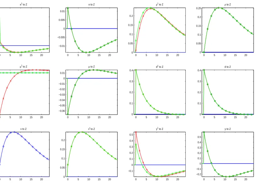
Figure 1 shows the responses (percent deviations from steady state) to a 1 percent increase in productivity for the inelastic labor case. For consistence with the second moment results below, we assume productivity persistence 0.979as in King and Rebelo (1999). The figure compares the efficient flexible-price equilibrium obtained under optimal monetary policy (blue, round markers) with three alternative parametrizations of the monetary policy rule (13). Thefirst is a simple rule responding to expected producer price inflation,it= 1.5Etπt+1 (red, cross markers); the second is

a rule involving interest rate smoothing, it = 0.8it−1+ 0.3Etπt+1 (green, square markers), which

features the same long-run response to expected inflation (1.5) as the previous rule; and the third is a rule responding to expected welfare-consistent CPI inflation,it= 1.5EtπtC+1 (pink, star markers).

Note that the difference between the responses under each of the simple rules and the optimal policy measures the gap relative to theflexible-price equilibrium under the alternative rules. The number of years after the shock is on the horizontal axis, and responses are normalized so that0.3

(for instance) denotes 0.3 percent.

Focus on the responses under the optimal policy. The increase in productivity makes the business environment temporarily more attractive, drawing a higher number of entrants (NE,t),

which translates into a gradual increase in the number of producers (Nt) before entry and the stock

of production lines return to the steady state. The larger number of producers induces marginal cost (wt/Zt — not shown) and the relative price of each product ρt to increase gradually with

unchanged markup. GDP (Yt) and consumption (Ct) increase, and so does investment in newfirms to pricing and average costs. The main qualitative features of the impulse responses below are not affected if we set

θ= 6, resulting in a20percent markup of price over marginal cost as in Rotemberg and Woodford (1992) and several other studies.

2 9

(v_tE _≡vtNE,t) as thefixed labor supply is reallocated toward creation of new products. Interestingly,

firm-level output (yt) is below the steady state during most of the transition, except for an initial

expansion. The effect of a higher relative price prevails on the expansion in consumption demand to push individual firm output below the steady state for much of the transition, with expansion in the number of producers and investment in newfirms responsible for GDP remaining above the steady state throughout the transition. Notably, the dynamics of firm entry result in responses that persist beyond the duration of the exogenous shock, and, for some key variables, display a hump-shaped pattern.30

When comparing responses across policy rules, a remarkable feature of the results is that the dynamics of macroeconomic aggregates under thefirst two simple policy rules are strikingly similar to those in theflexible-price equilibrium. Indeed, the responses of GDP are virtually indistinguish-able, and those of consumption and the number of producers are also very close. Equivalently, the changes in producer price inflation and the markup induced by technology shocks under these pol-icy rules are small. It is worth stressing that this is in contrast with responses in the fixed-variety, benchmark New Keynesian model, where there are quantitatively significant deviations from the flexible-price equilibrium under such simple policy rules. In our model, instead, a simple rule such asit= 1.5Etπt+1, despite not featuring an overly aggressive response to inflation, manages to bring

the economy quite close to its first-best optimum. This is no longer true when monetary policy responds to welfare-consistent CPI inflation: There are more evident differences in the responses of consumption and the number of producers, stemming from the suboptimal response of the cen-tral bank to movements in welfare-based CPI inflation that reflect fluctuations in the number of products.31

Importantly, our model with entry can induce inflation and countercyclical markups, and po-tentially procyclical labor, in response to technology shocks. To understand this result, recall the intuition in the standard New Keynesian model, which implies deflation and procyclical markups in response to productivity increases: Marginal cost falls, prices decrease (there is deflation), but not by as much because of stickiness, so output increases and markups increase too — i.e., the markup is procyclical. In our model with entry, there is an additional channel of shock transmission working in the opposite direction: Positive productivity shocks increase future profits and the value of the

3 0_{The responses of several macroeconomic variables deflated by average prices (the producer price levelpt) rather}

than with the consumption-based price index are qualitatively similar. For instance,CR,t increases, with a hump-shaped response except when policy responds to welfare-based CPI inflation. YR,t also rises, although without a hump.

3 1