I
n recent years, capital restrictions in emerging markets have been substantially reduced. As a result, international financial flows to these countries have risen. Most emerging markets have adopted a pegged exchange rate system in which central banks are committed to keep-ing their domestic currency in terms of the U.S. dollar within narrow bands. Under this system, a country can finance a current account deficit from its reserves or by borrowing from abroad. That is, the country can buy time in handling external deficits without decreasing the monetary base or reducing the public deficit. Such a regime relies on a delicate balance and makes a country vulnerable to shocks in mobile inter-national capital markets, especially with respect to outflows in bank deposits.When international markets are relatively calm, lenders may be willing to finance countries with mildly weak fundamentals. As international conditions deteriorate, however, investors’ perception about a borrower’s creditworthiness may change. Economies that look sound one moment seem riskier the next— not necessarily because of new developments within their borders but perhaps because interconnected countries are in distress. As foreign investors become more risk averse, they may withdraw short-term investments and sell local currency. The country’s central bank must then increase interest rates suffi-ciently to dampen the outflow and avoid a collapse of the pegged exchange rate system. The result of
such reactive strategies may be a credit crunch that spreads from country to country, driving each into economic recessions with high inflation.
In the last decade several developed and devel-oping countries experienced currency crises. For example, the European Monetary System (EMS) was severely undermined by intense speculative pres-sure in 1992–93, which led to the exit of Britain and Italy in 1992. More recently, several emerging market economies underwent large devaluations of their currencies: Mexico in 1994, several Asian countries in 1997, Russia in 1998, and, subsequently, Brazil in 1999, among others. These events cast a bleak out-look for the global financial system and caused widespread economic distress. Even the U.S. econ-omy experienced slowdowns associated with these international events, especially the Mexican and Asian crises.
A “country risk” of currency crisis is not directly observable, but prior currency pressures can be detected in several sectors of the economy. In partic-ular, financial variables reflecting investors’ expecta-tions and banking distress are highly sensitive to changes in the economic environment. This article aims to construct an early warning system for inter-national currency crises using such variables. The system uses a dynamic factor model with regime switching to construct leading indicators of country risk and currency crises. In this model, an unobserv-able factor switches regimes, representing periods
Leading Indicators of Country
Risk and Currency Crises:
The Asian Experience
MARCELLE CHAUVET AND FANG DONG Chauvet is a research economist at the Atlanta Fed. Dong is an assistant professor at Providence College in Rhode Island.
and smooths out noise inherent in monthly data. This smoothing reduces the likelihood of signaling false turning points, which can be a significant problem in the monthly frequency. Second, in contrast to com-posite indicators that are constructed as weighted averages of statistical transformations of their com-ponents, the dynamic factor model takes into account cross-correlations and potential long-term relation-ships among the variables. Finally, the method yields probabilities that can signal turning points in real time. This method contrasts with the rules of thumb used to build some composite indicators, which require the use of substantial ex post data. Because these rules are based on the unusual behavior of some variables compared to their frequency distribution, turning points can be identified and predicted only a couple of months after their occurrence, which undermines their usefulness for real-time forecasting. Thus, the advantage of the proposed approach in comparison with alternative models and rules of thumbs is that it treats foreign exchange market regimes as unobservable priors instead of observed ex post events, and no ad hoc criterion is adopted in determining the crisis state. Instead, the model gen-erates regime probabilities from the leading indica-tors that can be used to signal increases in country risk and potential currency crises in real time.
The approach in this article implements several linear and nonlinear methods to select the variables composing the indicators. For the Asian countries studied, the best candidates are monetary and banking series. The study shows that the leading indicators built from the nonlinear dynamic factor model unveil, both in sample and out of sample, early warning signals of an increase in the country risk and subsequent depreciation of nominal exchange rates experienced by Thailand, Indonesia, and Korea, especially before the 1997 crisis. In gen-eral, phases of the leading index exhibiting a higher mean and volatility precede currency crises, whereas the noncrisis state is associated with a lower mean and volatility.
For all the countries studied, the regime proba-bilities give early signals of the 1997 crisis and reveal a contagion pattern. For Thailand, a crisis was sig-naled six months earlier than the actual one. For Indonesia, the probabilities indicated a crisis seven months before the actual one, which was minimized by preemptive government actions. However, once Thailand’s currency crisis hit, the probability of a cri-sis in Indonesia also increased substantially and thus increased the probability of a crisis in Korea. This finding suggests a contagion pattern that is being further examined in ongoing projects.
of relative calmness and periods prone to currency crises, using a two-state Markov process. The method is applied to evaluate the model’s in-sample and out-of-sample performance in anticipating currency crises in the last two decades in Thailand, Indonesia, and Korea. The dynamic factor index gives early dis-tress signals of country risk and currency crisis, using several financial and banking variables.
Leading indicators have been a successful fore-casting tool adopted by the National Bureau of Economic Research (NBER) since the work of Burns and Mitchell (1946). New econometric models have now been used to explore more formally potential dynamic differences across cycle phases in several
variables. The method used to construct economic indicators is distinct from econometric regression methods. In particular, the goal is not to form a fore-cast of exchange rates based on the information set. Instead, leading indicators are indexes composed of several variables, designed to give early signals of major cyclical changes in exchange rates, particu-larly the beginning and end of cyclical phases (that is, their turning points). Variables that exhibit low power in explaining the linear long-run variance of exchange rates may be highly important in specific situations. In fact, unusually large changes in some variables at particular historical episodes—as opposed to the linear average behavior of the series— can be important independent factors in determin-ing large exchange rate devaluations.
A large theoretical and empirical literature aims to characterize or forecast the recent experiences of currency crises.1Few of these studies, however,
focus on forecasting turning points representing episodes of speculative attacks.
The method this study uses to construct indicators differs from the previous currency crisis literature in several ways. First, since currency crises are caused by different shocks over time, the inclusion of differ-ent variables increases the model’s ability to signal future crises. In addition, the combination of variables reduces measurement errors in the individual series
This article constructs an early warning system
for international currency crises using financial
variables that reflect investors’ expectations
and banking distress.
1. See, for example, the list of more than 100 recent papers and books related to the NBER Project on Exchange Rate Crises in Emerging Market Countries at <www.nber.org/crisis> or the reference list at <www.stern.nyu.edu/globalmacro>.
2. State-owned banks in Indonesia and Korea were regularly allowed to break many prudential regulations without penalty. 3. During the 1984:11–1985:03 period, Thailand abandoned a fixed exchange rate vis-à-vis the dollar. The central bank abolished
general credit restrictions but reimposed restrictions on bank lending rates and lowered the ceiling for loans to priority sectors (see Bekaert and Harvey 1999).
The article first discusses the currency crises experienced by the Asian countries studied. The discussion then presents the data and statistical analysis used to select the leading variables, pre-sents the dynamic factor model used to construct the leading indicators, and reports the in-sample and out-of-sample empirical results.
Currency Crises in Asia
R
adelet and Sachs (1998) study the broad features underlying the recent experiences of currency crises in Asian countries. One striking finding is that typical international and domestic problems were not present before the onset of the crises. In fact, for the most part conditions in international financial mar-kets, commodity marmar-kets, and the trading system were favorable. These countries were not pursu-ing tight anti-inflationary policies, and their real exchange rates were only mildly overvalued because of the persistent inflow of capital. In addition, their overall debt-carrying capacities did not seem to pre-sent imminent risks of default. In particular, Radelet and Sachs find that instability in international lending and self-fulfilling speculative attacks are the most likely explanations for the Asian crisis in 1997. International loan markets may be subject to self-fulfilling crises even when individual creditors act rationally. Changes in investors’ risk perception may result in sharp, costly, and fundamentally unneces-sary panicked reversals in capital flows. In this situa-tion, exchange rates may immediately depreciate under intense pressure. The unwillingness or inabil-ity of the capital market to provide new loans to the illiquid borrowers is a chief factor during crises.Another common feature of these countries prior to the crises was the growing weaknesses in East Asian financial systems resulting from incomplete markets and some market-oriented reforms, which made the countries vulnerable to capital flight. In this regard, the intensity and propagation of the crises were also the result of partial banking and financial reforms that exposed these economies more directly to the instability of international financial markets.
Examples of bank weaknesses were the growth of short-term foreign debt, the rapid expansion of bank credit/lending, the inadequate regulation and supervision of financial institutions, and the sharp
increase in the number of financial institutions and private banks (including foreign and joint venture banks) that could borrow or lend in foreign curren-cies, both on- and offshore.2
These problems made the countries more vul-nerable to a rapid reversal of capital flows that put downward pressure on their currencies. Whereas Radelet and Sachs (1998) find that the problems were centered in the private sector rather than in the government, this article finds that they were also present in the monetary system.
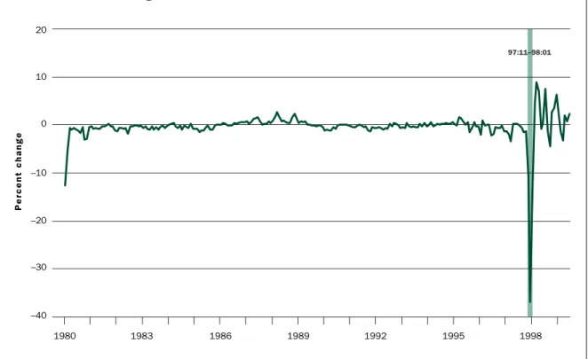
Thailand.Three major currency devaluations in Thailand occurred during the 1981:05–1981:07, 1984:11–1985:03, and 1997:07–1998:01 periods.3
These devaluations of the baht are illustrated in Figure 1, which plots Thailand’s nominal exchange rate in the form of logarithmic first differences (GW_N$BAHT).
During the 1990s, capital inflows into Thailand averaged over 10 percent of gross domestic product (GDP) and reached a remarkable 13 percent of GDP in 1995 alone. These inflows consisted predomi-nantly of borrowing by banks and financial institu-tions. Throughout the decade the government fixed the exchange rate within very narrow bands. In effect, the central bank absorbed the risks of exchange rate movements on behalf of investors and thus encour-aged capital inflows, especially of short-maturity instruments. However, increasing capital inflows put upward pressure on the prices of nontradable goods and services. The real effective exchange rate appre-ciated by more than 25 percent between 1990 and early 1997.
Indonesia.Three major currency devaluations in Indonesia occurred in April 1983, September to
This study demonstrates that the leading
indi-cators of currency crises can be informative
tools for signaling future currency crises in
real time and could thus allow preemptive
counterpolicy measures by the central bank.
Percent change 1980 20 5 15 10 0 –5 –10 1983 1992 –15 1986 1989 1995 1998 –20 81:05–81:07 84:11–85:03 97:07–98:01
Thailand’s Nominal Exchange Rate
Source: Datastream, International Financial Statistics database
Percent change 1980 40 20 0 –20 –40 1983 1992 –60 1986 1989 1995 1998 –80 83:04 86:09–86:10 97:08–98:12 F I G U R E 2
Indonesia's Nominal Exchange Rate
4. For example, although some series are available monthly, their release takes place two to three months later.
5. A variable is said to be (weakly) stationary if the mean and autocovariances of the series do not depend on time. Any series that is not stationary is said to be nonstationary. The augmented Dickey-Fuller (1979) and Phillips-Perron (1988) tests were used to test for stationarity. In addition, Perron’s (1989) test was also used to test for nonstationarity against the alternative of deterministic trend in the presence of sudden changes in the series.
October 1986 (Sachs, Tornell, and Velasco 1996), and August 1997 to December 1998. The devalua-tions of the rupiah are shown in Figure 2, which plots Indonesia’s nominal exchange rate in the form of logarithmic first differences (GW_N$RUPIAH).
Capital inflows to Indonesia in the 1990s aver-aged a more modest 4 percent of GDP and were mostly in the form of borrowing by private corpora-tions. Indonesia’s government fixed the exchange rate subject to small and predictable changes. Here too the government absorbed the borrowing risks undertaken by the private sector, inducing higher inflows of capitals. As a result, the real effective exchange rate appreciated by more than 25 percent between 1990 and early 1997.
Korea.The only major nominal devaluation of the Korean won was related to the Asian crisis, which hit the country in November 1997. Annual capital inflows averaged over 6 percent of GDP between 1990 and 1996. The government maintained the exchange rate with small and predictable changes and absorbed the
loan risks. The real effective exchange rate appreci-ated by 12 percent between 1990 and early 1997. Figure 3 plots the logarithmic first differences of Korea’s nominal exchange rate (GW_N$WON).
Data and Statistical Analysis
S
election of candidate leading variables.In the first triage, the variables were selected accord-ing to several criteria, such as their frequency, sam-ple size, and how quickly new releases of the series were available. For these indicators to be useful for real-time forecasting of currency crises, the variables used should be available at least at the monthly fre-quency and be timely.4We found approximately tenvariables for each country as potential candidates to predict abrupt changes in nominal exchange rates.
Several econometric procedures were then used to select and rank the potential variables. First, all series were transformed to achieve stationarity.5The
variables were then classified according to their cross-correlation with nominal exchange rates and
Percent change 1980 20 10 0 –10 –20 1983 1992 –30 1986 1989 1995 1998 –40 97:11–98:01 F I G U R E 3
Korea's Nominal Exchange Rate
money supply (M1), net foreign assets and private bank foreign liabilities in billions of rupiah, and offi-cial foreign reserves minus gold in millions of U.S. dollars (Figure 5); and (3) for Korea, domestic credit, net foreign assets and private bank credits from monetary authorities in billions of won, and the CPI (Figure 6).
These data were obtained from the International Financial Statistics database from Datastream. The sample available in monthly frequency covers the 1980:01–1999:06 period for Indonesia and Korea and the 1980:02–1999:06 period for Thailand. Nominal exchange rates are measured in U.S. dol-lars per unit of the national currency.
The Dynamic Factor Model with
Markov Regime Switching
T
his analysis uses a dynamic factor model with Markov regime switching to construct the lead-ing indicators of currency crises for Thailand, Indonesia, and Korea.7This model is a combinationof the linear Kalman filter and Hamilton’s (1989) Markov regime switching model and has been widely their ability to Granger-cause exchange rates.6
Granger causality tests select variables that have a linear predictive content for exchange rates, but not necessarily those that perform well in anticipat-ing peaks and troughs in exchange rate changes. Variables that are poor predictors of linear long-run exchange rate variances may be significant in par-ticular situations. Large changes in such variables during specific historical episodes can be important in predicting large exchange rate devaluations. For this reason, we use probability methods to study the nonlinear relationship of each series to deter-mine whether it anticipates peaks and troughs of exchange rate dynamics. In particular, different specifications of two-state first-order Markov switching models were fitted to each candidate leading variable (see Chauvet and Dong 2002).
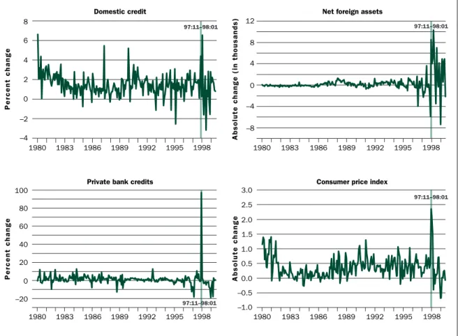
The following leading variables were selected from both linear and nonlinear procedures: (1) for Thailand, domestic credit, net foreign assets and private bank credits from the central bank in bil-lions of baht, and the consumer price index (CPI) (1995 = 100) (see Figure 4); (2) for Indonesia, the
Absolute change
100
–50
–150
Consumer price index Private bank credits
Percent change
8
0
–6
1998
Net foreign assets Domestic credit Absolute change 150 0 Absolute change 3 1 –1 1980 1983 1986 1992 1995 6 4 2 –4 –2 1989 100 50 –150 –50 –100 1998 1980 1983 1986 1989 1992 1995 1998 1980 1983 1986 1989 1992 1995 50 0 –100 1998 1980 1983 1986 1989 1992 1995 2 0 81:05–81:07 84:11–85:03 97:07–98:01 81:05–81:07 84:11–85:03 97:07–98:01 81:05–81:07 84:11–85:03 97:07–98:01 81:05–81:07 84:11–85:03 97:07–98:01
Thailand: Domestic Credit, Net Foreign Assets, Private Bank Credits, and the Consumer Price Index
6. A Granger causality test determines how much of a current time series can be explained by past values of itself and whether adding lagged values of another series can improve the explanation.
7. A Markov process is a simple stochastic process in which the distribution of future states depends only on the present state and not on how the present state was achieved.
applied to business cycle studies (see, for example, Diebold and Rudebusch 1996; Chauvet 1998; Kim and Nelson 1998).
In this framework, the latent factor for each country—the leading indicator—is constructed as the common correlation underlying the country’s leading financial variables. The motivation for this setup is to combine the leading variables and extract their common characteristics, which switch regimes representing foreign exchange market pressures. The mean and variance of the dynamic factor are subject to discrete regime shifts governed by a two-state Markov process. That is, the foreign exchange market can be either under high pressure to devaluate (state or regime 0) or under low spec-ulative pressure (state or regime 1), with the alter-nation between states controlled by the outcome of the Markov process. Since the probabilistic
infer-ence on crises is based on shocks to several leading variables used for each country, the model used here can give more accurate signals of crises (fewer false or missed signals) than univariate autoregres-sive models with Markov regime switching. (See Chauvet and Dong 2002 for further discussions.)
In-Sample Results
M
aximum likelihood estimates. Table 1 reports the maximum likelihood estimates of the Markov-switching dynamic factor model for Thailand, Indonesia, and Korea. For each country, the analysis shows that regime 0 (high speculative pressure) is characterized by a large variance.For Thailand, estimation shows that the net for-eign asset (NFA) variable is the most sensitive to changes in the country’s leading indicator. A one-unit increase in the factor is associated with a
Percent change
100
–20
–100
Foreign reserves Private bank foreign liabilities
Percent change 20 0 –15 1998 M1 Percent change 80 20 Percent change 30 –10 –50 1980 1983 1986 1992 1995 15 10 5 –10 –5 1989 60 40 –40 0 –20 1998 1980 1983 1986 1989 1992 1995 1998 1980 1983 1986 1989 1992 1995 80 20 –60 1998 1980 1983 1986 1989 1992 1995 10 –30
Net foreign assets
60 40 0 –40 –80 20 0 –20 –40 83:04 86:09–86:10 97:08–98:12 83:04 86:09–86:10 97:08–98:12 83:04 86:09–86:10 97:08–98:12 83:04 86:09–86:10 97:08–98:12 F I G U R E 5
Indonesia: M1, Net Foreign Assets, Private Bank Foreign Liabilities, and Foreign Reserves
least sensitive series to the factor, with a factor coefficient of about 0.30 percent. The leading indi-cator for Korea is highly persistent, with an autore-gressive coefficient of 0.92. The volatility of the leading indicator is about 364 times larger in the crisis state than in the noncrisis state.
Table 2 shows that, for all three countries, the leading indicator of currency crisis is negatively correlated with exchange rates. That is, increases in the level of the leading indicator are associated with currency depreciation. The currency crises for all countries are anticipated by the dynamic factor behavior in state 0, that is, for the high-mean and high-volatility regime.
Variables such as NFA, private bank credits from the central bank, and PBFL are the most useful in signaling speculative pressures and currency crises in these three countries. Crises would also be antic-ipated with a smaller lead by internal macroeco-nomic fundamentals such as domestic credits, the money supply, the CPI, or foreign reserves. This find-ing supports evidence that the currency crises across these three countries are likely to have originated in monthly decrease in NFA of about 5 billion baht,
ceteris paribus. On the other hand, the CPI variable is the least sensitive to changes in the leading indi-cator. The leading indicator for Thailand is highly persistent, with an autoregressive coefficient equal to 0.91. In the crisis state, the volatility of the lead-ing indicator is about 256 times larger than in the normal or noncrisis state.
For Indonesia, the private bank foreign liabilities (PBFL) variable is the most sensitive to changes in the country’s leading indicator. A one-unit increase in the factor is associated with a monthly increase in PBFL of 2.72 percent. The reserves variable, with a factor coefficient of 0.47 percent, is not as sensitive as other variables. The leading indicator for Indonesia is somewhat persistent, with an autoregressive coef-ficient of –0.64. In the crisis state, the volatility of the leading indicator is about 31 times greater than in the noncrisis state.
For Korea, the NFA variable is the most sensitive to changes in the factor; a one-unit increase in the factor is associated with a monthly increase in NFA of 212.39 billion won. As in Thailand, CPI is the
Percent change
100
Consumer price index Private bank credits
Percent change
8
0
1998 Domestic credit
Absolute change (in thousands)
12 Absolute change 3.0 1.0 –1.0 1980 1983 1986 1992 1995 6 4 2 –4 –2 1989 8 4 1998 1980 1983 1986 1989 1992 1995 1998 1980 1983 1986 1989 1992 1995 60 1998 1980 1983 1986 1989 1992 1995 2.0 0.0
Net foreign assets
80 2.5 1.5 0.5 –0.5 0 –4 –8 40 20 0 –20 97:11–98:01 97:11–98:01 97:11–98:01 97:11–98:01
Korea: Domestic Credit, Net Foreign Assets, Private Bank Credits, and the Consumer Price Index
Thailand Indonesia Korea αˆ0 –0.0756 αˆ0 4.9982 αˆ0 0.2075 (0.2190) (2.0785) (0.7200) αˆ1 0.1243 αˆ1 1.8668 αˆ1 0.0950 (0.0550) (0.3120) (0.0340) φˆ 1 0.9133 φˆ1 –0.6442 φˆ1 0.9181 (0.0384) (0.1729) (0.0257) σˆ2 υ0 9.0228 σˆ 2 υ0 28.5281 σˆ 2 υ0 5.5735 (3.9717) (10.9832) (3.8378) σˆ2 υ1 0.0352 σˆ2υ1 0.9139 σˆ2υ1 0.0153 (0.0140) (0.6835) (0.0085) Pˆ 00 0.9277 Pˆ00 0.8641 Pˆ00 0.8835 (0.0680) (0.1083) (0.1352) Pˆ 11 0.9933 Pˆ11 0.9810 Pˆ11 0.9903 (0.0069) (0.0188) (0.0069) σˆ2 GW_DC 0.5136 σˆ 2 GW_M1 4.2514 σˆ 2 GW_DC 1.2626 (0.0689) (0.9551) (0.1473) σˆ2 CH_NFA 622.7890 σˆ 2 GW_NFA 91.1092 σˆ 2 CH_NFA 2431783.9236 (59.0376) (8.7597) (226865.0648) σ ˆ2 CH_PB 242.5626 σˆ 2 GW_PBFL 276.6354 σˆ 2 GW_PB 52.4856 (22.6699) (27.8780) (4.9980) σˆ2 CH_CPI 0.1661 σˆ 2 GW_RESV 38.3251 σˆ 2 CH_CPI 0.0797 (0.0166) (3.6027) (0.0093) λˆ GW_DC 1.0000 λˆGW_M1 1.0000 λˆGW_DC 1.0000
(Restricted) (Restricted) (Restricted)
λˆ
CH_NFA –4.9412 λˆGW_NFA 0.7839 λˆCH_NFA 212.3871
(1.1487) (0.3134) (75.3244)
λˆ
CH_PB 2.6914 λˆGW_PBFL 2.7161 λˆGW_PB 1.6953
(0.6788) (0.5460) (0.3660)
λˆ
CH_CPI 0.2096 λˆGW_RESV 0.4683 λˆCH_CPI 0.2951
(0.0191) (0.1793) (0.0205)
Note: The sample period is 1980:01–1999:06. Asymptotic standard errors (computed numerically) appear in parentheses. The factor mean for crisis state is µˆ
0=αˆ0/(1–φˆ1),and for off-crisis state it is ˆµ1=αˆ1/(1–φˆ1). T A B L E 1
Maximum Likelihood Estimates: Dynamic Factor Model with Regime Switching
Thailand Indonesia Korea
N$RUPIAH –0.4762 N$WON –0.7083
N$BAHT –0.6471 N$BAHT –0.3022 N$BAHT –0.4076
GW_DC 0.7845 GW_M1 0.8823 GW_DC 0.4401
CH_NFA –0.6530 GW_NFA 0.2171 CH_NFA 0.0184
CH_PB 0.5089 GW_PBFL 0.4600 GW_PB 0.4148
CH_CPI 0.2304 GW_RESV 0.1911 CH_CPI 0.6318
T A B L E 2
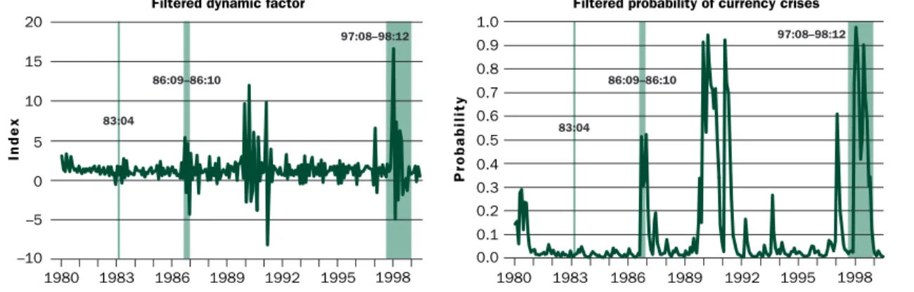
Figure 8 plots the dynamic factor and the proba-bility of currency crises for Indonesia. Both are quite stable, with values close to 0 for most of the sample except around the currency crises. In fact, they display abrupt oscillations in 1986–87, 1989–91, and 1997–98, anticipating the crises. In particular, the factor and probability of currency crises signal the currency crises in 1986:09 and in 1997:08 nine months in advance. On the other hand, the devaluation in 1983:04 was very small. This pattern is also reflected in the probability of currency crises, which indicates weak speculative pressure (around 2 percent in 1982:12). The small probability of currency crises at the end of 1982 reinforces the view that the 1983 devaluation did not originate from strong pressures from the finan-cial sector and was mostly unanticipated. The devaluation in 1986 was much larger in comparison, and the probability of currency crises—ranging from about 11 percent in 1986:06 to 58 percent in 1986:09—gives clear signals of it, indicating stronger speculative pressure. The 1997 devalua-tion was the most severe one experienced by Indonesia (see Figure 2). The probability of cur-rency crises ranged from 19 percent in 1996:11 to 60 percent in 1997:01—seven months prior to the crisis in 1997:08. After the onset of the crisis, the probability, ranging from 15 percent in 1997:10 to almost 100 percent in 1998:01, indicated continu-ous speculative pressure.
One should note that the probability increased substantially between 1989:07 and 1991:04. During this period Indonesia underwent financial liberaliza-tion and experienced fluctualiberaliza-tions in capital inflow (a deceleration in portfolio and other short-term their respective private financial sectors and
mone-tary sectors as a result of unsustainable financial liberalization policies.
For Thailand, in particular, acceleration in the growth rate of domestic credits and increases in the level of private bank credits from the central bank and in the level of the CPI led to increases in the leading indicator of currency crises. Hence, pres-sures to devalue Thailand’s baht are associated with increases in the dynamic factor and with decreases in the level of NFA. For Indonesia, acceleration in the growth rate of money, NFA, PBFL, and reserves are associated with increases in the factor and, therefore, with the devaluation of Indonesia’s rupiah. For Korea, acceleration in the growth rate of domes-tic credits and private bank credits from the central bank and increases in the level of NFA and the CPI are associated with increases in the factor and, hence, with the devaluation of Korea’s won.
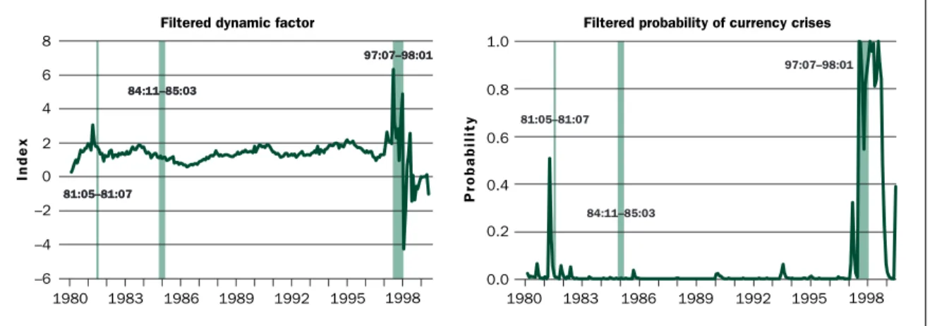
Probabilities of currency crises.Figure 7 plots the dynamic factor (the leading indicator) and the probability of currency crises for Thailand. The lead-ing indicator is quite stable for most of the sample except for the periods prior to the currency crises in 1981:05 and 1997:07, when the factor moves up and down considerably. This pattern can also be observed in the probability of currency crises, which increases substantially in 1981:02 (three months before the 1981:05 currency crisis) and in 1997:01 (six months before the 1997:07 crisis). The factor is less sensitive to the depreciation in 1984:11, when Thailand’s authorities abandoned the fixed exchange rate vis-à-vis the dollar. The economy displayed stronger funda-mentals during this time and was less susceptible to external shocks.
Index
8
0
1998 Filtered dynamic factor
Probability 1.0 1980 1983 1986 1992 1995 6 4 2 –6 –4 1989 0.8 0.6 1998 1980 1983 1986 1989 1992 1995
Filtered probability of currency crises
0.4 0.2 0.0 –2 81:05–81:07 84:11–85:03 97:07–98:01 81:05–81:07 84:11–85:03 97:07–98:01 81:05–81:07 84:11–85:03 97:07–98:01
Thailand: Filtered Dynamic Factor and Filtered Probability of Currency Crises
flows and continued growth in foreign direct invest-ment) while interest rates decreased significantly. However, the exchange rates did not succumb to the high speculative pressure in 1989:07–1991:04 because the government made a preemptive policy response to structural changes in capital inflows (see Radelet and Sachs 1998).
Figure 9 plots the dynamic factor and probability of currency crises for Korea. Again, the dynamic fac-tor series is quite stable except during the currency crisis in 1997–98. The probability of currency crisis reflects the speculative pressure and possible conta-gion from the crises in Thailand and Indonesia one month earlier, in October 1997. When the deprecia-tion of the Korean won occurred in November 1997,
the probability of currency crisis reached 100 per-cent. As the exchange rate fluctuation continued into early 1998, the speculative pressure measured by the probabilistic inference reached another peak of 100 percent in 1998:02.
Out-of-Sample Results
I
n this section we examine the performance of inferred probabilities in predicting currency crises in an out-of-sample exercise. We compare and evaluate the model performance of ex post fore-casts with real-time ex ante forefore-casts using only data available at the time of the forecast. The para-meters were estimated using data up to 1997:01. The in-sample estimates were then used to generateIndex
20
0
1998 Filtered dynamic factor
Probability 1.0 1980 1983 1986 1992 1995 15 10 5 –10 –5 1989 0.8 0.6 1998 1980 1983 1986 1989 1992 1995
Filtered probability of currency crises
0.4 0.2 0.0 0.9 0.7 0.5 0.3 0.1 83:04 86:09–86:10 97:08–98:12 83:04 86:09–86:10 97:08–98:12 F I G U R E 8
Indonesia: Filtered Dynamic Factor and Filtered Probability of Currency Crises
Source: Datastream, International Financial Statistics database and model results
Index
8
1
1998 Filtered dynamic factor
Probability 1.0 1980 1983 1986 1992 1995 6 5 3 –2 –1 1989 0.8 0.6 1998 1980 1983 1986 1989 1992 1995
Filtered probability of currency crises
0.4 0.2 0.0 0.9 0.7 0.5 0.3 0.1 7 4 2 0 97:11–98:01 97:11–98:01 F I G U R E 9
Korea: Filtered Dynamic Factor and Filtered Probability of Currency Crises
Full
In-sample and out-of-sample
Index
8
1998 Filtered dynamic factor
Probability 1.0 1980 1983 1986 1992 1995 6 –6 –2 1989 0.8 0.6 1998 1980 1983 1986 1989 1992 1995
Filtered probability of currency crises
0.4 0.2 0.0 4 2 0 Full In-sample and out-of-sample
–4 81:05–81:07 84:11–85:03 97:07–98:01 81:05–81:07 84:11–85:03 97:07–98:01
Thailand: In-Sample and Out-of-Sample Filtered Dynamic Factor and Filtered Probability of Currency Crises
Note: In-sample data cover the 1980:01–1997:01 period; out-of sample data cover the 1997:02–1999:06 period. The full sample covers the 1980:01–1999:06 period.
Source: Datastream, International Financial Statistics database and model results
Full In-sample and out-of-sample Index 20 1998 Filtered dynamic factor
Probability 1.0 1980 1983 1986 1992 1995 15 –10 1989 0.8 0.6 1998 1980 1983 1986 1989 1992 1995
Filtered probability of currency crises
0.4 0.2 0.0 10 5 0 Full In-sample and out-of-sample –5 83:04 86:09–86:10 97:08–98:12 83:04 86:09–86:10 97:08–98:12 F I G U R E 1 1
Indonesia: In-Sample and Out-of-Sample Filtered Dynamic Factor and Filtered Probability of Currency Crises
Note: In-sample data cover the 1980:01–1997:01 period; out-of sample data cover the 1997:02–1999:06 period. The full sample covers the 1980:01–1999:06 period.
Source: Datastream, International Financial Statistics database and model results
Full
In-sample and out-of-sample
Index
8
1998 Filtered dynamic factor
Probability 1.0 1980 1983 1986 1992 1995 6 –2 1989 0.8 0.6 1998 1980 1983 1986 1989 1992 1995
Filtered probability of currency crises
0.4 0.2 0.0 5 3 1 Full
In-sample and out-of-sample
0 7 4 2 –1 0.9 0.7 0.5 0.3 0.1 97:11–98:01 97:11–98:01 F I G U R E 1 2
Korea: In-Sample and Out-of-Sample Filtered Dynamic Factor and Filtered Probability of Currency Crises
Note: In-sample data cover the 1980:01–1997:01 period; out-of sample data cover the 1997:02–1999:06 period. The full sample covers the 1980:01–1999:06 period.
out-of-sample forecasts of the filtered probabili-ties and filtered dynamic factors. The out-of-sample performance is analyzed for 1997:02–1999:06, which is the period that includes the recent Asian cur-rency crises.
The dynamic factor model with regime switching successfully captures the crisis through the filtered factor and filtered probability (see Figures 10, 11, and 12). The out-of-sample filtered dynamic factors based on data up to 1997:01 closely mimic the fac-tors based on full-sample data up to 1999:06.
The filtered probability of currency crises for Thailand based on information up to 1997:01 sig-nals the country’s currency crisis in 1997:02, that is, five months before the actual crisis occurred. For Indonesia, the probability signals the crisis in 1997:01, seven months before the actual crisis. For Korea, the probability signals a crisis in 1997:11, coinciding with the actual crisis.
Conclusions
T
his article uses a dynamic factor model with regime switching to construct leading indicators of currency crises for Thailand, Indonesia, and Korea. The analysis finds that most of the large cur-rency depreciations in these countries during the sample periods can be attributed in great part to the deterioration of monetary and banking sector condi-tions, which was intensified by speculative pressures. The dynamic factor model successfully produces early probabilistic forecasts of the Asian currency crises, particularly the most severe one, which occurred in 1997. These results hold for both in-sample and recursive out-of-in-sample estimation.This study demonstrates that the leading indica-tors of currency crises can be informative tools for signaling future currency crises in real time and could thus allow preemptive counterpolicy mea-sures by the central bank.
R E F E R E N C E S
Bekaert, Geert, and Campbell R. Harvey. 1999. Chronology of economics, political and financial events in emerging markets. Columbia University, photocopy.
Burns, Arthur, and Wesley Mitchell. 1946. Measuring business cycles. New York: National Bureau of Economic Research.
Chauvet, Marcelle. 1998. An econometric characterization of business cycle dynamics with factor structure and regime switching. International Economic Review39 (November): 969–96.
Chauvet, Marcelle, and Fang Dong. 2002. A framework for modeling country risk and financial crisis contagion. Unpublished paper.
Dickey, David, and Wayne Fuller. 1979. Distribution of the estimators for autoregressive time series with a unit root. Journal of the American Statistical Society74: 427–31. Diebold, Francis X., and Glenn D. Rudebusch. 1996. Measuring business cycles: A modern perspective. Review of Economics and Statistics78 (February): 67–77.
Hamilton, James D. 1989. A new approach to the economic analysis of nonstationary time series and the business cycle. Econometrica57 (March): 357–84.
Kim, Chang-Jin, and Charles Nelson. 1998. Business cycle turning points, a new coincident index, and tests of dura-tion dependence based on a dynamic factor model with regime switching. Review of Economics and Statistics 80 (May): 188–201.
Perron, Pierre. 1989. The great crash, the oil price shock, and the unit root hypothesis. Econometrica57 (November): 1361–1401.
Phillips, Peter, and Pierre Perron. 1988. Testing for a unit root in time series regression. Biometrika75 (June): 335–46.
Radelet, Steven, and Jeffrey Sachs. 1998. The onset of the East Asian financial crisis. NBER Working Paper No. 6680, August.
Sachs, Jeffrey, Aaron Tornell, and Andres Velasco. 1996. Financial crises in emerging markets: The lessons from 1995. NBER Working Paper No. 5576, May.