WORKING PAPER 09-4
Jan De Loecker and Frederic Warzynski
Markups and Firm-Level Export Status
Department of Economics
ISBN 9788778824202 (print) ISBN 9788778824219 (online)
Markups and Firm-Level Export Status
∗
Jan De Loecker
Princeton University and NBER
Frederic Warzynski
Aarhus School of Business
University of Aarhus
January 2009 -
fi
rst version April 2008
Abstract
We derive an estimating equation to estimate markups using the insight of Hall (1986) and the control function approach of Olley and Pakes (1996). We rely on our method to explore the relationship between markups and export behavior using plant-level data. Wefind significantly higher markups when we control for unobserved productivity shocks. Furthermore, we find significant higher markups for exporting firms and present new evidence on markup-export status dynamics. More specifically, wefind thatfirms’ markups significantly increase (decrease) after entering (exiting) ex-port markets. We see these results as afirst step in opening up the productivity-export black box, and provide a potential explanation for the big measured productivity pre-mia forfirms entering export markets.
Keywords: Markups, Control Function, Productivity, Exporting Behavior
∗This paper was previously circulated under the name " A control function approach to estimate markups" and has benefitted from seminar and conference participants at K.U. Leuven, NYU, Aarhus University and the IIOC 2008. In particular we thank Dan Ackerberg, Allan Collard-Wexler, Jeremy Fox, Joep Konings, Marc Melitz, Patrick Van Cayseele, Hylke Vandenbussche and Frank Verboven for discussions on an earlier draft. Contact authors [email protected] [email protected].
1
Introduction
Estimating markups has a long tradition in industrial organization and international trade. Economists and policy makers are interested in measuring the effect of various competition and trade policies on market power, typically measured by markups. The empirical meth-ods that were developed in empirical industrial organization often rely on the availability of very detailed market-level data with information on prices, quantities sold, characteristics of products and more recently supplemented with consumer-level attributes (Goldberg, 1995, Petrin, 2002 and Berry, Levinsohn and Pakes, 2004). Often, both researchers and government agencies cannot rely on such detailed data, but still need an assessment of whether changes in the operating environment of firms had an impact on markups and therefore on consumer surplus. In this paper, we derive a simple estimating equation in the spirit of Hall (1986) and Levinsohn (1993) that nests various price setting models and allows to estimate markups using standard plant-level production data.
The latest generation of models of international trade with heterogeneous producers (e.g. Melitz and Ottaviano, 2008) provide novel empirical predictions regarding the link between markups and various firm-level characteristics, such as productivity, exporting behavior, or sector level characteristics, such as market size or import shares. The link between markups and exporting behavior is especially interesting given the well established fact that exporters are more efficient. Differences in pricing behavior between exporters and non exporters could, at least partially, be responsible for this relationship. We use our method to verify whether markups are different forfirms that are engaged in international activities, exporting more specifically.1
Recent theoretical and empirical work in international economics has highlighted the productivity premium for exporters. However, almost all empirical studies that relate
firm-level export status to (estimated) productivity rely on revenue to proxy for physical output and therefore do not rule out that part of the export premium captures market power effects (De Loecker, 2007b). The relationship between export status and markups is, however, less studied and understood. Our framework is especially well suited to address this question since our method allows to control for unobserved productivity shocks which is key in order to identify a separate markup for exporters. In addition, we study the relationship between markups and changes in firm-level export status and provide new evidence on how markups change as firms move into export markets.
We study the relationship between markups and export status for a rich panel of
1A few recent papers have provided similar evidence on importers (Halpern, Koren and Szeidl 2006;
Kasahara and Rodrigue, 2008; Lööf and Anderson, 2008). Our framework is also well suited to analyze this relationship, but we do not observe import status at the firm level in this dataset, and therefore the discussion lies beyond the scope of this paper.
Slovenian firms over the period 1994-2000. Slovenia is a particularly useful setting for this. First, the economy was a centrally planned region of former Yugoslavia until the country became independent in 1991. A dramatic wave of reforms followed that reshaped market structure in most industries. This implied a significant reorientation of tradeflows towards relatively higher income regions like the EU and led to a quadrupling of the number of exporters over a 7 year period (1994-2000). Second, it has become a small open economy that joined the European Union in 2004, and its GDP per capita is rapidly converging towards the EU average. This opening to trade has triggered a process of exit of the less productivefirms, while deregulation and new opportunities facilitated the entry of new firms.2
Our method delivers higher estimates of firm-level markups compared to standard techniques that cannot directly control for unobserved productivity shocks. Our estimates are robust to various price setting models and specifications of the production function. We find that markups differ dramatically between exporters and non exporters and are both statistically and economically significantly higher for exporting firms. The latter is consistent with the findings of productivity premia for exporters, but at the same time requires a better understanding of what these (revenue based) productivity differences exactly measure. We provide one important reason for finding higher measured revenue productivity: higher markups. Finally, wefind that markups significantly increase forfirms entering export markets. Again, this is in line with empirical evidence on the learning by exporting effect, but offers at the very least a potential channel through which measured productivity increases upon export entry.
Section 2 provides a brief overview on how production data has been used to recover markups, and we discuss some of the problems with current methods. Section 3 introduces our empirical model and shows how our approach is robust to various price setting models and can be easily extended to allow for richer production technologies and various proxy estimators that have been put forward in the literature. In section 4 we turn to the data and discuss our main results. We conclude with some final remarks.
2
Recovering markups from production data
Around twenty years ago, Robert Hall published a series of papers suggesting a simple way to estimate (industry) markups based on an underlying model offirm behavior (Hall, 1986, 1988, 1990). These papers generated an entire literature that was essentially built upon the key insight that industry specific markups can be uncovered from production data with information on firm or industry level usage of inputs and total value of shipments (e.g.
2
See De Loecker and Konings (2006) for more on the importance of entry in aggregate productivity growth and De Loecker (2007a) for more on the export-productivity relationship.
Domowitz et al., 1988; Waldmann, 1991; Morrison, 1992; Norrbin, 1993; Roeger, 1995 or Basu, 1997)3. This approach is based on a production function framework and allows identifying a (constant) markup using the notion that under imperfect competition input growth leads to disproportional output growth, as measured by the relevant markup. An estimated markup higher than one would therefore immediately rejects the perfect competitive model4.
However, some important econometric issues are still unaddressed in the series of modified approaches. The main concern is that other factors that are not observed can impact output growth as well. An obvious candidate in the framework of a production function is productivity (growth). Not controlling for unobserved productivity shocks biases the estimate of the markup as productivity is potentially correlated with the input choice. The sign of the bias will depend on the correlation between the input growth and productivity growth. This problem relates to another strand of the literature that stepped away from looking for the right set of instruments to control for unobserved productivity. Instead, a full behavioral model was introduced to solve for unobserved productivity as a function of observed (firm-level) decisions, i.e. investment and input demand. Olley and Pakes (1996) were the first to propose a way to deal with unobserved productivity and the endogeneity of inputs when estimating a production function5. The methodology is now widespread in industrial organization, international trade, development economics (see e.g. Van Biesebroeck, 2005 and De Loecker, 2007a who apply modified versions in the context of sorting out the productivity gains upon export entry).
In this paper we take the approach suggested by Hall as given and focus on the un-observed productivity shock within this framework and how it biases the estimate of a industry wide markup.6 This problem became even more important due to increased availability of firm or plant-level datasets that boosted empirical studies using some ver-sion of the Hall approach on micro data (for instance Konings et al., 2005). This is opposed to the use of industry-level data on which the original method relied. This further poses the problem on how to deal with (firm-level) unobserved productivity in the context of the basic Hall approach. Given the strong degree of firm-level productivity
heterogene-3
The literature also spread to international trade. See Levinsohn (1993), Harrison (1994), Krishna and Mitra (1998) and Konings and Vandebussche (2005).
4
In the original model, Hall actualy tests a joint hypothesis of perfect competition and constant returns to scale. However, in an extended version a returns to scale parameter is separately identified (Hall, 1990). Importantly, our approach does not require any assumptions on the returns to scale in production as opposed to the Roeger (1995) approach.
5
Various refinements have since been proposed in the literature (Levinsohn and Petrin, 2003; Ackerberg, Caves and Frazier, 2007). However, Ackerberg, Benkard, Berry and Pakes (2007) show that the basic framework remains valid.
6
In addition, there has been quite a long debate in the literature on what the estimated markup exactly captures and how the model can be extended to allow for intermediate inputs and economies of scale among others (see Domowitzet. al 1988 and Morrison 1992).
ity (Bartelmans and Doms, 2002) the set of instruments suggested in the literature (i.e. mostly aggregate demand factors such as military spending,oil price, or political party of the president) appears inadequate. More recent microeconometric techniques, such as GMM have been suggested as an alternative.
Here, we introduce the notion of a control function to control for unobserved produc-tivity in the estimation of markups.7 We show that the Olley and Pakes (1996) and Hall (1986) approach are linked in a straight forward way. In this way we identify markup para-meters by controlling for unobserved productivity relying on clearly spelled out behavioral assumptions. In addition, we identify markups without taking a stand on the exact timing of inputs, adjustment costs of inputs (hiring and firing costs for instance) since we only need to include the control function (in investment, capital and potentially other inputs) in a one-stage procedure. We show that this approach leads to aflexible methodology and reliable estimates. We also check whether our method is robust to recent developments using proxy estimators to estimate production functions.
The empirical model is developed to verify whether exporters, on average, charge higher markups than their counterparts in the same industry. A long list of empirical research has investigated the link between export status and measured productivity. This evidence has both generated and tested a new wave of theoretical models of international trade with heterogeneous producers that started with Melitz (2003). Furthermore, we rely on detailed export status information at thefirm level to investigate whether markups change when firms enter and exit export markets. This will allow us to open the black box of reported learning by exporting and self-selection into exports findings.
3
A Framework to estimate markups
In this section we briefly derive the estimating equation relating output growth to a weighted average of input growth, allowing the identification of a markup parameter. We then provide a simple control function approach to control for unobserved productivity in this context. Importantly, our main estimating equation is shown to be robust to various price setting models such as Cournot and Bertrand. We briefly describe how other proxy estimators that have been put forward in the literature (such as Levinsohn and Petrin, 2003 and Ackerberg et. al, 2006) can be used in our framework.
7
Note that all of this it relevant at thefirm-level. Industry wide productivity shocks are controlled for by the introduction of (a combination of) year dummies and time trends.
3.1
An underlying model of
fi
rm behavior
We derive a simple relationship between output growth and input growth which allows us to identify markups from standard production data. The estimating equation is obtained by i) considering a Taylor expansion of a general production function and ii) adding the conditions from profit maximization forfirms that take input prices as given and compete in either Nash in prices or quantities.
Let us start by considering a general production functionf(.)that generates an output
Qit from using labor Lit, material inputs Mit and capitalKit and depends on the firm’s productivity levelΘit. The latter is an input neutral technology shock.
Qit =Θitf(Lit, Mit, Kit) (1)
The first step simply takes a Taylor expansion ofQit (around Qit−1) ∆Qit=Θit µ ∆fit ∆Lit ∆Lit+ ∆fit ∆Mit ∆Mit+ ∆fit ∆Kit ∆Kit ¶ +fit∆Θit (2) and nothing behavioral was assumed.
In a second step, we can interpret the markup in a very flexible way, i.e. under various assumptions regarding the nature of competition in the industry. We consider this
flexibility an important strength of the model, which can be important if we want to relate a specific theoretical model to the empirical methodology.
We now turn to some specific price setting models to show how we derive our main estimating equation. We show our approach under the standard Cournot/Bertrand ho-mogenous good model and briefly discuss how we can easily extend it to richer settings.
Consider firms producing a homogeneous product and competing in quantities while operating in an oligopolistic market where profits πit are given by
πit=PtQit−witLit−mitMit−ritKit
where all firms take input prices (wit,mit and rit) as given. The optimal choice of labor is then given by Θit ∆fit ∆Lit = wit Pt µ 1 +sitθit ηt ¶−1 (3) and analogous conditions apply for material and capital, where sit = QQitt is the market share offirmi,ηtis the market elasticity of demand, andθitis equal to zero under perfect competition, and equal to one if firms play Nash in quantities, respectively. The optimal output choice Qit will satisfy the following F.O.C.
Pt M Cit = µ 1 +sitθit ηt ¶−1 ≡μit (4)
where M Cit are the marginal cost of production and we define μit as the relevant firm specific markup.
Now we follow Levinsohn (see also Shapiro, 1987 for a discussion of what the markup measures) and use the optimal input choices for labor and materials (3) together with the pricing rule (4) into the Taylor expansion (2).
∆Qit=μit µ wit Pt ∆Lit+ mit Pt ∆Mit+ rit Pt ∆Kit ¶ +fit∆Θit
We now have to take one last step to recover a well known estimation equation suggested by Hall (1986)8 by noticing that ∆Xit
Xit =∆lnXit=∆xit. ∆qit = μit µ witLit PtQit ∆lit+ mitMit PtQit ∆mit+ ritKit PtQit ∆kit ¶ +∆ωit (5) = μit(αLit∆lit+αM it∆mit+αkit∆kit) +∆ωit (6)
where αLit, αM it and αKIt are the share of the relevant input’s costs in total revenue. Intuitively, if firms set prices equal to marginal costs (μit= 1), the share of each input in output growth is simply given by the relevant share in total revenue. We stress that the input shares are assumed to be directly observed in the data, except for the capital share
αKit.
A similar expression can be obtainedwith a more general model of Bertrand competi-tion (Nash in price) with differentiated products. The Lerner index, or price cost margin,
β would then depend on the own price elasticityηii=−∂qi
∂pi
pi
qiand the cross price elasticity ηij =−∂qi ∂pj pj qi: βi ≡ Pit−M Cit Pit = 1 ηii−ϑ0pi pjηij whereϑ0 = ∂pj
∂pi (see e.g. Röller and Sickles, 2000).
The method could also be adapted to consider multiproductfirms (e.g. Berry, Levin-sohn and Pakes, 1995)9 and to take into account pricing heterogeneity betweenfirms, as advocated by Klette and Griliches (1996), Klette (1999), and more recently by Foster,
8
Hall (1986) obtains this estimating equation starting from the observation that the conventional mea-sure of total factor productivity (TFP) growth is biased by a factor proportional to the markup under the presence of imperfect competition. Note how our structural derived equation is exactly the same as the one suggested by Hall (1986). The traditional way to estimate μit follows the instrumental variables approach, the choice of which can easily be criticized. Roeger (1995) offers an alternative method that uses information from the primal and the dual Solow residual. This paper proposes another alternative using the insight of Olley and Pakes (1996) on the estimation of production functions using a structural model of industry dynamics.
Haltiwanger and Syverson (2008) and De Loecker (2007b).10
In other words, the method isflexible enough to consider various assumptions regarding the nature of competition and accommodates two of the most common static model of competition used by industrial economists. The markup can also reflect the result of more complex dynamic games. What is important to note though, is that the estimated parameter μ will clearly have a different interpretation and will depend on elasticities in various forms depending on the model we assumed. The extent of the bias of not controlling appropriately for unobservedfirm-level productivity shocks ultimately depends on the data at hand. However, the sign of the bias is not straightforward to determine.
The Hall methodology and further refinements by Roeger (1995) have become a pop-ular tool to analyze how changes in the operating environment - such as privatization, trade liberalization, labor market reforms - have impacted market power, measured by the change in markups (Konings et al., 2005). Here again, the correlation between the change in ’competition’ and productivity potentially biases the estimates of the change in the markup. Let us take the case of trade liberalization. If opening up to trade impacts
firm-level productivity, as has been documented extensively in the literature, it is clear that the change in the markup due to a change in a trade policy is not identified without controlling for the productivity shock.11
3.2
Controlling for Unobserved Productivity Using a Control Function
Another strand of the literature focuses on the estimation of the coefficients of a production function. A standard Cobb-Douglas production is assumed to generate output Qit, and in logs is given by
logQit=β0+βLlogLit+βKlogKit+ logΘit (7)
qit =β0+βLlit+βKkit+ωit+εit (8)
The residual of the production function, or total factor productivity (logΘit), can be decomposed as a productivity shock (ωit), which is correlated with inputs, and ai.i.d.term (εit).
logΘit=ωit+εit (9)
1 0The recent model of Melitz and Ottaviano (2008), where firms compete in prices and products are
horizontally differentiated, generates a firm specific markup as a function of the difference between the
firm’s marginal cost and the average marginal cost in the industry. Therefore, when the firm is more efficient than its competitors, it charges an higher markup and enjoys higher profits.
1 1
The same is true in the case where we want to estimate the productivity response to a change in the operating environment such as a trade liberalization. As output is usually proxied by sales the change in markup and the productivity response are hard to separate without bringing more structure and data to problem. See De Loecker (2007b) for more on this.
To deal with this potential endogeneity, Olley and Pakes (1996) rely on a dynamic model of investment with heterogeneous firms and generates an equilibrium investment policy function which forms the basis of the estimation procedure, iit =it(ωit, kit). Pro-vided that investment is a monotonic increasing function in productivity, we can proxy the unobserved productivity shock by a function of iit and kit.
ωit=ht(iit, kit) (10)
Our approach simply relies on the insight Olley and Pakes (1996) to control for unob-served productivity shocks in the markup regression, described in equation (5).
We provide two alternative approaches to correct for the unobserved productivity shocks ∆ωit. Both approaches rely on the intuition behind the Olley and Pakes (1996) methodology described above, and are used to shed light on the relationship between export status and markups. The first approach is directly built on the control function approach suggested by Olley and Pakes (1996). The second approach relies specifically on the (non parametric) Markov process of productivity shock and on firm exit. We also discuss two alternative proxy estimators in the context of our approach.
Both approaches allow to estimate the markup using standard semi-parametric regres-sion techniques as in Olley and Pakes (1996). It is important to note, however, that the estimation of the markup is not affected by the presence of nonconstant returns to scale. As will become clear below, this is related to the fact that we do not need to observe the user cost of capital (rit) which is very hard to come by.12 In terms of studying the relationship between export status and markups, we take a very simple approach by sim-ply interacting the markup term with various export status dummies. We will provide more details when we discuss the results. In this way, we compare average markup diff er-ences between exporters and non exporters, and further between various export categories (starters, quitters and always exporters).
3.2.1 First approach: pure difference
As Olley and Pakes (1996) showed, we can proxy unobserved productivity bya function in investment and capital. This implies that productivity growth∆ωitis simply the difference between the control function at time tand t−1.
∆ωit=ht(iit, kit)−ht−1(iit−1, kit−1)
1 2We have to note that capital is afixed input and afirm might thus face a cost of adjustment. This will
slightly change the optimal input choice condition for capital. However, since we will collect the capital terms in the control function, we do not have to specify the exact adjustment costs and the optimal capital choice. It will imply that expression (5) will look different. For notation purposes we stick to the original expressions.
and this will generate the following estimating equation for the markup parameter μ, where we emphasize that we are only interested to estimate an average markup across a given set offirms.
∆qit=μ[αLit∆lit+αM it∆mit+αKit∆kit] +ht(iit, kit)−ht−1(iit−1, kit−1) +∆εit We collect all terms on capital and investment in an unknown function.
∆qit=μ∆xit+∆φt(iit, kit) +∆εit where we use the following notation,
∆xit = αLit∆lit+αM it∆mit
∆φt(iit, kit) = μαKit∆kit+ht(iit, kit)−ht−1(iit−1, kit−1)
We note that some terms in the control function will drop out due collinearity that are generated by the law of motion on capital,kt= (1−δ)kt−1+it−1. In particular, under the assumption that the capital stock depreciates at the same rate for all firms, investment and capital at time t−1 fully determine the capital stock at timet.13
This approach delivers an estimate for the markup (μ) by simply adding a non linear function in capital and investment. It does, however, not explicitly control for the non random exit offirms. Our second approach enables us to verify the impact on the estimated markup of controlling for the selection process.
3.2.2 Second approach: selection control
Here we rely on one of the crucial assumption in Olley and Pakes (1996), namely produc-tivity follows afirst order Markov process, whereξitdenotes the news term in the Markov process. We explicitly rely on the notion that the growth rate of output and the various inputs is only available for survivingfirms. This implies that productivity growth∆ωit at time tcan be written as
∆ωit = ωit−ωit−1 =g(ωit−1, Pit)−ωit−1+ξit (11)
= g(h(iit−1, kit−1), Pit) +ξit (12)
= g(iit−1, kit−1, Pit) +ξit (13) where Pit is the survival probability at time t−1 to next yeart. Empirically, we obtain an estimate for this survival probability by running a probit regression of survival on a
1 3
This will depend on the availability of investment data and whether it needs to be constructed from capital stock data and depreciations.
polynomial in investment and capital. The second step uses the result from the inversion
ωit−1 =ht(iit−1, kit−1), and the final step simply collects all observables in function g(.). We now have the following estimating equation for our model.
∆qit=μ∆xit+eφt(iit−1, kit−1, Pit) +∆ε∗it (14) where again we have that
e
φt(iit−1, kit−1, Pit) = μαKit∆kit+gt(ht(iit−1, kit−1), Pit) (15)
∆ε∗it = ∆εit+ξit
The capital stock at tno longer appears, as we know from the law of motion that capital investment and capital fully determine the next period’s capital stock, i.e. kit = (1−
δ)kit−1+iit−1. In order to estimate the markup in this specification we need one extra step. The current specification would lead to a biased estimator for the markup since
E(∆xitξit)6= 0, since
E(litξit) 6= 0
E(mitξit) 6= 0
This is exactly what causes the simultaneity bias when estimating a production func-tion since ωit =g(ωit−1, ωit) +ξit. This clearly shows that the labor decision depends on current productivity and therefore reacts to the news term in the productivity Markov process. However, given the assumption that labor and materials are essentially freely chosen variables and have no adjustment costs, we can rely on the following instruments
lit−1 andmit−1
E(lit−1ξit) = 0
E(mit−1ξit) = 0
and estimate the markup (μ) consistently using equation (14).
3.3
Returns to Scale and the User Cost of Capital
Before we turn to alternative proxy estimators we want to stress that the use of the control function has two major advantages in addition to correcting for unobserved productivity shocks in the production function framework. We are not required to measure the capi-tal share ³αKit= PrititKQitit
´
and assume constant returns to scale in order to estimate the markup parameter. The standard Hall approach for instance had to rely on constant returns to scale to step away from the heroic task of measuring a firm-level user cost of
capital rit.14 In order to relax the returns to scale assumption researchers had to take a stand on the user cost of capital which has proven to be a very difficult job. The con-stant returns to scale assumption is also key in the approach of Roeger (1995) in order to eliminate unobserved productivity shocks using the primal and dual representation of the model, in addition to needing a measure for rit as well.
The use of the control function in our simple approach collects all the terms depending on capital and investment and does not require any assumption on the returns to scale and the user cost of capital. Obviously, these advantages do not come without any other assumptions. It is clear that we are able to eliminate them by relying on the result that we can proxy for unobserved productivity shocks using a non parametric function in the
firm’s state variables, in this case capital and investment. But as we will show below, we can accommodate more state variables and therefore relax some of the assumptions that the original Olley and Pakes (1996) framework rely on.
3.4
Alternative Proxy Estimators
In this section we briefly discuss the use of other proxy estimators that have been intro-duced in the literature building on the insight of Olley and Pakes (1996). In turn we discuss the LP and the ACF proxy estimators in the context of our interest in estimating markups. We show how our estimator suggested in approach 1 can be extended to allow for different proxy variables and additional state variables.
3.4.1 Intermediate input proxy estimator
Levinsohn and Petrin (2003) suggest the use of intermediate inputs instead of investment as
mit =mit(ωit, kit) (16)
Therefore, this function can be inverted and ωit can be written as a function of mit and kit:
ωit=hit(mit, kit) (17)
The rest of the estimation therefore proceeds in a similar way. However, the control function will now include capital at t as there is still independent variation in capital between time t and t−1 as investment is not used as a proxy in LP. The reason for this is that here no longer investment but intermediate inputs are used (together with capital) to proxy for unobserved productivity shocks.
∆qit=μitαLit∆lit+∆φt(mit, kit) +∆εit (18)
1 4
See Hall (1990) however, as already noted in footnote 4, who suggested a simple way to jointly estimate the returns to scale parameter and the markup.
where
∆φt(mit, kit) =μ(αM it∆mit+αKit∆kit) +ht(mit, kit)−ht−1(mit−1, kit−1) (19) However, one has to be careful with using this proxy estimator especially in the context of our setup. Here we are explicit about the notion of competition in the output market, i.e. we allow for imperfect competition. As it turns out this has implications for the validity of the LP estimator. Essentially, the LP estimator relies on the inversion of the material demand function - just as OP - which assumes perfect competition in the output market. Therefore more assumptions are needed to still allow for the monotonic relationship of material inputs in productivity conditional on the capital stock. Essentially, we have to assume that more productivefirms do not set disproportionately higher markups. See De Loecker (2007b) for a detailed discussion on this.
3.4.2 A more flexible approach
A recent paper by Ackerberg, Caves and Frazier (2006) discusses the underlying data generating processes of two popular proxy estimators for production functions, OP and LP. They show that the suggested framework can be generalized to allow for more flexible production technologies and timing assumptions of the inputs of the production process. We refer to Ackerberg et. al for a detailed discussion of their methodology. For our purpose, it is sufficient to note that the OP method delivers a consistent estimate of the freely chosen variables under a plausible DGP. However, in this section we briefly show that one can relax these by using the argument raised in ACF: include all inputs into the non parametric functionφ(.)in afirst stage and use the relevant timing assumptions in the second stage to estimate the parameters of interest. Remember that, in our setup, a crucial difference is that the input shares (input elasticities) are computed from data rather than estimates that we wish to obtain. However, if we believe that, for instance, labor cannot be hired without adjustment costs and similarly for intermediate inputs, therefore lagged labor and materials constitute additional state variables of thefirm’s problem. Essentially our model then looks like follows
∆qit=∆φt(iit, kit, lit, mit) +∆ε∗it (20) where ∆φt(iit, kit, lit, mit) = μ(αLit∆lit +αM it∆mit +αKit∆kit) +ht(iit, kit, lit, mit)−
ht−1(iit−1, kit−1, lit−1, mit−1) and the markup parameter is not identified in a first stage. As in ACF the first stage gets rid of all i.i.d.shocks, like measurement error. Our second stage, however, only requires one moment condition to identify μ.15
1 5
Interestingly, we can rely on several moments and test our model for overidentifying restrictions when considering several instrumentsZit inE(∆ε∗itZit) = 0.
It is immediate that when firms do not face adjustment costs for material inputs, we can estimate the markup in afirst stage as the coefficient onαM∆mit. Again, a crucial step here is that productivity follows a Markov process and therefore we have a different policy function for investment and hence a different control function for unobserved productivity. Formally, we have the following investment function iit =it(kit, ωit, lit), and therefore can rely on ωit=ht(iit, kit, lit) as a proxy for unobserved productivity. This implies that the control function for productivity growth will include labor at tand t−1.
∆qit=μαM it∆mit+∆φt(iit, kit, lit) +∆ε∗it (21) In fact, this is often a reasonable assumption we can take to the data: firms face hiring/firing costs for employees but can freely adjust their demand for intermediate inputs. We will estimate this specification and compare it to our general framework. It should lead to the same estimate of the markup. This section shows theflexibility of our approach to include additional state variables that should help control for unobserved productivity shocks. For instance, in the context offirms in international trade the export status could serve as an important additional state variable to take into account.
3.5
Identifying markups for exporters
We are interested in the difference of average markups across exporters and non exporters, and how new exporters’ markups react to entering foreign markets. To answer this, we simply interact the input growth term∆xitwith afirm-time specific export status variable. We will further explain our empirical model in detail, once we have introduced the data, and discuss the information we can rely on.
4
Background and Data
We estimate our main estimating equation and various refinements to shed light on 2 ques-tions. First, we verify whether exporters consistently charge different markups compared to domestic producers. In order to separately identify the markup for domestic producers and exporters, we need to control for unobserved productivity due to the strong correla-tion between export status and productivity. In addicorrela-tion input growth and productivity growth are known to be correlated, and this is often referred to as the simultaneity bias when estimating production function. Secondly, we explore the link between markups and the dynamics of firm-level export status. To our knowledge, we are the first to provide robust econometric evidence of this relationship.
Slovenian manufacturing during the period 1994-2000.16 The data are provided by the Slovenian Central Statistical Office and contains the full company accounts for an unbal-anced panel of 7,915 firms.17 We also observe market entry and exit, as well as detailed information onfirm level export status. At every point in time, we know whether thefirm is a domestic producer, an export entrant, an export quitter or a continuing exporter.
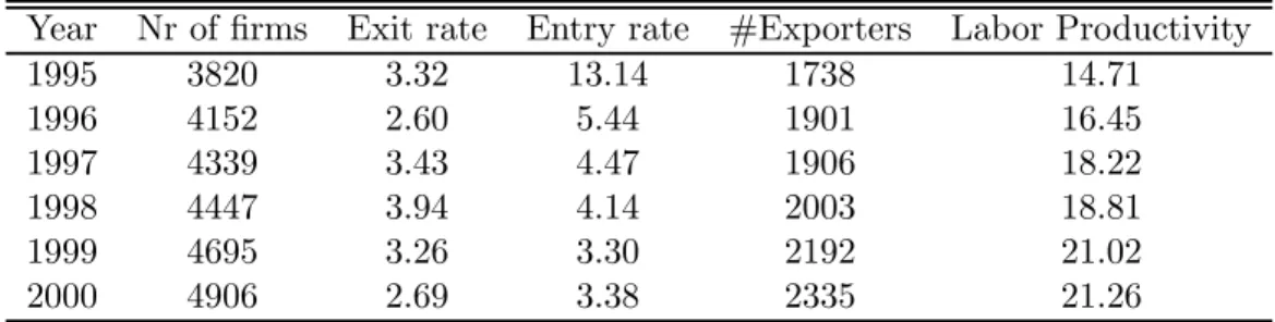
Table 1 provides some summary statistics about the industrial dynamics in our sample. While the annual average exit rate is around 3 percent, entry rates are very high, especially at the beginning of the period. This reflects new opportunities that were exploited after transition started.
Table 1: Firm Turnover and Exporting in Slovenian Manufacturing Year Nr of firms Exit rate Entry rate #Exporters Labor Productivity
1995 3820 3.32 13.14 1738 14.71 1996 4152 2.60 5.44 1901 16.45 1997 4339 3.43 4.47 1906 18.22 1998 4447 3.94 4.14 2003 18.81 1999 4695 3.26 3.30 2192 21.02 2000 4906 2.69 3.38 2335 21.26
Labor Productivity is expressed in thousands of Tolars.
Our summary statistics show labor productivity increased dramatically, consistent with the image of a Slovenian economy undergoing successful restructuring. At the same time, the number of exporters grew by 35 percent, taking up a larger share of total manufacturing both in total number offirms, as in total sales and total employment.
We use the detailed information on export status to shed some light on markup dif-ferences between exporters and domestic producers. We study the relationship between exports and markups since exports have gained dramatic importance in Slovenian man-ufacturing. We observe a 42 percent increase in total exports of manufacturing products over the sample period 1994-2000. Furthermore, entry and exit has reshaped market struc-ture in most industries. Both the entry of more productivefirms and the increased export participation was responsible for significant productivity improvements in aggregate (mea-sured) productivity (De Loecker and Konings, 2006 and De Loecker, 2007a). Therefore, we want to analyze the impact of the increased participation in international markets on the firms’ ability to charge prices above marginal cost.
1 6
We refer to De Loecker and Konings (2006) and De Loecker (2007a) for more details on the Slovenian data.
5
Markups and Firm Export Status Dynamics
We report our main results and discuss how our method provides substantially different markup estimates. We briefly discuss the importance of our suggested control function approach to answer important policy questions in the context of export entry.
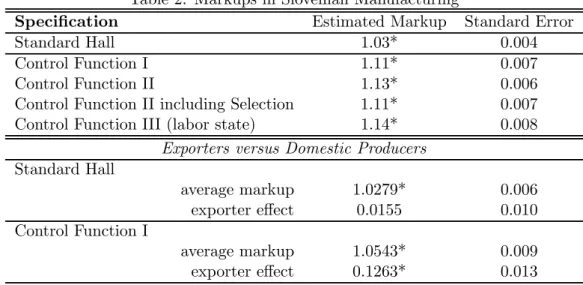
Table 2 collects our main findings. We estimate the markup under various specifi ca-tions: 1) the standard Hall approach, 2) various versions of our control function approach. For the latter we consider 4 different specifications: Control Function I simply introduces the control for productivity growth as introduced in section 2.5. Furthermore, we show the estimates using a second approach (Control Function II ) where we estimate the model without and with the selection correction. Finally, we estimate the markup allowing for adjustment cost in labor (Control Function III) which boils down to an ACF approach to correct for productivity (section 3.2).
Table 2: Markups in Slovenian Manufacturing
Specification Estimated Markup Standard Error
Standard Hall 1.03* 0.004
Control Function I 1.11* 0.007
Control Function II 1.13* 0.006
Control Function II including Selection 1.11* 0.007
Control Function III (labor state) 1.14* 0.008
Exporters versus Domestic Producers Standard Hall average markup 1.0279* 0.006 exporter effect 0.0155 0.010 Control Function I average markup 1.0543* 0.009 exporter effect 0.1263* 0.013
All regressions include time and industry dummies.
A robust finding is that the estimated markup is higher when we rely on the control function to proxy for unobserved productivity growth and the non random exit of firms. The interpretation of this finding is that input growth is negatively correlated with pro-ductivity growth. Firms that are experiencing positive propro-ductivity shocks can rely on the same (or less) inputs to produce more output.18 This is consistent with the transition
1 8We have to note that our approach is subject to the same concern as the estimation of production
function where deflated revenue is used to proxy for output. However, in our context unobserved growth in prices needs to be correlated with input growth, otherwise it will not affect our markup estimates. De
process wherefirms scaled down employment after long periods of labor hoarding, as well as the entry of de novo firms who enter at a much smaller scale.
In the lower panel we verify whether exportingfirms (on average) have higher markups (given that exporters tend to produce at lower marginal costs) and compare our results with the standard Hall approach.19 In order to estimate the markup for exporters we extend our main estimating equation and interact the relevant term,∆xit, with an exporter dummyEXPit.
∆qit =μD∆xit+μE∆xitEXPit+δEEXPit+∆φt(iit, kit) +∆εit
When we use the standard Hall specification, we cannot find significantly different markups for exporting firms20. On the contrary, our approach is better suited to an-alyze markups differences between exporters and non-exporters, since we can explicitly control for the export-productivity correlation in addition to the standard input growth-productivity growth correlation. Both correlations need to be controlled for in order to estimate a markup for domestic producers and exporters consistently. Indeed, when we control for unobserved productivity shocks, we find a significant higher markup for exporters. This result has important policy implications, as the well documented produc-tivity premium of exporters could be, at least partly, a consequence of pricing differences. We tested whether exporters’ (average) markup are different in the domestic (μE,D) and foreign market (μE,E) by decomposingμE∆xitEXPitinto(μE,DsDit+μE,EsEit)∆xitEXPit, where sDit and sEit are the share of domestic and foreign sales in total sales, respectively. Wefind only a slightly lower domestic markup (0.126), but not statistically different from the foreign market’s markup (0.132). In fact, using the firm specific shares, the average total export markup parameter is 0.131, compared to 0.1263 in Table 2.21
These results are consistent with the well established empirical fact that exporters are more productive. In the case of Slovenia, De Loecker (2007a)finds significant productivity differences between exporters and domestic producers. In addition, he finds that export entry further leads to productivity gains - often referred to as learning by exporting - in addition to the more productive firms self selecting into export markets. In the context
Loecker (2007b) shows that this is mostly severe for obtaining reliable measures for productivity. The coefficients on the inputs do hardly change when controlling for unobserved prices and demand shocks. Jaumaundreu and Mairesse (2006) document similarfindings using Spanish manufacturing data.
1 9
All the coefficients are robust to considering firms with positive investment only and thefore the difference between the uncorrected and corrected estimates are not driven by specific sample of firms. In Appendix B we report the estimated markups for the various industries.
2 0
A few papers analyzed this relationship using the Roeger method (Görg and Warzynski, 2003; Bellone et al., 2007),finding an export premium in markups as well. This paper provides a novel and moreflexible methodology.
2 1This test rests on an implicit assumption that the share of domestic (export) sales in total sales are
the correct weights, and implies that inputs are used proportional to sales. Without more detailed data on inputs by product or market, it is an open question how strong this assumption is.
of our model it is clear that, if we do not control for unobserved productivity shocks, the estimated interaction effect of export status and input growth - and therefore markups for exporters - is biased.22
So far we have just estimated differences in average markups for exporters and do-mestic producers. Our dataset also allows us to test whether markups differ significantly within the group of exporters. It is especially of interest to see whether there is a specific pattern of markups for firms that enter export markets, i.e. before and after they become an exporter. This will help us to better interpret the results from a large body of em-pirical work documenting productivity gains for new exporters. These results are used to confirm theories of self-selection of more productivefirms into export markets as in Melitz (2003) or learning by exporting. We now turn our attention to the various categories of exporters that we are able to identify in our sample: starters, quitters and firms that export throughout the sample period. To capture the relationship between how markups change as a firm enters or exits an export market, we run a similar regression interacting the markup with a firm-time specific export status variable, defined as a set of dummies,
statusit, as follows ∆qit = μ∆xit+statusit∗∆xit+∆φt(iit, kit) +∆εit (22) statusit = (μs,bBitst+μs,aAstit +μalALit+μq,bB q it+μq,aA q it)
In equation (22) Bitst is a dummy equal to 1 if thefirm starts exporting (we call these
firms ‘starters’) during our period of analysis, say at timetStart0 , and the observation takes place before it starts exporting (t < tStart0 ), and equal to 0 otherwise; Astit is equal to 1 if the firm starts exporting and we observe it after it started exporting (t≥ tStart0 ), and equal to 0 otherwise; ALit is equal to 1 if the firm is always exporting during our period of analysis, and 0 otherwise; Bitq is equal to 1 if the firm stopped exporting during the period (we refer to thesefirms as ‘quitters’), but is observed while it was still an exporter, and equal to 0 otherwise; Aqit is equal to 1 if the firm stopped exporting and is observed after it stopped exporting, and equal to 0 otherwise. The default category consists offirms producing only for the domestic market.
Table 3 shows the results and we clearly see that firms which are always exporting have a larger markup than firms that sell only on the domestic market, consistent with the evidence reported above.
A new set of results emerges in the rows two to six. Firms entering export markets have a larger markup even before they start exporting than their domestic counterparts.
2 2In the case where export status is a state variable in the underlying model we cannot identify the
interaction term in a first stage. This would imply that export status is part of the non parametric function φ(.). For a discussion on this see De Loecker (2007a).
Table 3: Markups and export dynamics (Control Function) Coefficient s.e.
Baseline (domestic) 1.04* 0.012
Starters Before Entering 0.08** 0.033
After Entering 0.15* 0.021
Always exporters 0.14* 0.020
Stopper Before Exiting 0.03 0.020
After Exiting -0.11* 0.030
Regression includes industry and year dummies in addition to separate dummy variables.
The latter is consistent with the self-selection hypothesis whereby more efficientfirmsfind it productive to pay the fixed cost of entering an export market. Here more efficient can mean that a domesticfirm might simply produce at a higher cost while charging the same price.
Interestingly, markups increase very substantially, on average, after export entry and the average markup increases to a level slightly above the markup of firms that continue exporting. The difference, however, is not significant.
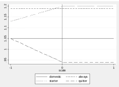
For firms that stop exporting, their markup did not deviate from the level of non-exporting firms when they were still exporting, but after they stop exporting, the markup drops dramatically.23 Figure 1 in Appendix A shows this evolution graphically. It is important to note that these patterns are not found when we do not control for unobserved productivity shocks, in fact markups are either insignificant or much lower in magnitude. The latter shows again the importance of controlling for the correlation between export status and productivity shocks.
It is striking to see that the markup-export patterns are identical to the productivity-export patterns found in De Loecker (2007a). He finds that productivity increases upon export entry and that exporters are more productive than their domestic counterparts. These results are suggestive of changes in performance of new exporters due to higher markups. Bringing this evidence together with the robust (revenue) productivity premia, at the very least requires a deeper investigation of what these measured productivity gains for exporters are suppose to capture. In addition, our evidence suggests that the gap between the notion of (physical) productivity in theoretical models like Melitz (2003) and the empirical measurement of productivity is an important one, i.e. markups are different for exporters and they change as firms switch status. We leave this for further research.
Finally, given our framework, we can back out estimates for productivity growth after
2 3
This could suggest that thesefirms were exporting poor quality products to Eastern European coun-tries.
we estimated the markup parameter.24 However, now we have to take a stand on the returns to scale - or implicitly on the user cost of capital - under which firms produce.25 It is clear from equation (5) that we can only compute implied productivity growth after imputing values forαKit. Let us return to the main estimating equation before introducing the use of the control function and consider productivity growth
∆qit−bμ(αLit∆lit+αM it∆mit+ (λit−αLit−αM it)∆kit) =∆ωdit (23)
We rely on our estimates of the markup bμ and impose various values for the returns to scale parameter λit. We consider three different cases where λit will take values of 1,
1.1 and 0.9 or constant, increasing and decreasing returns to scale. In this way we can compare the productivity growth estimates between the uncorrected approach(column I) and our control function approach (column II)under the three different cases. It is clear that using standard techniques will lead to biased estimates for productivity growth since they are based on downward biased markup estimates. Within the context of sorting out markup differences between exporters and domestic producers, the uncorrected approach would actually predict no differences in productivity growth, conditional on input use, between the two, which is clearly in contradiction with empirical evidence. Table 4 shows implied productivity growth under the various scenarios for both approaches.
Table 4: Implied Productivity Growth (Annual Averages in percentages)
CRS IRS DRS
I II I II I II
A) Manufacturing 3.52 2.16 3.01 1.58 4.03 2.75
B) Industry (weighted) 3.21 1.57 2.77 1.03 3.73 2.11 C) Manufacturing (status) 3.52 2.45 3.01 1.87 4.03 3.07
I is standard model without correction, II is control function approach.
We report productivity growth as simple average across allfirms in Slovenian manu-facturing (A), as an average of industry specific sales weighted productivity (B) and as an average obtained from regression (22) averaged over allfirms (C). The various comparisons in table 4 clearly show that productivity growth is overestimated without controlling for endogeneity of inputs and markup differences (column I). Indeed, productivity growth is roughly only half of what we obtain when we ignore these two effects (column II). The bias is not specific to the returns to scale we assume, however, the implied productivity estimates do depend on the values for λ.
2 4This is ruled out when relying on the Roeger (1995) method. 2 5
Note that we do not have to make any assumptions on returns to scale when estimating the markup parameter.
The last row shows productivity growth under our specification (22) where we allow for markups to change with a change in a firm’s export status. These effects are not present when we do not control for unobserved productivity shocks, and therefore the productivity growth estimates are exactly the same as in row (A). Although, our method is not intended to directly provide estimates for productivity growth, we see this as an important cross validation of the estimated markup parameters. Our estimates suggest average annual productivity growth rates for Slovenian manufacturing between 3 and 1.5 percent.
6
Discussion and Conclusion
This paper investigates the link between markups and exporting behavior. We find that markups differ between exporters and non exporters. In order to analyze this relationship we propose a simple andflexible methodology to estimate markups building on the seminal paper by Hall (1986) and the work by Olley and Pakes (1996). The advantages of our method are that we explicitly consider the selection process in the estimation and do not rely on the assumption of constant returns to scale and the need to compute the user cost of capital.
We use data on Slovenia to test whether i) exporters, on average, charge higher markups and ii) whether markups change forfirms entering and exiting export markets. Slovenia is a particularly interesting emerging economy to study as it has been successfully transformed from a socially planned economy to a market economy in less than a decade, reaching a level of GDP per capita over 65 percent of the EU average by the year 2000. More specifically, the sample period that we consider is characterized by considerably productivity growth and relative high turnover. Our methodology is therefore expected to find significantly different markups as we explicitly control for the non random exit offirms and unobserved productivity shocks. Our results confirm the importance of these controls.
Our method delivers higher estimates of firm-level markups compared to standard techniques that cannot directly control for unobserved productivity shocks. Our estimates are robust to various price setting models and specifications of the production function. We find that markups differ dramatically between exporters and non exporters, andfind significant and robust higher markups for exporting firms. The latter is consistent with thefindings of productivity premium for exporters, but at the same time requires a better understanding of what these (revenue based) productivity differences exactly measure. We provide one important reason for finding higher measured revenue productivity: higher markups. Furthermore, we estimate significant higher markups for firms entering export markets.
We see these results as a first step in opening up the productivity-export black box, and provide a potential explanation for the big measured productivity gains that go in hand with becoming an exporter. In this way our paper is related to the recent work of Constantini and Melitz (forthcoming) who provide an analytic framework that generates export entry productivity effects due tofirms making joint export entry-innovation choice, where innovation leads to higher productivity.
References
[1] Ackerberg, D., Benkard, L., Berry, S. and Pakes, A., 2007. "Econometric Tools for Analyzing Market Outcomes". in Handbook of Econometrics, Volume 6, 4173-4276. [2] Ackerberg, D., Caves, K., and Frazer, G., 2007. Structural Identification of Production
Functions, mimeo, UCLA.
[3] Berry, S., Levinsohn, L. and Pakes, A. 1995. Automobile Prices in Market Equilib-rium, Econometrica, 63, 841-890.
[4] Berry, S., Levinsohn, J. and Pakes, A. 2004, Estimating Differentiated Product De-mand Systems from a Combination of Micro and Macro Data: The Market for New Vehicles,Journal of Political Economy, vol. 112, no. 1,1, pp. 68-105.
[5] Basu, S., Fernald, J.G., 1997. Returns to Scale in U.S. Production: Estimates and Implications, Journal of Political Economy, 105, 249-83.
[6] Bellone, F., Musso, P., Nesta, L. and Warzynski, F., 2008. Endogenous Markups, Firm Productivity and International Trade, mimeo, OFCE.
[7] Constantini, J. and Melitz, M. Forthcoming. The Dynamics of Firm-Level Adjustment to Trade Liberalization, in Helpman, E., D. Marin, and T. Verdier, The Organization of Firms in a Global Economy, Harvard University Press, 2008.
[8] De Loecker, J. and Konings, J. 2006, Job Reallocation and Productivity Growth in an Emerging Economy,European Journal of Political Economy, vol 22, pp. 388-408. [9] De Loecker, J. 2007a. Do Export Generate Higher Productivity? Evidence from
Slovenia. Journal of International Economics, 73, 69—98.
[10] De Loecker, J. 2007b. Production Differentiation, Multi-Product Firms and Estimat-ing the Impact of Trade Liberalization on Productivity, NBER WP # 13155.
[11] Domowitz, I. Hubbard, R.G. and Petersen, B.C. 1988. Market Structure and Cyclical Fluctuations in U.S. Manufacturing, The Review of Economics and Statistics, Vol. 70, No. 1., pp. 55-66.
[12] Foster, L., Haltiwanger, J. and Syverson, C., 2008. Reallocation, Firm Turnover, and Efficiency: Selection on Productivity or Profitability? American Economic Review, 98 (1), 394-425.
[13] Goldberg, P. 1995. Product Differentiation and Oligopoly in International Markets: The Case of the U.S. Automobile Industry,Econometrica, Vol. 63, No. 4, pp. 891-951.
[14] Görg, H. and Warzynski, F., 2003. The Dynamics of Price Cost Margins and Export-ing Behaviour: Evidence from the UK. LICOS Discussion Paper # 133.
[15] Hall, R.E., 1986. Market Structure and Macroeconomic Fluctuations. Brookings Pa-pers on Economic Activity 2, 285-322.
[16] Hall, R. E., 1988. The Relation between Price and Marginal Cost in U.S. Industry. Journal of Political Economy 96 (5), 921-947.
[17] Hall, R. E., 1990. Invariance Properties of Solow’s Productivity Residual, in Di-amond, P. (ed.), Growth, productivity, Unemployment: Essays to celebrate Bob Solow’s Birthday, Cambridge, MA: MIT Press, 71-112.
[18] Halpern, L., Koren, M. and Szeidl, A. 2006. Imports and Productivity, mimeo CEU, Budapest.
[19] Harrison, A., 1994. Productivity, Imperfect Competition, and Trade Reform: Theory and Evidence,Journal of International Economics 36, 53-73.
[20] Jaumaundreu, J. and Mairesse, J. (2006), Using price and demand information to identify production functions, mimeo, CREST.
[21] Kasahara, H. and Rodrigue, J., 2008. Does the use of imported intermediates increase productivity? Plant-level evidence,Journal of Development Economics, 87, 106-118. [22] Klette, T. J. , 1999. Market Power, Scale Economies and Productivity: Estimates from a Panel of Establishment Data. Journal of Industrial Economics 47 (4), 451-476.
[23] Klette, T. J. and Griliches, Z., 1996. The Inconsistency of Common Scale Estimators When Output prices Are Unobserved and Endogenous,Journal of Applied Economet-rics 11 (4), 343-361.
[24] Konings, J., Van Cayseele, P. and Warzynski, F. 2005. The Effect of Privatization and Competitive Pressure on Firms’ Price-Cost Margins: Micro Evidence from Emerging Economies. The Review of Economics and Statistics 87 (1), 124-134.
[25] Konings, J. and Vandenbussche, H., 2005. Antidumping protection and markups of domesticfirms, Journal of International Economics, 65 (1), 151-165.
[26] Krishna, P. and Mitra, D., 1998. Trade liberalization, market discipline and produc-tivity growth: new evidence from India. Journal of Development Economics 56 (2), 447-462.
[27] Levinsohn, J., 1993. Testing the imports-as-market-discipline hypothesis, Journal of International Economics, 35, 1-21.
[28] Levinsohn, J. and Petrin, A., 2003. Estimating Production Functions Using Inputs to Control for Unobservables. Review of Economics Studies 70, 317-340.
[29] Lööf, H. and Andersson, M., 2008. Imports, productivity and the origin markets - the role of knowledge-intensive economies, working paper, CESIS.
[30] Melitz, M. 2003. The Impact of Trade on Intra-Industry Reallocations and Aggregate Industry Productivity,Econometrica, Vol. 71, November 2003, pp. 1695-1725. [31] Melitz, M. and Ottaviano, G. 2008. Market Size, Trade, and Productivity, Review of
Economic Studies, Vol. 75, January 2008, pp.295-316.
[32] Morrison, C.J. 1992. Unraveling the Productivity Growth Slowdown in the United States, Canada and Japan: The Effects of Subequilibrium, Scale Economies and Markups, The Review of Economics and Statistics, Vol. 74, No. 3. (Aug., 1992), pp. 381-393.
[33] Norrbin, S. C., 1993. The Relation between Price and Marginal Cost in U.S. Industry: A Contradiction,Journal of Political Economy 101, 1149-1164.
[34] Olley, S. G. and Pakes, A, 1996. The Dynamics of Productivity in the Telecommuni-cations Equipment Industry,Econometrica 64 (6), 1263-1297.
[35] Petrin, A. 2002. Quantifying the Benefits of New Products: The Case of the Minivan, Journal of Political Economy , 110, 705-729.
[36] Roeger, W., 1995. Can Imperfect Competition Explain the Difference between Pri-mal and Dual Productivity Measures? Estimates for U.S. Manufacturing. Journal of Political Economy 103(2), 316-330.
[37] Shapiro, M., 1987. Measuring Market Power in US Industry. NBER WP # 2212. [38] Van Biesebroeck, J., 2005. Exporting Raises Productivity in sub-Saharan African
Manufacturing Firms,Journal of International Economics, 67 (2), 373-391
[39] Waldmann, R. J., 1991. Implausible Results or Implausible Data? Anomalies in the Construction of Value-Added Data and Implications for Estimates of Price-Cost MarkupsJournal of Political Economy 99, 1315-1328
.9 5 1 1. 0 5 1. 1 1. 15 1. 2 -1 0 1 scale
domestic alw ays starter qui tter
Figure 1: Export-Markup Dynamics in Slovenian Manufacturing.
Appendix A: Multi-Product Firm Bertrand Price Setting and Markups Suppose as in Berry, Levinsohn and Pakes (1995) that there areF firms in a specific industries, producing differentiated products. Each firm produces a subset Γf of the J products available on the market. To understand what our markup estimates refer to in the context of this model, let us look at the short run profit function offirm f:
Πf = X j∈Γf (pj−mcj)qj = X j∈Γf (pj−mcj)M sj(p, x, ξ;ϑ)
whereM is the size of the market andsis market share, that depends on the price vector, as well as observed (x) and unobserved characteristics (ξ) of the products (ϑis the vector of parameters to be estimated).
Maximizing profits with respect to price, we get the following FOC:
sj(p, x, ξ;ϑ) + X j∈Γf (pj−mcj) ∂sj(p, x, ξ;ϑ) ∂pj = 0
βf = p−mc p = s(p, x, ξ;ϑ) p 1 ∆(p, x, ξ;ϑ)
where ∆rj is a JxJ matrix whose (j,r) element is defined by:
∆rj =
∂sj(p,x,ξ;ϑ)
∂pj ifr and j are produced by the same firm 0otherwise
In other words, the markup is a function of the sensitivity of market share to price, given the set of prices set by competitors, the characteristics of all products on the markets and the characteristics of the consumers on the market.
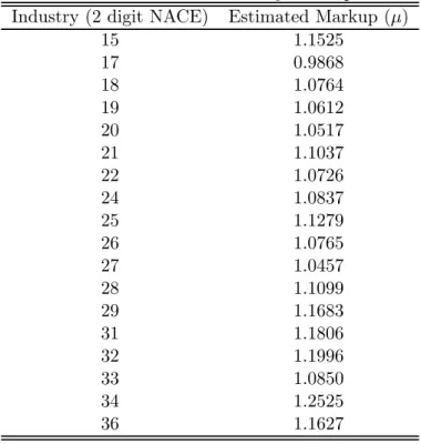
Appendix B: Industry Markups and Export Dynamics
We report the estimated markup coefficients for the various industries of the Slovenian manufacturing sector. These coefficients are obtained after running the exact same re-gression as in Table 2 (upper panel) by industry to free up the markup parameter. This robustness check shows that our results are not specific to certain sectors or aggregation.
Table 5: Estimated Industry Markups Industry (2 digit NACE) Estimated Markup (μ)
15 1.1525 17 0.9868 18 1.0764 19 1.0612 20 1.0517 21 1.1037 22 1.0726 24 1.0837 25 1.1279 26 1.0765 27 1.0457 28 1.1099 29 1.1683 31 1.1806 32 1.1996 33 1.0850 34 1.2525 36 1.1627