Local labor market effects of public employment [WP]

(1)

LOCAL LABOR MARKET EFFECTS OF PUBLIC EMPLOYMENT

Jordi Jofre-Monseny, José I. Silva, Javier Vázquez-Grenno

Document de treball de l’IEB

2016/11

(2)

Documents de Treball de l’IEB 2016/11

LOCAL LABOR MARKET EFFECTS OF PUBLIC EMPLOYMENT

The

IEB

research program in

Cities and Innovation

aims at promoting research in the

Economics of Cities and Regions. The main objective of this program is to contribute to

a better understanding of agglomeration economies and 'knowledge spillovers'. The

effects of agglomeration economies and 'knowledge spillovers' on the Location of

economic Activities, Innovation, the Labor Market and the Role of Universities in the

transfer of Knowledge and Human Capital are particularly relevant to the program. The

effects of Public Policy on the Economics of Cities are also considered to be of interest.

This program puts special emphasis on applied research and on work that sheds light on

policy-design issues. Research that is particularly policy-relevant from a Spanish

perspective is given special consideration. Disseminating research findings to a broader

audience is also an aim of the program. The program enjoys the support from the

IEB-Foundation.

The

Barcelona Institute of Economics (IEB)

is a research centre at the University of

Barcelona (UB) which specializes in the field of applied economics. The

IEB

is a

foundation funded by

the following institutions: Applus, Abertis, Ajuntament de

Barcelona, Diputació de Barcelona, Gas Natural, La Caixa and Universitat de

Barcelona.

Postal Address:

Institut d’Economia de Barcelona

Facultat d’Economia i Empresa

Universitat de Barcelona

C/ John M. Keynes, 1-11

(08034) Barcelona, Spain

Tel.: + 34 93 403 46 46

ieb@ub.edu

http://www.ieb.ub.edu

The IEB working papers represent ongoing research that is circulated to encourage

discussion and has not undergone a peer review process. Any opinions expressed here

are those of the author(s) and not those of IEB.

(3)

Documents de Treball de l’IEB 2016/11

LOCAL LABOR MARKET EFFECTS OF PUBLIC EMPLOYMENT

*

ABSTRACT:

This paper quantifies the impact of public employment on local labor

markets in the long-run. We adopt two quantitative approaches and apply them to the case

of Spanish cities. In the first, we develop a 3-sector (public, tradable and non-tradable)

search and matching model embedded within a spatial equilibrium model. We characterize

the steady state of the model, which we calibrate to match the labor market characteristics

of the average Spanish city. The model is then used to simulate the local labor market

effects of expanding public sector employment. In the second empirical approach, we use

regression analysis to estimate the effects of public sector job expansions on decadal

changes (1980-1990 and 1990-2001) in the employment and population of Spanish cities.

This analysis exploits the dramatic expansion of public employment that followed the

advent of democracy in the period 1980 to 2001. The instrumental variables’ approach that

we adopt uses the capital status of cities to instrument for changes in public sector

employment. The two empirical approaches yield qualitatively similar results and, thus,

cross-check each other. One additional public sector job creates about 1.3 jobs in the private

sector. However, these new jobs do not translate into a substantial reduction in the local

unemployment rate as better labor market conditions attract new workers to the city.

Increasing public employment by 50% only reduces unemployment from 0.156 to 0.150.

JEL Codes: J45, J64, H70, R12

Keywords: Public employment, search, local multipliers, unemployment

Jordi Jofre-Monseny

Universitat de Barcelona & IEB

Av. Diagonal 690

08034 Barcelona, Spain

Email:

jordi.jofre@ub.edu

José I. Silva

Universitat de Girona

Campus de Montilivi

17071 Girona, Spain

Email:

jose.silva@udg.edu

Javier Vázquez-Grenno

Universitat de Barcelona & IEB

Av. Diagonal 690

08034 Barcelona, Spain

Email:

jvazquezgrenno@ub.edu

(4)

1 Introduction

Public employment constitutes a significant fraction of employment. In 2013, the share of public employment in total employment was, on average, 21% in OECD countries1. Hence, policies regarding public sector wages and employment are likely to influence the labor market. The objective of this study is to estimate the long-run labor market effects of public employment at the city-level.

There is evidence from different countries indicating that governments use public employ-ment as a policy tool to affect local labor market performance. Specifically, governemploy-ments use the distribution of public employment within their countries’ geography as a means to reduce spatial economic inequalities. In 1992, up to 400,000 jobs in public works in East Germany cush-ioned the rise in unemployment that followed re-unification (Kraus et al.,1998). In Spain, jobs in public works have been created in rural and lagging areas as a means to increase local disposable income (Jofre-Monseny,2014). In Sweden, the creation of universities in less prosperous cities has formed part of the country’s regional policy to reduce regional economic disparities ( Ander-sson,2005). In England, 25,000 public sector jobs were relocated away from London between 2004 and 2010. Among other objectives, the policy aimed at stimulating economic activity in less prosperous areas (Faggio and Overman,2014). Less explicitly, interregional income redistribu-tion has partly been achieved through a higher concentraredistribu-tion of public sector jobs in the south, both in Italy (Alesina et al., 2001) and in Spain (Marqués-Sevillano and Rosselló-Villallonga, 2004). Focusing on risk sharing between Norwegian regions, Borge and Matsen(2004) show that public employment is a prominent force for counterbalancing local economic shocks.

Increasing the number of public employees in a city increases the demand for local services such as housing, restaurants and hair-dressers, crowding-in private employment. However, this effect may be offset by increases in local wages and prices that might follow the public em-ployment expansion. This crowding-out effect can be particularly acute in the tradable sector since local workers do not significantly affect the demand for locally produced manufactures. In addition, local job creation can increase in-migration rates, which might also weaken the link between more jobs in the local economy and a lower unemployment rate among its residents.

To quantify the long-run local labor market effects of public employment, we adopt two quantitative approaches that we apply to the case of Spanish cities. In the first, we calibrate and simulate a search and matching model with geographically mobile workers. In the second, we resort to regression analysis. These two empirical approaches yield qualitatively similar results and, thus, cross-check each other.

We first develop a 3-sector (public, tradable and non-tradable) search and matching model à laDiamond(1982)-Mortensen (1982)-Pissarides(1985). The model assumes that (homoge-neous) workers only search for work when are unemployed and that they accept any job offered.

(5)

Moreover, unemployed workers can move at zero cost. It is assumed that each city is sufficiently small, implying a fixed reservation utility for the unemployed. Workers consume all their in-come on a tradable good, a non-tradable good and land. The latter two prices are endogenous and clear their respective markets while the price of the tradable good is exogenous and deter-mined in the national (or international) market. Due to geographical mobility, a city whose labor market prospects improve is a city that must become more expensive to live-in. Vacancies and wages in the public sector are exogenously determined while, in the private sector, free-entry means that firms in the tradable and non-tradable sectors open up vacancies until the expected value becomes zero.

We characterize the steady state of the model, which we then calibrate to match the labor market characteristics of the average Spanish city. Then, we use the model to simulate the lo-cal labor market effects of expanding public sector employment. The geographilo-cal mobility of workers implies that the labor force in the city increases with public sector job expansion. In the non-tradable sector, the wage increase resulting from the policy is clearly offset by the rise in local demand for the non-tradable good, and employment in this sector increases substan-tially. In contrast, the demand for the locally produced tradable good remains unaffected. As a result, the effect on tradable employment is small, being determined by two opposing forces: higher wages, on the one hand, decrease employment, while agglomeration economies, on the other, which boost productivity, increase employment. In our baseline calibration, one addi-tional public sector job increases private jobs by 1.3 and the workforce by 2.6 individuals. As a result, large expansions in public employment have only modest impacts on the local un-employment rate. Increasing public un-employment by 50% only reduces the unun-employment rate from 0.156 to 0.149.

In the second empirical approach, we use regression analysis to estimate the effects of public sector job expansions on decadal changes (1980-1990 and 1990-2001) in the employment and population of Spanish cities. This analysis exploits the dramatic increase in public employment that followed the advent of democracy after Franco’s death. Between 1980 and 2001, public employment grew by 133%, increasing from 1.4 to 3.2 million jobs. We start by analyzing the determinants of this public sector job expansion across cities. Two important results emerge. First, more public sector jobs were created in cities experiencing negative labor demand shocks, providing further evidence that public employment is used by governments to reduce spatial income inequalities. Second, the provincial capitals (established in 1833) experienced a more than proportionate increase in public employment between 1980 and 2001. Specifically, being a capital city implied an additional 1.6 public sector jobs each decade per 100 inhabitants in the base year. This result is the basis for our Two Stage Least Squares (TSLS) strategy which consists in using the capital status of cities to instrument for changes in public sector employment. As for instrument validity, several robustness checks support the assumption made that (conditional

(6)

on initial unemployment, education, location -coast versus inland cities- and size) the capital status of a city is uncorrelated to shocks in employment and population growth. The TSLS esti-mates also indicate that one additional public sector job increases private jobs by about 1.3 and the labor force by 2.7 individuals. The reduced-form estimates obtained imply that increasing public employment by 50% only reduces the unemployment rate from 0.156 to 0.150.

There are, at least, three factors that serve to rationalize the relatively large multipliers that we find. First, in the period that we study (1980-2001), interregional migration rates in Spain were relatively low but, in contrast, intraregional migration rates were substantial (Bover and Arellano, 2001). Specifically, cities continued to attract migrants from the rural areas within their region and more public sector jobs in the capital cities might have intensified this process. Second, the model simulations indicate that land supply elasticity is critical in determining if, and the extent to which, public employment crowds-in or crowds-out private employment. The complier cities in our TSLS regressions are relatively small provincial capitals which can be con-sidered as being cities with a rather elastic land supply. Finally, our model also indicates that multipliers are greater when public sector wages are high. In Spain, the public sector wage gap is substantial (Hospido and Moral-Benito,2014), and this is especially true in small provincial capitals given that the distribution of public sector wages is more compressed than that of the private sector.

The paper that is closest to ours isFaggio and Overman(2014), who estimate the local la-bor market effects of public employment in England. Their main results, based on 2003-2007 employment changes at the English Local Authority level, indicate that public employment nei-ther increases nor decreases overall private employment, although the industry mix is changed in favor of the non-tradable sector. When examining a longer time horizon (1999-2007), their results suggest that, if anything, public employment crowds-out rather than crowds-in private employment. AsFaggio and Overman(2014) recognize, the highly restrictive planning system prevalent in England (Hilber and Vermeulen,2015) implies a very inelastic land (and housing) supply which could explain the absence of significant crowding-in effects on private employ-ment in that country. We compleemploy-ment the study conducted byFaggio and Overman(2014) in several ways. First, we estimate the local labor market effects of public employment in Span-ish cities. For the reasons detailed above, these estimates can be policy-relevant in settings with unrestrictive planning systems and/or with favorable geography for urban development. Second, we study a time period in which the Spanish public sector developed, with massive, geographically heterogeneous increases in public employment. While in the period studied by Faggio and Overman(2014), public employment in England increased by less than 6%, in our setting there was an increase of 133%. Third, we develop a search and matching model with geographical mobility that clarifies the mechanisms through which public employment affects cities and quantifies their relative importance. Finally, another attractive feature of our study

(7)

is the novel TSLS strategy that we use. Instead of using aBartik(1991) shift-share instrument that uses employment in the base year to predict subsequent employment growth, we use a city feature (the capital status of a city) that dates back to 1833 to predict public employment growth in the decades of 1980-1990 and 1990-2001. As we document that more public jobs are created in cities experiencing negative labor demand shocks, building a shift-share instrument with the 1980 and 1990 distribution of public employment could be problematic as these distributions may reflect past labor demand shocks, which are likely to be correlated over time.

Instead of analyzing the local labor market effects of public employment,Moretti(2010) and Moretti and Thulin(2013) estimate the local multipliers of jobs in the tradable sector in the US and Sweden, respectively. Their results indicate that, on average, one additional job in the tradable sector creates about 1.6 and 0.5 jobs in the non-tradable sector in the typical US and Swedish city, respectively. Our results, therefore, lie in between these two estimates, but are closer to the US multipliers.

Beaudry et al.(2012),Kline and Moretti(2013) embed standard search and matching models à la Diamond-Mortensen-Pissarides in spatial equilibrium models (Roback, 1982)2. Beaudry et al.(2012) set-up a multi-sector, multi-city model with labor market frictions. The empirics of the paper, which examines changes in wages and employment across cities and industries in the US, indicate that a positive labor demand shock in one sector increases wages in the rest of the city’s industries, providing empirical support for labor market frictions and bargaining. In a similar vein,Kline and Moretti(2013) examine the efficiency of place-based policies in the presence of geographical mobility and labor market frictions. In relation to these studies, we go a step further by calibrating the model and using it to simulate the effects of a local labor market policy. To the best of our knowledge, we are the first to do so in the context of search and matching models with geographical mobility.

Finally, our paper also relates to a recent strand of the macro literature studying the labor market effects of public employment in national economies. Burdett (2012), Gomes(2015a) andBradley et al.(2015) use search and matching models to analyze the effects of public sec-tor wages and employment on labor market performance3. The conclusions reached regarding the effects of public employment are much more negative than those obtained in the present study.Algan et al.(2002) also study the effects of public employment at the national level using regression analysis applied to a long OECD country-level panel. Their results also suggest strong crowding-out effects. Specifically, they indicate that one public job crowds-out 1.5 private sec-tor jobs and increases the number of unemployed by 0.3 individuals. Our study differs from this strand of the literature in that it estimates the effects at the city (rather than at the national) level.

2_{A related study is}_Wrede₍₂₀₁₅_{), which extends the urban economics literature on the measurement of quality}

of life by considering the presence of unemployment.

3_{Quadrini and Trigari}₍₂₀₀₇_{) and}_Gomes₍_2015b_{) are concerned instead with the effect of public employment}

(8)

Two facts can reconcile our results with those of this literature. First, labor mobility across cities implies that labor supply is much more elastic at the city than at the national level. In fact, in our search and matching model, if we consider the case with no geographical mobility, public employment also crowds-out private employment. Second, at the city level, the public wage bill is not financed through local taxes as it is typically financed by some upper-tier government.

The remainder of this paper is organized as follows. In section 2 we develop the theoretical model. Section 3 presents the calibration of the model (3.1) and the main results of the model simulations (3.2). Section 4 contains the regression analysis. We describe the data and variables (4.1) before providing the institutional background and analyzing the city-level determinants of the public sector job expansion (4.2). Then, we turn to a descriptive (Ordinary Least Squares) analysis of the effects of public employment on the city’s private employment and population (4.3) before proceeding to the main TSLS analysis (4.4). The effects of public employment on the local unemployment rate are addressed in section 4.5 and, finally, section 5 concludes.

2 The model

In this section we develop a search and matching model à la Diamond-Mortensen-Pissarides embedded within a spatial equilibrium model followingBeaudry et al. (2012) and Kline and Moretti(2013). Homogeneous workers can be either employed or unemployed. Employees can be either in the public sector (g), in the tradable sector (t) or in the non-tradable sector (n). Workers consume all their income on a tradable good, a non-tradable good and land. Unem-ployed workers can leave the city at no cost.

2.1 Employment and unemployment

Unemployed workers search for jobs in the three sectors simultaneously and enjoy the non-labor incomeb. We assume that the public sector is frictionless and job vacancies are instanta-neously filled. We assume that the public sector wage bill is not financed through local taxation since the lion’s share of this expenditure is financed by central and regional governments. We further assume that the public sector job creation rate (fg), separation rate (sg) and wage (wg),

are all exogenously determined. In the private sector, jobs are filled via a constant returns to scale matching function,m(uL,vL)=mouχv(1−χ)L, whereu is the unemployment rate,v the

vacancy rate andL is the labor force of each city, while χandmo are the elasticity and scale

matching function parameters, respectively. Unemployed workers find jobs in the tradable and non-tradable sectors at the endogenous ratesfi(θ)=m(uL_uL,vL) Ωi, whereΩi represents the

frac-tion of vacant jobs in each sector withi =t,n, i.e. Ωi = _v_tv₊i_v_n. In turn, vacancies in the

(9)

in the city (vacancies-unemployment ratio),θ≡ vt+vn

u ≡ v

u4. According to the properties of the

matching function, the higher the number of vacancies with respect to the number of unem-ployed workers, the easier it is to find a job,f0(θ)>0, and the more difficult it is to fill a vacancy,

q0(θ)<0.

The jobs in the tradable and non-tradable sectors can be either filled or vacant. Before a po-sition is filled, the firm has to open a job vacancy with a flow costki. Private firms have a

technol-ogy with labor as the only input. Each filled job in the tradable sector yields instantaneous profit equal to the difference between the marginal productivity of labor and the wage. The price of the tradable good is exogenous and normalized to one as tradable goods are sold in national (or international) markets, implying that the instantaneous profit amounts toAt(L)−wt. We

con-sider that productivity increases with city size due to agglomeration economies5. Specifically, the marginal productivity of labor is given by At(L)= At0Lζ, where 0<ζ<1 and At0 captures the exogenous technological level in the tradable sector. In turn, the instantaneous profit of the non-tradable sector is equal topn−wn, which increases with the (endogenous) price of the

non-tradable good,pn6. Employed workers in the tradable and non-tradable sectors separate

from their firm at the (sector-specific) constant ratesi.

Thus, the value of vacancies Vt andVn, and the value of a job in the tradable and

non-tradable sectors,Jt andJn, are represented by the following Bellman equations:

r Vt = −kt+q(θ)(Jt−Vt), (1)

r Vn = −kn+q(θ)(Jn−Vn), (2)

r Jt = At(L)−wt+st(Vt−Jt), (3)

r Jn = pn−wn+sn(Vn−Jn). (4)

Firms in the tradable and non-tradable sectors will open vacancies until the expected value of vacancies becomes zero. Thus, the free entry condition in these two sectors are:

r Vt = 0, (5)

4_{By the homogeneity of the matching function this ratio is not a function of}_L_.

5_See_{Combes and Gobillon}₍₂₀₁₅_{) for a recent review of the empirics of agglomeration economies.}

6_{We do not consider agglomeration effects in the non-tradable sector as there is less room for productivity}

(10)

r Vn = 0. (6)

2.2 Workers

Each worker consumes a tradable and a non-tradable good, and land. Hence, a worker’s utility in a city depends on their nominal income, y ={b,wg,wt,wn} as well as on the city’s prices

of the non-tradable good (pn) and land (pc)7. We assume that workers have a Cobb-Douglas

utility function which delivers indirect utilityV(y,pn,pc)=y

¡ 1−φ−δ¢(1−φ−δ) ³_φ pn ´φ³ δ pc ´δ = _Py, definingP as the city’s price index8.

P = µ 1 1−φ−δ ¶(1−φ−δ)µ pn φ ¶φ ³p_c δ ´δ . (7)

The parameters φand δreflect workers’ preferences for the non-tradable good and land, respectively, as well as being the income shares spent on these two goods. The values for unem-ployment (U) and employment in the public (Wg), tradable (Wt) and non-tradable (Wn) sectors

are given by the following expressions:

rU = b P +fg(Wg−U)+ft(Wt−U)+fn(Wn−U), (8) r Wg = wg P +sg(U−Wg), (9) r Wt = wt P +st(U−Wt), (10) r Wn = wn P +sn(U−Wn). (11)

We assume that unemployed individuals can move to another city at zero cost, implying that the utility of unemployed workers is equalized across cities. Since we assume that each city is

7_{Note that we do not consider non-participation in the labor market. As the regression results in section 4 show,}

the results do not indicate that public employment in a city increases labor force participation.

8_{In our model, having more public employees in the city does not increase the provision of local public goods}

and services and, thus, it does not increase city amenities. We take this modeling approach because, as will be-come clear below, public employees in capital cities provide public goods and services (administrative services, universities and hospitals) that clearly do not only benefit the city’s residents.

(11)

small relative to the whole economy, the value of unemployment is fixed atz. Alternatively, if we consider intraregional migrations between the city and its hinterland,zwould be the utility level achieved in the city’s hinterland.

rU = z, (12)

Taking equations8and12implies that, in equilibrium, if the labor market prospects of a city improve (high wages, high job finding rates and/or low job separation rates), then the city must become a more expensive place to live-in (higher price index).

The next assumption is that wages in the tradable and non-tradable sectors are set through Nash bargaining. The Nash solution is the wage that maximizes the weighted product of the worker’s and firm’s net return from the job match. The first-order condition from this maxi-mization problem is9:

1

PβJt=(1−β)(Wt−U), (13)

1

PβJn=(1−β)(Wn−U), (14)

where the parameterβrepresents the worker’s bargaining power.

To fully characterize the dynamics of this economy, we need to define the law of motion for the unemployment rate (u), and for the employment rates in the public (eg), tradable (et) and

non-tradable (en) sectors. These evolve according to the following differential equations:

˙ u = sg eg+stet+snen−fg u−ftu−fnu, (15) ˙ eg = fg u−sg eg, (16) ˙ et = ftu−st et, (17) ˙ en = fnu−snen, (18)

(12)

eg+et+en+u=1. (19)

Notice that the levels of unemployment and employment in the public, tradable and non-tradable sectors areuL,egL,etLandenL, respectively.

In order to close the model, the markets for the non-tradable good and land must clear. The non-tradable good must be purchased by local workers.

φ(wgeg+wtet+wnen+b u)=pnen. (20)

Finally, we assume that land rents accrue to absentee land owners and, followingCombes et al.(2012), we assume that land price is increasing with city size according to:

pc = Lη. (21)

2.3 Equilibrium

In equilibrium, the system of equations can be reduced to the following twelve key equations that characterize the behavior of the endogenous variablesθ, ft, fn,pn,pc,wt,wn,et,en,L, At

andu: kt q(θ) = At(L)−wt (r+st) , (22) kn q(θ) = pn−wn (r+sn) , (23) wt = βAt(L)+ ¡ (1−β)b+βθ(Ωtkt+Ωnkn) ¢ (r+sg) (r+sg+fg)+ fg(1−β)wg (r+sg+fg) , (24) wn = βpn+ ¡ (1−β)b+βθ(Ωtkt+Ωnkn) ¢ (r+sg) (r+sg+fg)+ fg(1−β)wg (r+sg+fg) , (25) u= sgstsn [stsnsg+sgstfn+sgftsn+fgstsn] , (26)

(13)

eg= fg sg u, (27) et= ft st u, (28) eg+et+en+u=1, (29) 1 P · b+ fg (r+sg+fg) (wg−b)+ (r+sg)βθ(Ωtkt+Ωnkn) (r+sg+fg)(1−β) ¸ = z, (30) φ(wgeg+wtet+wnen+b u)=pnen, (31) pc = Lη, (32) At(L)=At0L ζ_. ₍₃₃₎

Equations22and23are the standard job creation curves that characterize the marginal con-dition for the demand of labor in the tradable and non-tradable sectors, respectively. More jobs are created if wages, vacancy costs and labor market tightness are low and if marginal revenue (At(L) orpn) is high. Equations24and25are the respective wage curves that replace the labor

supply curves of Walrasian models (Pissarides(2000), page 17)10. As inBeaudry et al.(2012), frictions and bargaining result in wages in the private sector that depend on the wage and on the job finding and job separation rates in the public sector11. In turn, equations26to29 char-acterize the unemployment rate and the employment rates in the public, tradable and non-tradable sectors in steady state. Equations30, 32and33 appear as a consequence of workers’ mobility. Equation30relates the unemployment value (z) to the city’s land price and job mar-ket prospects, while32and33specify the rate at which the land price and productivity in the tradable sector increase with city size. Finally, equation31guarantees that the local price of the non-tradable good clears the market.

10_{The derivation of equations}₂₄_and₂₅_{are provided in Appendix}_B_. 11_{If there is no public employment (}_f

g=sg=0), the wage equations reduce to their standard form (Pissarides

(14)

3 Calibration and simulated results of the model

3.1 Calibration

We calibrate the model to match the labor market characteristics of the average Spanish city with transition rates defined at quarterly frequencies. Table1 summarizes all the calibrated parameters and presents the steady state values of the endogenous variables. The real interest rate is fixed at r =0.012, which is consistent with an annual interest rate of 4.8%. We target the 2001 city averages in terms of the unemployment rate (15.6%) and the employment rates in the public sector (20.9%), the tradable sector (15.8%) and the non-tradable sector (47.7%). Using the Spanish Labor Force Survey (SLFS) and adopting the methodology applied inSilva and Vázquez-Grenno(2013), we calculate the separation rates in the three sectors considered. While the separation rate in the public sector is sg =0.009, in the tradable and non-tradable

sectors these rates are higher and virtually identical withst =sn=0.015. Combining the job

separation rates, the employment rates and the unemployment rate with ˙eg =e˙t =e˙n=u˙=0

delivers the job finding ratesfg =0.012,ft=0.015 andfn=0.046.

Since we do not observe vacant jobs, to calibrate the model, we assume that the fraction of job vacancies in each of the two private sectors (Ωi) is given by the observed employment shares.

Thus, we setΩt =0.249 andΩn=0.751. This implies that the aggregate job finding rate in the

private sector isf =ft+fn=0.061. We normalize the labor market tightness to one,θ=1. Once

Ωn,u andθare known, we obtain the vacancy rates for the tradable and non-tradable sectors

usingΩn = _v_tv₊n_v_n andθ= vt+_uvn. We obtainvt =0.039 andvn=0.117 and, thus,v =vt+vn=

0.156. Finally, the vacancy filling rate isq(θ)= f_θ(θ) =0.061. Pissarides and Petrongolo(2001) identify the matching function elasticity parameter as being in the 0.5-0.7 range. We take 0.6 as our reference and, thus, we setχ=0.6. Given that we know the job finding rates andθ, we can then usef =moθ1−χto obtain the matching function scale parametermo=0.061.

As for wages, we normalize the wage in the public sector to one (wg =1). FollowingHospido

and Moral-Benito(2014), we target a wage gap of 20% between the public and private sectors. Similarly, we estimate the wage gap between the tradable and the non-tradable sectors using the Spanish Continuous Sample of Working Lives in 2005 (Muestra continua de Vidas Laborales, MCVL). We find a gap of 11.9% after controlling for individual characteristics (age, age square, gender and education), leaving us withwt =0.913 andwn=0.807.

According to Eurostat, labor productivity in the Spanish tradable sector was 45.7% higher than personnel costs12. Thus, we set labor productivity at At(L)=wt∗1.457=1.331. As for

agglomeration economies,Ciccone and Hall (1996) andRosenthal and Strange(2008) find an elasticity of (total factor) productivity with respect to density of around 4-5%13. One concern

12_{2008-2010 average from Eurostat - Structural Business Statistics.}

13_{The studies quantifying the effect of (log) density on (log) productivity (or wages) typically include, as a}

(15)

with these studies is that highly-skilled workers are positively selected into the largest cities, thus over-estimating the effect of city size on productivity (Combes and Gobillon,2015). Therefore, we set this elasticity at 3%, i.e.ζ=0.03. We normalize the labor force to one (L=1) which implies

Aot =1.331 given equation33andpc=1 given equation32. We assume thatη, the elasticity of the land price with respect to city size, is 0.72 as has been recently estimated byCombes et al. (2012).

The last two parameters determined by data are the income shares spent on the non-tradable good and land. For the former share, we use data from the Household Budget Survey (HBS) for 2006. We set the share of income that workers spend on the non-tradable good (φ) at 0.614. In order to determine the income share spent on land, we multiply the income share dedicated to housing by the share of land in housing values. We set the first quantity at 0.293, which is slightly higher than the values reported for the US byDavis and Ortalo-Magne(2011) and for France byCombes et al.(2012)15. The second quantity, the share of land in housing values, is directly available from the BBVA capital stock series. This quantity closely follows the Spanish housing periods of boom and bust. We take 0.233, the average value for the pre-boom period (1995-1998), which is very similar to the estimates reported byAlbouy(2009) andCombes et al. (2012) for the US and French economies, respectively. The product of these two quantities is very close to 7% and, thus, we setδ=0.07. The income share spent on tradable goods is thus obtained as 1−φ−δwhich amounts to 0.33.

Knowing wt, At(L), q(θ), r andst, we can use22to find the vacancy cost in the tradable

sectorkt. There are no other variables or parameters that can be identified by a single equation.

The price of the non-tradable good, pn, along with the parameters b (non-labor income), β

(the workers’ bargaining power),z(the value of unemployment) andkn(the vacancy cost in the

non-tradable sector) are jointly determined by equations23,24,25,30and31.

3.2 Simulated results

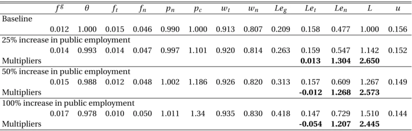
Table2presents the simulated results of the model with a job creation policy scenario that tar-gets increases of 25, 50 and 100% in the level of public employment,Leg. The size of these public

employment increases is consistent with the public sector employment expansions observed in Spanish cities in the period 1980-2001. These scenarios correspond to increases in the public job finding rate,fg, from 0.012 to 0.014, 0.015 and 0.017, respectively.

Increasing public employment in a city implies a higher demand for the non-tradable good.

14_{It is not always obvious whether to classify household expenditure as tradable or non-tradable spending at the}

city level. In general, we consider services to be non-tradable goods.

15_{Imputed rents from the Living Conditions Survey (LCS) look abnormally low in Spain. We take rental values}

from a leading listing website (Fotocasa). In 2012, the average rent was 7.220 euros a month per square meter. The average dwelling in Spain is 90.6m2(2011 Population and Housing Census) which gives us an annual rent of 7,850 euros. If we take the average household income in Spain (26,775 euros according to LCS), we obtain a share of income spent on housing of 0.293.

(16)

Table 1: Calibrated parameter values

Parameters Value Source/Target

Interest rate,r 0.012 Data

Separation rate public sector,sg 0.009 SLFS

Separation rate tradable sector,st 0.015 SLFS

Separation rate non-tradable sector,sn 0.015 SLFS

Matching function elasticity parameter,χ 0.600 (Pissarides and Petrongolo,2001) Matching function scale parameter,mo 0.061 Matching function

Wage public sector,wg 1.000 Normalization

Exogenous productivity tradable sector,At o 1.331 Eurostat &L=1

Agglomeration economies’ elasticity,ζ 0.030 (Combes and Gobillon,2015) Land cost to city size elasticity,η 0.720 (Combes et al.,2012)

Non-tradable good income share,φ 0.600 HBS

Land income share,δ 0.070 LCS, BBVA &Fotocasa

Workers’ bargaining power,β 0.313 Solves23,24,25,30and31 Non-labor income,b 0.315 Solves23,24,25,30and31 Unemployment utility,z 0.308 Solves23,24,25,30and31 Vacancy cost tradable sector,kt 0.944 Solves22

Vacancy cost non-tradable sector,kn 0.415 Solves23,24,25,30and31

Variables

Public employment rate,eg 0.209 2001 Census

Tradable employment rate,et 0.158 2001 Census

Non-tradable employment rate,en 0.477 2001 Census

Unemployment rate,u 0.156 2001 Census Labor market tightness,θ 1.000 Normalization Wage tradable sector,wt 0.913 MCVL

Wage non-tradable sector,wn 0.807 MCVL

Labor force,L 1.000 Normalization Job finding rate public sector,fg 0.012 Solves27

Job finding rate tradable sector, ft 0.015 Solves28

Job finding rate non-tradable sector,fn 0.046 Solves29

Land price,pc 1.000 Solves32

Productivity tradable sector,At 1.331 Eurostat &L=1 & Solves33

(17)

However, expanding public employment with well paid jobs increases local private wages and, thus, employment in the non-tradable sector may either increase or decrease. The simulations indicate that the demand effect clearly dominates the wage effect. Specifically, one public sector job creates between 1.2 and 1.3 jobs in the non-tradable sector. In contrast, an increase in public employees does not raise the demand for locally produced tradable goods. As a result, the effect on tradable employment is smaller and is determined by two opposing forces: higher wages, on the one hand, decrease employment, while agglomeration economies, on the other, increase employment. In this sector, the simulations imply multipliers that are either positive but very small (0.013) or negative (-0.054 to -0.012).

Table 2 also indicates that an increase in the number of public jobs in the city increases the size of its labor force. These effects are substantial. An additional public job increases the city’s labor force by 2.4 to 2.7 workers. A larger city increases the price of land as well as the price of the non-tradable good. This higher cost-of-living (the price indexP) offsets better labor market prospects. The population inflow weakens the link between more jobs and a lower un-employment rate in the city. For instance, increasing public un-employment by 50% only reduces the unemployment rate from 0.156 to 0.149. Similarly, if we focus on employment rates instead of employment levels, the local labor market effects of public employment are not so positive. If we take the scenario of a 50% increase in public employment, the share of workers employed in the private sector actually falls. While the employment rate in the non-tradable sector increases very little (by 0.004), the employment rate in the tradable sector falls by 0.034, which is very simi-lar the increase in the employment rate in the public sector (i.e. 0.038). The same picture occurs if we examine the job finding rates. In the tradable sector, the rate falls from 0.015 to 0.012, while in the non-tradable sector it increases from 0.046 to 0.048. The same pattern is found with the vacancy rate (the sum of the vacancy rates in the tradable and non-tradable sectors) which falls more than the unemployment rate and, as a consequence, labor market tightness actually decreases.

Table 2: Benchmark simulated results with an increase in public employment fg θ ft fn pn pc wt wn Leg Let Len L u

Baseline

0.012 1.000 0.015 0.046 0.990 1.000 0.913 0.807 0.209 0.158 0.477 1.000 0.156 25% increase in public employment

0.014 0.993 0.014 0.047 0.997 1.101 0.920 0.814 0.263 0.159 0.547 1.142 0.152

Multipliers 0.013 1.304 2.650

50% increase in public employment

0.015 0.988 0.012 0.048 1.002 1.186 0.926 0.820 0.313 0.157 0.609 1.267 0.149

Multipliers -0.012 1.268 2.573

100% increase in public employment

0.017 0.978 0.010 0.050 1.011 1.34 0.935 0.830 0.418 0.147 0.729 1.510 0.144

Multipliers -0.054 1.207 2.445

Note: Multipliers are calculated as the employment or labor force change divided by the employment increase in the public sector.

(18)

3.3 Alternative simulations of the model

In this section we present model simulations for two alternative scenarios. First, we consider the model without geographic mobility. Second, we study the relationship between the size of the multipliers and the magnitude of the public sector wage gap.

3.3.1 The model without labor mobility

We consider the model with a fixed city size (L=1), which implies that the productivity in the tradable sector and the price of land are fixed. Since there is no mobility, it is no longer true that

rU =z. In terms of the equations that characterize the equilibrium, we drop equations30,32 and3316. Table3shows the simulated results with an increase in the public job creation rate from 0.012 to 0.020 (a 50 % increase in the level of public employment).

Table 3: Simulated results without labor mobility across cities

fg θ ft fn pn pc wt wn Leg Let Len L u

Baseline

0.012 1.000 0.015 0.046 0.990 1.000 0.913 0.807 0.209 0.158 0.477 1.000 0.156 50% increase in public employment

0.020 0.925 0.006 0.053 1.008 1.000 0.934 0.832 0.314 0.059 0.488 1.000 0.139

Multipliers -0.944 0.105 0.000

Note: Multipliers are calculated as the employment change divided by the employment increase in the public sector.

In stark contrast with the case considered above in which geographic mobility was consid-ered, public employment clearly crowds-out private employment. While one extra job in the public sector destroys about 0.9 jobs in the tradable sector, it only creates 0.1 jobs in the tradable sector. As discussed above, the tradable sector is more negatively affected than the non-tradable sector as an increase in the number of public employees does not increase the demand for locally produced tradable goods. Since one public sector job destroys less than one job in the private sector, unemployment is reduced, falling from 0.156 to 0.139. In this scenario, the link between more public sector jobs and less unemployment is not weakened by the inflow of work-ers but rather by the destruction of private sector jobs. Considering a closed economy brings the results of the simulations much more closely in line with those of the macroeconomics literature analyzing the impact of public employment on (national) labor markets (Burdett(2012),Gomes (2015a),Bradley et al.(2015) andAlgan et al.(2002)).

These simulations show that whether public employment crowds-in or crowds-out private employment depends crucially on the extent to which city size increases following a public em-ployment expansion. In fact, even if workers are mobile, public emem-ployment can not trigger an inflow of workers if land supply is very inelastic, which results in public employment crowding-out private jobs. Indeed, the simulations (not reported here for reasons of space) indicate that

16_{As shown in Appendix}_B_{, the wage equations are obtained without using the condition}_rU

(19)

the elasticity of land price with respect to city size (η), together with the income share spent on land (δ), are the key parameters governing whether (and the extent to which) public employ-ment crowds-in or crowds-out private employemploy-ment.

3.3.2 Size of multipliers and the public wage premium

We simulate two alternative scenarios that differ in the size of the wage gap between the public and the private sectors. In each scenario, we recalibrate the model maintaining the rest of the targets and simulating the effect of an increase in public employment of 50%. First, we reduce the public sector wage gap to 10% while, later, we increase it to 30%. The baseline scenario (Table2, row 2) is reproduced here in the second row for ease of comparison, and it corresponds to a public sector wage gap of 20%. Table4shows the simulated results.

Table 4: Simulation results: Size of multipliers and the public wage premium fg _θ _f

t fn pn pc wt wn Leg Let Len L u

50% increase in public employment & 10% public wage gap

0,016 0,990 0,049 0,012 1,082 1,140 1,007 0,892 0,312 0,137 0,575 1,200 0,146

Multipliers -0.203 0.950 1.938

50% increase in public employment & 20% public wage gap (Table2, second row)

0.015 0.988 0.012 0.048 1.002 1.186 0.926 0.820 0.313 0.157 0.609 1.267 0.149

Multipliers -0.012 1.268 2.573

50% increase in public employment & 30% public wage gap

0,014 0,987 0,048 0,013 0,934 1,218 0,856 0,759 0,315 0,170 0,633 1,315 0,151

Multipliers 0.111 1.470 2.979

Note: Multipliers are calculated as the employment or labor force change divided by the employment increase in the public sector.

The simulations indicate that higher public sector wages increase the positive multiplier ef-fects of public employment. Increasing the public wage gap from 10 to 30% increases the esti-mated employment multipliers from -0.2 to 0.1 in the tradable sector, and from 0.9 to 1.5 in the non-tradable sector. Similarly, the labor force multiplier increases from 1.9 to 3. This result is consistent with the findings reported inMoretti(2010) andMoretti and Thulin(2013). Specifi-cally, they find multipliers from the tradable to the non-tradable sectors that are especially high when the jobs in the tradable sector command high wages. Here, too, the effects of public em-ployment on private emem-ployment are quite sensitive to the public sector wage gap.

4 Reduced-form estimates: Evidence from the late development

of the Spanish public sector: 1980-2001

In this section, using regression analysis, we estimate the city-level effects of public sector job expansions. To that end, we exploit the uneven geography of the substantial increase in pub-lic sector employment that took place in Spain in the period 1980-2001 following the advent

(20)

of democracy. Since we are interested in the long-run effects of public employment (changes between steady states in terms of the model developed above), we examine decadal changes (1980-1990 and 1990-2001) in the employment and population of Spanish cities. This exercise enables us to assess the degree to which the simulated results of the model match carefully esti-mated reduced-form coefficients. This section is organized as follows. After describing the data and variables used in the analysis, we provide a description of the geography of the expansion of public sector jobs. Then, we report Ordinary Least Squares (OLS) estimates before turning to the main instrumental variable analysis that uses a city’s capital status as an instrument for local public sector employment growth.

4.1 Data and variables

We draw primarily on Census data on employment and population. In the case of employment, the data are drawn from Censuses of Establishments carried out in 1980, 1990 and 2001, which contain counts of employees by municipality and by the main economic activity (2-digit level) of the establishment in which the employee works. In the case of population, we use population counts by labor market status from the 1981, 1990 and 2001 Population Censuses. We also have access to some data on employment and population from the 1970 Censuses. We then construct city-wide counts of these variables using the 2008 urban area definitions built by the Ministry of Housing17. We work with a total of 83 cities (urban areas) whose locations and extensions are shown in Figure 1. In 2001, these cities concentrated 67% of the population18. The median city (Ourense) had 126,410 inhabitants in 2001. The size of the two largest cities - Madrid (5,135,225) and Barcelona (4,391,196)- exceeds that of Soria (35,151) and Teruel (33,158) -the smallest two-by a factor of one hundred.

Our public sector definition includes three industries: public administration (which includes the police and military forces), education and health. There are workers in the education and health sectors that are not public employees. Unfortunately, our data does not allow us to distin-guish between private and public employees in these two activities. With this caveat in mind, we include the education and health sectors in our definition of the public sector for two reasons: First, because the majority of these workers are directly employed by governments (in 1999, 67 and 61% of the workers in education and health, respectively19); and, second, because there are many public services in education and health that, being partly financed by the public sector, are provided by private firms. The main instance of this is that of primary and secondary edu-cation where the teachers’ salaries in the majority of privately run schools (so-calledEducación concertada) are paid by regional governments. Similar arrangements also exist in the health

17_{The same definitions are used in}_{De la Roca and Puga}₍₂₀₁₃_).

18_{We do not consider Ceuta and Melilla, the two Spanish enclaves in North Africa.} 19_{These figures have been computed with the first term Labor Force Survey of 1999.}

(21)

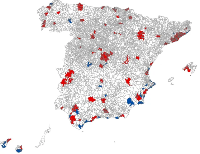
Figure 1: Urban areas (cities) in Spain

Source: Cities (urban areas) in 2008 -Ministerio de la vivienda. Capital cities (52) in red and non-capital cities (31) in blue. The map excludesMenorca(far east) andLa Palma,La GomeraandEl Hierro(far west) as no urban area is found in these islands.

sector.

Total employment is the sum of employees in the public sector (Eg), the tradable sector (Et)

and the non-tradable sector (En)20. We assimilate the tradable sector with the manufacturing

in-dustries, while non-tradable employment contains the workers in private activities that produce goods that can not be traded and includes the construction sector21. Our model also predicts that public sector expansions increase city size. Thus, we also consider (changes in) the city-level (economically) active population, working age population and total population. Since in the model developed above all individuals are active in the labor market, the city size measure used thereLcorresponds more closely to active population.

In the regression analysis, we examine decadal (1980-1990 and 1990-2001) increases in the employment and population measures detailed above relative to the city population in the base

20_{We do not consider agriculture, farming and mining activities as they have been treated differently in different}

Censuses.

21_{Business services are clearly tradable goods. However, the 2-digit industry classification that is available to us}

(22)

year (1980 or 1990). The first two panels of Table5provide summary statistics for employment and population levels in 1980 and 2001 at the city level. The third panel reports summary statis-tics for the outcome variables that we examine below, namely, pooled employment and popula-tion decadal changes (1980-1990 and 1990-2001) relative to the populapopula-tion level at the beginning of the decade.

Table 5: Employment and population in Spanish cities (1980-2001): Summary statistics

Variable Mean Median SD Min Max

Employment and population levels in 1980 (N=83)

Tradable employment 21,127 5,577 61,225 113 474,588 Non-tradable employment 30,026 10,625 75,550 1,551 513,539 Total employment 64,353 18,914 163,557 2,032 1,067,467 Active population 82,000 23,789 208,017 2,526 1,367,068 Working age population 180,138 52,284 428,575 10,672 2,812,315 Total population 296,136 96,763 689,109 18,022 4,546,343 Public employment 13,200 5,495 30,638 368 243,589 Employment and population levels in 2001 (N=83)

Tradable employment 22,523 6,218 62,847 993 487,367 Non-tradable employment 67,688 23,003 172,171 5,397 1,252,375 Total employment 119,700 43,641 294,959 10,447 2,033,004 Active population 141,829 52,138 340,127 13,247 2,357,121 Working age population 228,056 87,123 520,014 19,828 3,609,102 Total population 330,320 126,410 747,146 31,158 5,135,225 Public employment 29,489 12,459 64,742 1,872 488,260 Employment and population decadal changes relative to the city’s

population in the base year (1980-1990 & 1990-2001 pooled changes, N=166) Tradable employment 0.005 0.005 0.019 -0.052 0.115 Non-tradable employment 0.061 0.052 0.041 -0.067 0.264 Total employment 0.095 0.089 0.058 -0.137 0.308 Active population 0.109 0.103 0.060 -0.119 0.356 Working age population 0.109 0.090 0.091 -0.029 0.584 Population 0.105 0.078 0.160 -0.088 0.959 Public employment 0.029 0.028 0.019 -0.031 0.093 Control variables: Pooled observations for 1980 and 1990 (N=166)

Unemployment rate 0.181 0.170 0.061 0.042 0.406 Share of college graduates 0.080 0.079 0.032 0.024 0.170

Coast 0.446 0.000 0.499 0 1

Coast north 0.084 0.000 0.279 0 1

Share of vacation-homes in 1991 18.684 11.603 16.252 3.830 77.826 Total population in 1970 240,644 75,857 566,044 12,776 3,630,338 Note: Variables as defined in the main text.

Starting with total population, the city average increased by 11.5% between 1980 and 2001. Since the sample is fixed over time (N=83), 11.5 is also the growth rate of the entire urban popu-lation in Spain. This figure exceeds 8.6%, the popupopu-lation growth experienced by Spain as a whole

(23)

during this period, and indicates that the share of the population living in urban areas increased between 1980 and 2001. This higher growth experienced by cities is explained mostly by in-traregional migrations from rural areas to cities (Bover and Arellano(2001) andJofre-Monseny (2014)). Note that the average population growth rate over one decade (third panel) is 10.5%, which reveals that in Spain, small cities have grown more than large cities. In fact, mean rever-sion in population growth is a prevalent feature of our city-level data and one that needs to be taken into account in the regression analysis. The economically active population has grown far more (73%) in Spanish cities during this period as women entered the labor force en masse22. Similarly, (urban) employment increased by 86% between 1980 and 2001. This increase was not uniform across economic sectors as the economy experienced a process of tertiarization with employment in the tradable sector growing by only 6.6% between 1980 and 2001.

4.2 The geography of public sector employment expansion

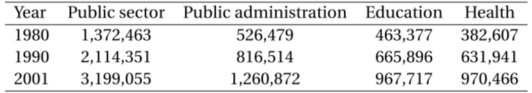
In Spain, the public sector developed at a surprisingly late date. Development started with the advent of democracy following Franco’s death in 1975 and the introduction of the new constitu-tion in 1978. While in 1980, the tax revenue to GDP ratio was only 22.6%, by 2001 this ratio had reached 33.9%23. This growth in the relative size of the public sector, combined with vigorous economic growth (the average annual real GDP growth rate between 1980 and 2001 was 2.95%) resulted in very large increases in public sector jobs. Table6shows the number of jobs in public administration, education and health in 1980, 1990 and 2001.

Table 6: Public sector jobs in Spain (1980-2001)

Year Public sector Public administration Education Health 1980 1,372,463 526,479 463,377 382,607 1990 2,114,351 816,514 665,896 631,941 2001 3,199,055 1,260,872 967,717 970,466 Source: Nationwide employment counts.

Between 1980 and 2001, there were job increases of 139, 109 and 154% in public adminis-tration, education and health, respectively. Taking the three sectors together, the increase in the number of public sector jobs during this period amounts to 133%, growing from 1.4 million in 1980 to almost 3.2 million jobs in 2001. For the three sectors making up the public sector as defined herein, public administration increased from 0.526 to 1.261 million jobs, the educa-tion sector rose from 0.463 to 0.967 million while employment in the health sector went from 0.382 to 0.970 million. In the urban areas studied here, the increase in public sector jobs was

22_{According to the 1981 and 2001 Censuses, between these two years the participation rate of females aged 25-64}

increased from 21 to 58%

(24)

slightly lower than that recorded in Spain as a whole (123 versus 133%). This, coupled with the higher population growth of the urban areas, implies that public sector employment has grown disproportionately more in the non-urban areas of Spain.

Across cities, public sector jobs are also unevenly distributed. The size of the public sector is determined by and large by its administrative status. In Spain, there are provincial and regional capitals. Provinces (and the associated capitals) were established in 1833 by Javier de Burgos and constituted the main territorial division of the country until the advent of democracy. Al-though the provinces were not suppressed, 17 regions (Comunidades Autónomas) were built as aggregations of one or more provinces in 1981. Twenty years later, Spain was a decentralized country in which the spending of theComunidades Autónomasamounted to roughly 46% of to-tal government spending24. A similar picture is obtained if we look at the distribution of public employees across tiers of government. In 2001, regional governments employed 45% of public employees whereas the central government and local governments employed the remaining 34 and 21%25.

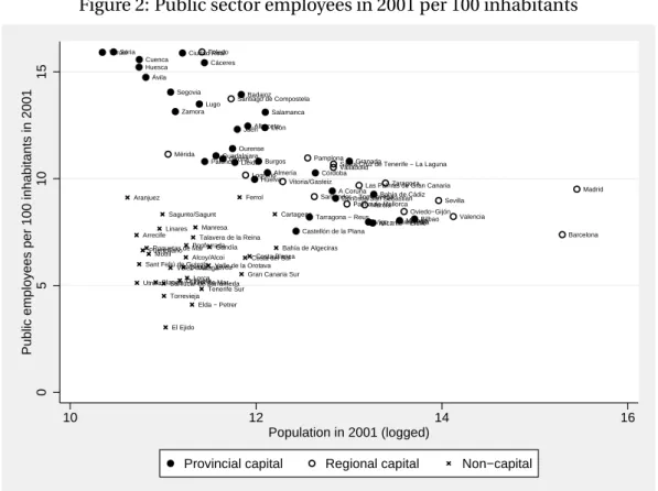
Figure 2plots the presence of public employees in cities, distinguishing between regional and provincial capitals, and non-capital cities. With two exceptions (Santiago de Compostela and Mérida), the cities hosting regional governments are also provincial capitals26. Non-capital cities, such as El Ejido, Elda-Petrer and Torrevieja, have the lowest presence of public employees in 2001 with less than 5 employees per 100 inhabitants. At the other end of the scale, provincial capitals, such as Soria, Teruel, Ciudad-Real and Toledo, have more than 15 public employees per 100 inhabitants. More generally, this figure corroborates that being a capital is associated with public employees, and the difference is especially large for small cities. Holding population size constant, the presence of public employment is similar in provincial and regional capitals. This suggests that the process of regional decentralization that took place in Spain between 1981 and 2001 was not accompanied by a significant shift in public employment from provincial to regional capitals. On the contrary, pre-democratic provincial capitals kept theirstatus quoin terms of public employment. On the one hand, provincial institutions (Diputacionesbeing the most prominent example) persisted into democratic Spain. On the other hand, provincial cap-itals managed to attract regional government public jobs. In the light of this, we only consider two types of city: capitals (regardless of their being provincial or regional) and non-capitals. There are 52 capital cities (50 provincial capitals in addition to Santiago de Compostela and Mérida) and 31 non-capital cities. Figure1 shows the capital cities (in red) and non-capital cities (in blue) within Spain.

24_{Excluding social security spending. See}_{Carrión-i Silvestre et al.}₍₂₀₀₈_{) for a detailed explanation of the}

decen-tralization process.

25_{Registro Central de Personal, Ministerio de Hacienda y de Administraciones Públicas.}

26_{These two cities are historically important. Mérida was the capital of the Roman Lusitania province and}

San-tiago is the destination of a major Catholic pilgrimage route. Moreover, these are the third cities in two bicephalic regions: Galicia (La Coruña and Vigo) and Extremadura (Cáceres and Badajoz).

(25)

Figure 2: Public sector employees in 2001 per 100 inhabitants MálagaBilbao Alicante − Elche Bahía de Cádiz Vigo − Pontevedra Granada A Coruña Donostia/San Sebastián Tarragona − Reus Córdoba Castellón de la Plana Almería León Salamanca Burgos Huelva Albacete Lleida Badajoz Girona Guadalajara Jaén Ourense Cáceres Palencia Lugo Ciudad Real Segovia Zamora Ávila Cuenca Huesca Soria Teruel Madrid Barcelona Valencia Sevilla Oviedo−Gijón Zaragoza Murcia

Las Palmas de Gran Canaria

Palma de Mallorca Santa Cruz de Tenerife − La Laguna Valladolid Pamplona Santander − Torrelavega Vitoria/Gasteiz Logroño Santiago de Compostela Toledo Mérida Bahía de Algeciras Costa Blanca Cartagena

Costa del Sol

Gran Canaria Sur

Tenerife Sur Ferrol

Gandía

Torrevieja

Denia − JáveaValle de la Orotava Orihuela Manresa Talavera de la Reina Lorca Elda − Petrer Ponferrada

Blanes − Lloret de Mar Vélez−Málaga Alcoy/Alcoi El Ejido Roquetas de Mar Sagunto/Sagunt Sanlúcar de Barrameda Linares

Sant Feliú de Guixols Motril Arrecife Aranjuez Puertollano Utrera 0 5 10 15

Public employees per 100 inhabitants in 2001

10 12 14 16

Population in 2001 (logged)

Provincial capital Regional capital Non−capital

Source: Census and own elaboration.

Figure3plots the (per capita) increase in public sector employment between 1980 and 2001 in the capital and non-capital cities. It shows that when public sector employment grew after the advent of democracy, growth was more pronounced in the capital cities, the differences being especially notable in small cities. The first row in Table7quantifies the (raw) over-representation of public employment in the capital cities. While the non-capital cities had 6.3 public sector workers per 100 inhabitants in 2001, the corresponding figure for the capital cities was 11.1. Al-though the difference is smaller in magnitude, per capita public sector workers also increased more in the capital cities between 1981 and 2001. The increase was 3.6 in non-capital cities vs. 5.1 in capital cities. Rows 1 to 4 in Table7show that the over-representation of public em-ployment in capital cities, both in 2001 levels as well as in the changes between 1980 and 2001, occurred in public administration but also in the education and health sectors, as institutions like universities and hospitals also tend to concentrate in capital cities.

We now turn to a more systematic analysis of the city-level determinants of the public sector employment expansion in the period 1980-2001. Specifically, we run regressions of the following type:

Eg,t+10−Eg,t

Popt =αt+β·

C api t al+δz+²t (34)

(26)

Figure 3: Public sector job increase between 1980 and 2001 per 100 inhabitants Madrid Barcelona Valencia Sevilla Málaga Bilbao Oviedo−Gijón Zaragoza

Alicante − ElcheBahía de Cádiz Murcia

Vigo − Pontevedra Las Palmas de Gran Canaria

Palma de Mallorca Granada

Santa Cruz de Tenerife − La Laguna A Coruña Valladolid Donostia/San Sebastián Tarragona − Reus Pamplona Córdoba Santander − Torrelavega Castellón de la Plana Vitoria/Gasteiz Almería León Salamanca Burgos Huelva Logroño Albacete Lleida Badajoz Girona Guadalajara Jaén Santiago de Compostela Ourense Toledo Cáceres Palencia Lugo Ciudad Real Segovia Zamora Mérida Ávila Cuenca Huesca Soria Teruel Bahía de Algeciras Costa Blanca Cartagena Costa del SolGran Canaria Sur

Tenerife Sur Ferrol Gandía Torrevieja Denia − Jávea Valle de la Orotava Orihuela Manresa Talavera de la Reina

Lorca Elda − Petrer Ponferrada

Blanes − Lloret de Mar Vélez−Málaga Alcoy/Alcoi El Ejido Roquetas de Mar Sagunto/Sagunt Sanlúcar de Barrameda Linares Sant Feliú de Guixols

Motril Arrecife Aranjuez Puertollano Utrera 0 2 4 6 8 10

Public sector jobs increase (80−01) per 100 inhabitans

10 11 12 13 14 15

Population in 1980 (logged)

Capitals Non−capitals

Source: Census and own elaboration.

Table 7: Public sector jobs in capital versus non-capital cities (per 100 inhabitants)

2001 1980-2001

Capital Non-capital Capital Non-capital Public sector 11.120 6.320 5.140 3.550 Public administration 4.530 2.390 2.060 1.460 Education 3.170 1.950 1.510 0.850

(27)

1990-2001) relative to the population level in the base year (1980 or 1990)27. In turn,αt is a set

of time dummies whileC api t al is an indicator variable for capital cities. Finally, z contains some control variables that we consider in some of the specifications. The results are reported in Table8.

The first column shows the results with no other control variables than time dummies. These estimates indicate that, in the period 1980-2001, being a capital implied an additional 0.7 public workers each decade for every 100 inhabitants in the city in the base year. In the second column, we also consider population growth as a control variable despite its endogenous nature (public sector jobs might increase population as the model developed above predicts). When doing so, the capital effect increases, implying that being a capital is associated with 1.1 extra public jobs for every 100 inhabitants each decade. To assess the relative magnitude of this effect, note that the population growth coefficient (0.036) indicates that an increase of 100 residents is associated with an increase of 3.6 public sector workers. As explained above, there is ample evidence from different countries indicating public employment is used to offset local labor demand shocks. To test if this has also been the case in our application, in the last specification (column 3), we include aBartik(1991) shift-share variable that captures demand driven private employment changes in city: Ep,t+10−Ep,t Popt = P h µ Eh,t ENe h,t ENe h,t+10−Eh,t ¶ Popt , (35)

whereEp stands for private employment (the sum of tradable and non-tradable workers),h

indexes the (2-digit) industries within the private sector whileNe denotes national employment

levels. The predicted employment change in equation35captures the component of the 1980-1990 and 1980-1990-2001 local employment shock explained by the city’s industry mix in the base year (1980 or 1990) interacted with the decadal (1980-1990 or 1990-2001) fate of industries at the national level. The results indicate that for each job lost as a result of a demand shock in a city, the public sector has created 0.194 jobs in the public sector in that city. This provides direct evidence that public employment has been used as a prominent policy instrument to offset local economic shocks. Note that these policy responses are important since they will bias downwards the OLS estimates in the regressions (which we turn to next) that estimate the effect of public employment on local private employment. As for the capital variable, the results of this last specification are slightly higher, implying that capital cities gained 1.6 additional public sector jobs per decade for every 100 inhabitants in the period 1980-2001.

27_{This variable will become the main explanatory variable in the next section when we turn to the multiplier}

(28)

Table 8: The determinants of public sector job increases (1) (2) (3) Capital 0.007*** 0.011*** 0.016*** (0.002) (0.002) (0.003) Population growth 0.036*** 0.042*** (0.007) (0.008) Ep,t+10−Ep,t Popt -0.194*** (0.060) R-squared 0.041 0.119 0.165 Observations 166 166 166 Notes: 1) 1980-1990 and 1990-2001 pooled observations 2) Robust standard errors clustered at the city-level in parentheses. 3) *** de-notes statistical significance at the 1% level. 4) Population growth is the contemporaneous decadal population growth rate. 5) The last ex-planatory variable, the private job changes’ predictor, as defined in equation35.

4.3 Public employment multipliers: OLS estimates

We now turn to the estimation of public sector employment multipliers. Specifically, we esti-mate the impact of (decadal) changes in public employment on contemporaneous changes in measures of employment and population. All employment and population changes are divided by the city’s population level at the beginning of the decade. We run variants of the following specification. Yt+10−Yt Popt =µt+γ Eg,t+10−Eg,t Popt +ηxt+ζt, (36)

whereY stands for tradable, non-tradable and total employment, and active, working age, and total population. In addition to the change in public employment (Eg), the specification

includes time dummies (µt), a vector containing control variables (xt) and the error term (ζt).

The results are reported in Table9where each row shows the effect of a public sector job increase on a different outcome. The first column shows the results of specifications that only include the time dummies as controls. In the second column, we also include the unemployment rate and the share of college graduates measured at the beginning of the decade. Some of the cities in our sample are fast-growing coastal cities associated with tourism, such as Torrevieja, Costa del Sol or Tenerife Sur. Thus, in the third column we also include the share of vacation homes in 1991 as well as two coastal indicators: one for the North Atlantic coast (Mar Cantábrico) with less tourism and one for the coasts of the Mediterranean, the Andalusian Atlantic and the Canaries coasts. Finally, as commented previously, when describing the summary statistics in Table5, there is mean reversion in population growth. Hence, in column 4, we include a second order

(29)

polynomial of the (logged) population level in 1970. The summary statistics for these controls are provided in the bottom panel of Table5.

Table 9: Public employment multipliers: OLS estimates

Outcomes: 1 2 3 4 a)Tradable employment 0.087 0.116* 0.101 0.102 (0.073) (0.060) (0.064) (0.064) b) Non-tradable employment 0.545*** 0.649*** 0.602*** 0.614*** (0.156) (0.145) (0.134) (0.133) c) Total employment 1.632*** 1.765*** 1.703*** 1.716*** (0.183) (0.164) (0.160) (0.160) d) Active population 1.780*** 1.940*** 1.853*** 1.862*** (0.211) (0.185) (0.168) (0.169) e) Working age population 0.938** 1.117*** 0.865*** 0.865***

(0.438) (0.421) (0.334) (0.295) f ) Population 1.679*** 1.875*** 1.447*** 1.458***

(0.573) (0.576) (0.456) (0.452)

Unemployment rate N Y Y Y

Share of college graduates N Y Y Y

Coastal dummies N N Y Y

Share of vacation-homes in 1991 N N Y Y Logged pop in 1970 (2nd order pol.) N N N Y

N 166 166 166 166 <